VALEUR AJOUTÉE DANS
LE MODÈLE REGIONAL CANADIEN DU CLIMAT: COMPARAISON DE LA PRÉCIPITATION
AUX ÉCHELLES DU MODÈLE GLOBAL CANADIEN DU CLIMAT
MÉMOIRE
PRÉSENTÉ COMME EXIGENCE PARTIELLE DE LA MAÎTRISE EN SCIENCES DE L'ATMOSPHÈRE
PAR
ALEJANDRO DI LUCA
UNIVERSITÉ DU QUÉBEC À MONTRÉAL
ADDED VALUE IN THE CANADIAN REGIONAL CLIMATE MODEL: COMPARlSON OF PRECIPITATION
AT THE SCALES OF THE CANADIAN GLOBAL CLIMATE MODEL
THESIS
PRESENTED IN PARTIAL FULLFILMENT
OF THE REQUlREMENTS FOR THE MASTER'S DEGREE IN ATMOSPHERIC SCIENCES
BY
ALEJANDRO DI LUCA
Avertissement
La diffusion de ce mémoire se fait dans le respect des droits de son auteur, qui a signé le formulaire Autorisation de reproduire et de diffuser un travail de recherche de cycles supérieurs (SDU-522 - Rév.ü1-2üü6). Cette autorisation stipule que «conformément à l'article 11 du Règlement no 8 des études de cycles supérieurs, [l'auteur] concède à l'Université du Québec à Montréal une licence non exclusive d'utilisation et de publication de la totalité ou d'une partie importante de [son] travail de recherche pour des fins pédagogiques et non commerciales. Plus précisément, [l'auteur] autorise l'Université du Québec à Montréal à reproduire, diffuser, prêter, distribuer ou vendre des copies de [son] travail de recherche à des fins non commerciales sur quelque support que ce soit, y compris l'Internet. Cette licence et cette autorisation n'entraînent pas une renonciation de [la] part [de l'auteur] à [ses] droits moraux ni à [ses] droits de propriété intellectuelle. Sauf entente contraire, [l'auteur] conserve la liberté de diffuser et de commercialiser ou non ce travail dont [il] possède un exemplaire.»
REMERCIEMENTS·
À mon directeur, René Laprise, pour ses précieuses contributions à ce travail et pour son encouragement constant tout au long de la maîtrise.
À mon codirecteur, Ramon de Elîa, avec qui il est si agréable de travailler et qui m'a poussé à réfléchir au-delà des questions scientifiques. Ainsi que par ses généreux conseils qui m'ont aidé énormément au cours des dernières deux années.
À Ross Brown pour les intéressantes discussions au sujet des observations de précipitation. À Georges, Abderrahim et Mourad pour leur inestimable aide technique. Aux membres de l'équipe de simulation climatique d'Ouranos, en particulier à Anne, Michel et Dominique qui, entre autres choses, m'ont aidé avec les données du MRCC.
À tous les collègues et amis de l'UQAM et d'Ouranos, qui sont toujours prêts à donner un coup de main quand j'en ai eu besoin et qui ont égayé quelques soirées à l'extérieur du travail.
Au centre ESCER pour Je soutien financier et au Consortium Ouranos pour ['espace physique où j'ai pu accomplir ma recherche.
À la famille et les amis, qui même à distance, sont toujours le support moral et la plus grande source d'inspiration.
Finalement, à mes colocataires: Anso, Caro, Guigui et Nico, qui sont en grande partie responsables de ces deux dernières années très heureuses.
LISTE DES ABRÉVIATIONS, SIGLES ET ACRONyMES xiii
LISTE DES SyMBOLES xv
RÉSUMÉ xvii
INTRODUCTION 1
CHAPITRE 1 5
VALEUR AJOUTÉE DANS LE MRCC : COMPARAISON DE LA PRÉCIPITATION
AUX ÉCHELLES DU MGC 5
Abstract 9
1. Introduction Il
2. Issues in the evaluation of added value 15
2.1 Availability of observed data 15
2.2 Point observations vs. model-simulated precipitation 16
2.3 Effective resolution in climate models 17
2.4 Resolved spatial scales: RCM vs GCM 18
3. Data 21
3.1 Observed data: meteorological stations 21
3.2 Coupled Global Climate Model: CG CM 3.1 22
3.3 Regional Climate Model: CRCM 4.2.0 23
4. Methodology 25
4.1. Regions and period of study 25
4.2. Temporal and spatial scales of analysis 27
4.3. Statistical analysis tools 28
4.3.1. Monthly mean values 28
4.3.2. Estimation of precipitation intensity distributions 29
4.3.3. Analysis of dry days 31
4.3 A.Analysis of heavier precipitation rate events 31
5. Results 33
Vlll
5.1.1. The case with one CG CM grid point... 33
5.1.2. The case with four CGCM grid points 34
5.2. Intensity frequency distributions of daily precipitation rate 36
5.2.1 The case with one CGCM grid point.. 36
5.2.2 The case with four CGCM grid points 38
5.3 Heavier precipitation rates 38
6: Summary and Discussion 41
Appendix A: Precision of observed data 45
Appendix B: Construction of histograms and error sampling 49
References 53
FIGURES 59
TABLEAUX 83
CONCLUSION 89
Fig. 1 Spatial scales resolved by a GCM (full blue arrow) and a RCM (full red arrow) with grid spacing of 400 km and 50 km respectively. Aiso indicated is the interval ofwavelengths only resolved by the GCM (blue dotted arrow) and by the RCM (red dotted arrow). The black dashed square designates the spatial scales that will be considered in this study (see
explanations in text) 60
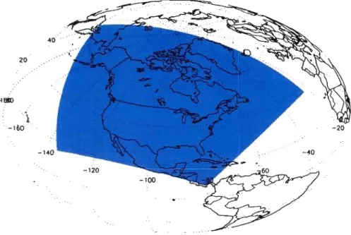
Fig. 2 Computational domain used in the CRCM (201 x 193 grid points) for the two
simulations analyzed 61
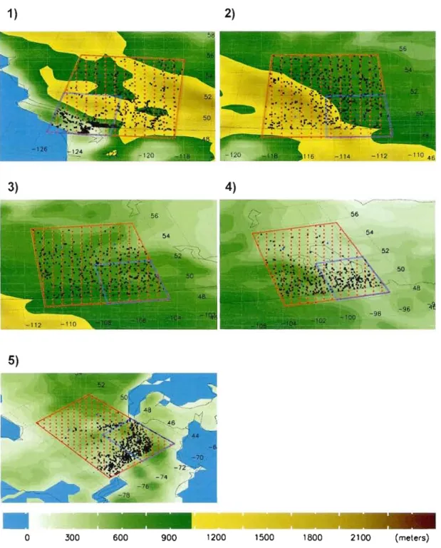
Fig. 4 Weather stations (black points), CRCM grid points (red points) and CGCM grid points (blue points) for regions indicated in Fig. 1: (1) BC, (2) ALTA, (3) SAS, (4) MAN and (5) QC. As in Fig. l, the blue boxes denote those regions including one CGCM grid point and the red ones those regions that include four grid points. The topography field as represented
in the CRCM is shown in color filled contours 63
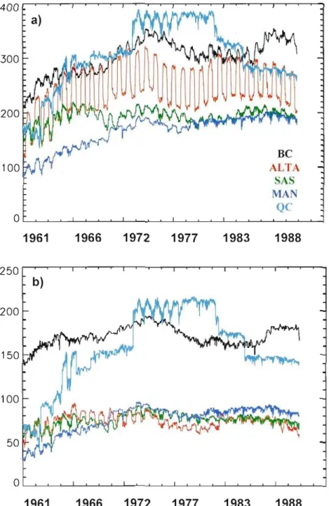
Fig. 5 Number of stations available in each region as a function of days for the period 1961 1990. Each region is indicated with a color. Fig. (a) shows regions including four CGCM grid
points and (b) those regions including only one CG CM grid point. 64
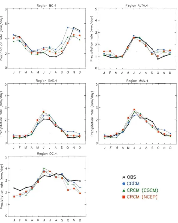
Fig. 6 Observed and simulated monthly mean precipitation rates (mm/day) for ail regions
including one-CGCM grid point... 65
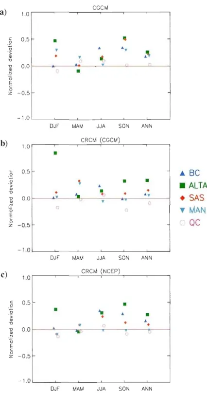
Fig. 7 Deviations between simulated and observed seasonal mean precipitation rate, normalized by observed values, for (a) CGCM, (b) CRCM when driven by the CGCM and (c) CRCM when driven by the NCEPINCAR reanalysis. Different symbols represent each of
the five regions analyzed 66
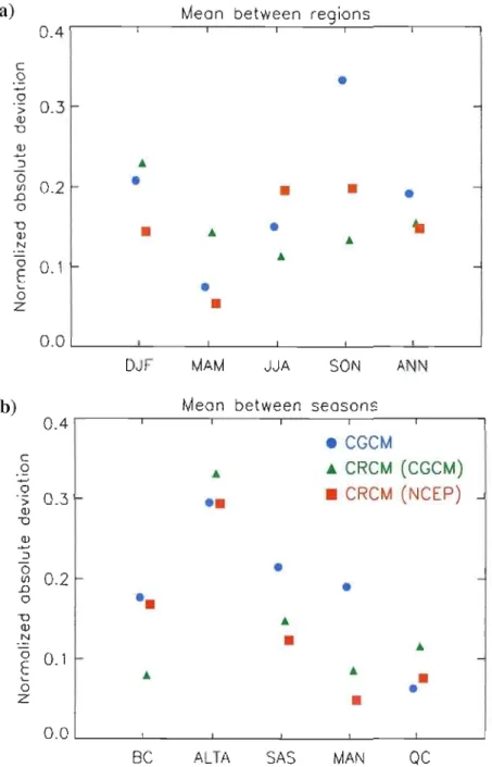
Fig. 8 Absolute deviations between simulated and observed seasonal mean precipitation rate, normalized by observed values, for (a) averaging between regions and (b) mean annual
precipitation rate. Different symbols represent each of the five regions analyzed 67
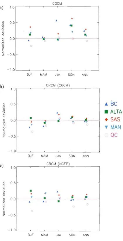
Fig. 9 As in Fig. 6 but for regions including four CGCM grid points 68
Fig. 10 As in Fig. 7 but for regions including four CGCM grid points 69
Fig. II As in Fig. 8 but for regions including four CGCM grid points 70
Fig. 12 Intensity frequency distributions of precipitation rate in DJF for the five regions studied. Observed data is in black, CG CM data in blue, the CRCM when driven by CGCM in green and when driven with NCEPINCAR reanalysis in red. Only frequencies greater than
0,1 % are shown 71
x
Fig. 14 S score (Perkins et al., 2007) calculated between the simulated and observed distribution as a function ofregions for a) DJF, b) MAM, c) JJA and d) SON. Symbols
denote the model used to produce data 73
Fig. 15 Ratio between observed and simulated dry days as a function of regions for a) DJF, b)
MAM, c) JJA and d) SON. Symbols denote the model used to produce data 74
Fig. 16 As in figure 14 but for regions including four CG CM grid points 75
Fig. 17 As in Fig. 15 but for regions including four CG CM grid points 76
Fig. 18 Observed and simulated 95 % percentile calcuJated as a function of region for a) DJF, b) MAM, c) JJA and d) SON. Symbols denote the model used to produce data 77
Fig. 19 As in Fig. 18 but for regions including four CGCM grid points 78
Fig. 20 Normalized precipitation distribution for the full European domain using ail annual data over land only. Symbols denote the model used to produce data (Reproduced from
Christensen et al. 2008) 79
Fig. A.I Observed intensity frequency distributions calculated on the basis of four different bin sizes (only intensities less than 5 mm/day are shown). Regions are indicated with blue
!ines in Fig. l, corresponding to the size of one CGCM grid-box 80
Fig. A.2 Percent frequency distribution of daily precipitation of at least 0.01 in. for the period 1971- 2000 at COOP stations: (a) Bishop, CA (040822), mean an nuaI precipitation of 4. 9 in. (125 mm); and (b) Quillayute, WA (456858), mean annual precipitation of 101.9 in. (2587 mm). Neither station exhibits appreciable observer bias. Solid curve is the fitted gamma function. (Reproduced from Daly et al. (2007) © 2007 American Meteorological Society).... 81
Table 1. Simulations used in the study. Column 1 is the acronym of each simulation used in the text. Column 2 is the name of the model and its source. Column 3 denotes the type of model, the horizontal grid spacingltriangular truncation and the number of vertical levels and column 4 indicates the data used to drive the regional model in each simulation. Finally,
column 5 gives the period of analysis of simulations 84
Table 2. Name, sizes (degrees2) and boundaries in latitude and longitude for the regions
examined in the study. The name of the region is composed by the abbreviated name of the province where it belongs and a digit that refers to the number of CG CM grid points within
the region , 85
Table 3. Number of grid points of each model and number of weather stations within each region for the period 1971-1990. In the case of observed data, the minimum and mean value
of stations are indicated 86
Table 4. Inter-region mean S score (Perkins et al., 2007) calculated between the simulated and observed distribution for each season and for each simulation. Results are presented for both sizes ofregions. Minimum and maximum values in each simulation are denoting in blue
and red respectively 87
Table AI Mean and maximum number ofstations in each region including one CG CM grid point during the period 1971-1990. Aiso presented are, the total number of data and the equivalent number of years of a daily time series built assuming that ail data are from the
AGCM ALTA AOGCM ANSD BBE BC CFL CGCM CRCM DO DJF GCM IPCC JJA LAM LBC MAM MAN MCG MCCG MCGC MINK MRC MRCC NARCAAP NCEP NCAR NSD
LISTE DES ABRÉVIATIONS, SIGLES ET ACRONYMES
Atmospheric genera! circulation mode! Alberta (province of Canada)
Atmosphere-ocean general circulation mode! Absolute normalized seasonal deviation Big Brother Experiment
British Columbia (province of Canada) Conditions aux frontières latérales
version 3 of the Canadian centre for climate modelling and analysis coupled global climate model
Canadian regional climate model Dry days
December-January-February General circulation model
Intergovernmental panel of climate change June-July-August
Limited area model
Lateral boundary conditions March-April-May
Manitoba (province of Canada) Modèle de circulation générale Modèle couplé de circulation générale Modèle de circulation générale canadien Région de Missouri, Iowa, Nebraska et Kansas Modèle régional du climat
Modèle régional Canadien du climat
North American Regional Climate Change Assessment Program National Center for Environmental Prediction
National Centers for Atmospheric Research Normalized seasonal deviation
PR PRUDENCE QC RCM SAS SON UK WD Precipitation rate
Prediction of Regional Scenarios and Uncertanties for Defining European Climate Change Risks and Effects
Quebec (province of Canada) Regional climate model
Saskatchewan (province of Canada) September-October-November United Kingdom
B
f
Gs H j K m mod obsPO
r sLISTE DES SYMBOLES
distribution binomiale fonction histogramme
échelles spatiales résolues seulement par le MCG numéro de classifications dans l'histogramme linéaire indice des stations ou des points de grille
indice des jours
numéro de classifications dans l'histogramme logarithmique indice des mois
données simulées données observées probabilité de ... indice des régions
division entre les jours secs simulés et observés échelles spatiales résolues seulement par le MRC indice des saisons
mesure statistique définie par Perkins et al. (2007) indice des années
taille de la classification (mm/jour)
taille de la classification de l'histogramme logarithmique (mm/jour) intervalle de la grille du MCG (km)
(MRC) constituent une des principales sources de ce type de données puisque les modèles de circulation générale (MCG) ne fonctionnent toujours pas à une résolution suffisante pour répondre à ces besoins.
Une fois que les MRC sont devenus des outils capables de générer des simulations physiquement réalistes, un effort important a été fait pour évaluer leur capacité de mise à l'échelle, en se concentrant principalement sur des variables moyennées temporellement. Cet effort ne s'est pas traduit par des améliorations sans équivoque par rapport aux simulations
produites par les MCG.
L'objectif principal de cette étude est d'examiner ('existence de la valeur ajoutée dans les simulations du modèle régional Canadien du climat (MRCC) par rapport à celles du modèle de circulation général canadien (MCGC) utilisé comme pilote. Dans cette première étape, il a été nécessaire d'analyser les échelles temporelles et spatiales communes aux deux modèles, le MRCC et le MCGC. Une comparaison est effectuée en ramenant les données à haute résolution des stations météorologiques et du MRCC à la résolution du MCGC.
L'évaluation se base sur la comparaison des histogrammes d'intensités de précipitation et des 9Se centiles des distributions afin de caractériser les événements extrêmes. On estime le degré de chevauchement entre les distributions simulées et observées en utilisant la mesure S définie par Perkins et al. (2007). Cette dernière reflète principalement le comportement des intensités faibles et modérées.
Les résultats montrent que les statistiques quotidiennes des précipitations simulées par le MGCC et le MRCC sont généralement très similaires. En comparant les résultats des deux modèles, il n'existe aucune preuve de j'existence de la valeur ajoutée. En outre, pendant l'été, les données simulées par le modèle MCGC sont plus proches des observations que celles générées par le MRCC. Cette amélioration provient d'une meilleure simulation de la fréquence des jours secs. Pour les événements quotidiens les plus intenses, le MCGC produit aussi des résultats plus proches des valeurs observées que le MRCC. Ce dernier montre une sous-estimation constante de la fréquence d'occurrence des événements intenses. C'est aussi le cas dans les régions caractérisées par d'importants forçages de surface, où la différence entre les topographies des deux modèles pourrait avoir un impact.
circulation générale (MCCG). Ces modèles sont dérivés des lois physiques fondamentales et incluent, entre autres, des composants dynamiques décrivant des processus atmosphériques, océaniques, de la surface terrestre, ainsi que de la glace de mer. La dynamique est soumise à des approximations appropriées pour la grande échelle du système climatique (par exemple, l'approximation hydrostatique dans la composante atmosphérique) et la discrétisation des équations provoque une approximation supplémentaire. La multitude et la complexité des processus à résoudre, la longueur nécessaire des simulations pour l'étude du climat, ainsi que la nécessité d'effectuer des ensembles de simulations comprenant plusieurs membres afin d'obtenir des estimations statistiquement robustes imposent des contraintes de temps de calcul qui limitent l'intervalle de la grille sur laquelle les équations sont discrétisées. Présentement, les distances horizontales des grilles atmosphériques varient entre 125 et 400 km (Randall et al., 2007), et elles sont insuffisantes pour reproduire la structure à petite échelle des variables climatiques. Par conséquent, des paramétrages doivent êtres utilisés pour représenter les procédés physiques non résolus. Ainsi, la confiance envers les modèles climatiques pour fournir des estimations quantitatives crédibles du climat est limitée aux échelles continentales et plus grandes (Randall et al., 2007).
Dans ce contexte, une alternative pour obtenir des projections climatiques régionales futures est j'utilisation des modèles régionaux du climat (MRC) à haute résolution, en utilisant des conditions aux frontières latérales (CFL) des MCG à plus basse résolution (Dickinson et al., 1989; Giorgi et Bates, 1989; Laprise, 2006).
La plus haute résolution horizontale des MRC implique deux grands avantages potentiels par rapport aux MCG : une discrétisation plus précise des équations qui permet une plus large gamme d'échelles spatiales explicitement résolues et, peut-être plus importante encore, une amélioration de la représentation des forçages de surface comme la topographie, les contrastes terre - mer, etc.
2
L'impact de l'augmentation de la résolution horizontale a été le sujet de plusieurs études dans les MCG (Boer et Lazare, 1988; Boville, 1991; Boyle, 1993) et dans les MRC (Marinucci et Giorgi, 1996; Castro et al., 2005; Xue et al., 2007), généralement en utilisant des résultats du même modèle mais pour différentes résolutions. Ces études montrent que les simulations à plus haute résolution ne produisent pas nécessairement des résultats plus proches des valeurs observées, mais que les performances dépendent fortement du comportement des paramétrages. En d'autres termes, l'augmentation de la résolution horizontale peut aggraver le comportement des paramétrages des processus de sous échelles et donc, nécessiter de faire appel à des nouveaux paramétrages ou à modifier ceux qui existent déjà. Par exemple, Marinucci et Giorgi (1996) ont étudié des données de précipitation simulés par un MRC à haute résolution et ont constaté que «the effects of physical forcings (e.g., a better representation of topography and coastlines) may be masked by the direct sensitivity of the model parameterizations to resolution itself, at least in the continental scale».
Les avantages provenant de l'utilisation de plus haute résolution des MRC sont influencés non seulement par la sensibilité des paramétrages à la résolution elle-même, mais aussi par la fiabilité technique de mise à l'échelle dynamique. Ici, la fiabilité de la mise à l'échelle dynamique est définie de manière similaire au second principe de Laprise et al. (2007) : la petite échelle générée par le MRC possèdes des amplitudes et statistiques climatiques qui seraient présents dans les données de pilotage si elles n'étaient pas limitées par la résolution. Cette affirmation a été étudiée en isolant les erreurs de la technique de pilotage sans prendre en compte ceux qui viennent des modèles particuliers ou des CFL, c'est-à-dire dans le contexte d'une approche parfaite. Tel qu'établi par Laprise et al. (2007), le second principe semble être valable dans certaines conditions particulières: aux latitudes moyennes, pour les niveaux inférieurs et pour des domaines suffisamment grands. La méthode la plus populaire des approches parfaites a été développée par Denis et al. (2002) et est désignée sous le nom de l'Expérience Grand Frère (EGF). Le protocole de l'EGF a été appliqué dans plusieurs contextes (voir Denis et al., 2002, 2003; Antic et al., 2005, de Elia et al., 2002; Dimitrijevic et Laprise, 2005; Herceg, 2006; Koltzow et al., 2008).
La fiabilité de la technique de mise à l'échelle dynamique prouve l'existence de valeur
ajoutée potentielle dans des simulations du MRC et constitue une condition nécessaire à
l'existence de valeur ajoutée réelle. Cette dernière doit être identifiée par l'étude des simuJations du MRC dans des contextes plus réalistes que des approches parfaites, en établissant J'utilité de la petite échelle générée par le modèle. Certaines des difficultés qui apparaissent sur la détermination de la valeur ajoutée seront examinées au cours du mémoire.
Certaines études se sont penchées sur la présence de la valeur ajoutée dans des simulations des MRC en comparant avec un certain type de données observées. Giorgi et al. (1998) ont comparé la précipitation et la température de surface simulées par Je modèle régional du NCAR RegCM et par le modèle mondial CSIRO avec des données observées (Legates et Wi Ilmott, 1990) dans la région du Missouri, de l'Iowa, du Nebraska et du Kansas (région MINK). La comparaison des moyennes saisonnières des précipitations dans la région MINK montre des différences importantes entre les résultats des deux modèles et les observations. L'existence de valeur ajoutée par le MRC n'est donc pas évidente. Le résultat le plus intéressant est la représentation des champs de précipitation pour la saison estivale. Bien que la région MINK ne soit pas caractérisée par une topographie complexe, la corrélation spatiale de la moyenne estivale entre les champs observés et simulés par le MRC est de 0,77 alors qu'elle est de -0,69 entre les observations et les résultats du MCG, ce qui montre une grande amélioration dans la distribution spatiale de la précipitation.
Durman et al. (2001) ont étudié la précipitation quotidienne simulée par deux versions du modèle HadCM2 : une version mondiale et une version à plus haute résolution et à aire limitée (HadRCM) qui utilise comme pilote la version mondiale. En comparant les distributions de fréquence d'intensité simulées et observées, ils trouvent que, pendant l'hiver, le MRC produit trop souvent des événements caractérisés par des taux de précipitation intenses. Au contraire, pendant l'été, le MRC produit une meilleure représentation de la distribution de précipitation par rapport au MCG, particulièrement due à une amélioration de la simulation des événements les plus intenses.
Feser (2006) utilise un filtre spatial pour séparer les résultats du MRC en deux gammes d'échelles spatiales: les échelles moyennes (entre 250 et 550 km) et les grandes échelles (plus de 700 km). Les résultats montrent que, lors de l'évaluation des variables à grande
4
échelle, comme la pression au niveau de la mer, les structures spatiales produites par le MRC ne sont pas très différentes de celles qui sont obtenues par les réanalyses du NCEPINCAR. Au contraire, lors de l'évaluation de la température près de la surface dans les échelles moyennes, la performance du MRC dans la représentation des structures spatiales surpasse celles des réanalyses NCEP. L'auteur suggère que l'amélioration provient d'une meilleure représentation des propriétés de la surface dans le MRC.
L'objectif principal de ce projet est de contribuer à détecter objectivement la valeur ajoutée générée par un modèle régional du climat. Comme première étape dans ce but général, nous avons évalué les statistiques quotidiennes des précipitations simulées par un MRC et un MCG (utilisé comme pilote du MRC) à l'aide d'observations, pour plusieurs régions du Canada. L'analyse se concentre sur des échelles temporelles et spatiales représentées par les deux modèles, mondial et régional, mais où le modèle mondial devrait avoir peu d'habileté pour résoudre les processus dû au fait que les échelles sont près de sa limite de troncature (Laprise, 2003; Feser, 2006). La, fine échelle temporelle et spatiale produite par le MRC n'a pas été explicitement évaluée parce que, comme nous allons le montrer plus tard, celle-ci suit une approche complètement différente. Certes, pour obtenir une évaluation plus globale, ce travail devra être complété par des études examinant d'autres aspects de la valeur ajoutée, y compris les caractéristiques spatiales et temporelles de fine échelle, d'autres variables, etc.
Le travail est présenté sous forme d'article rédigé en anglais dans le but de le soumettre à une revue scientifique. La première partie de l'article comprend une brève discussion de certaines questions importantes sur "évaluation de la valeur ajoutée. Par la suite, les données observées et simulées utilisées dans les comparaisons et les différentes statistiques servant à évaluer les performances des modèles sont présentées. Ensuite, on présente l'analyse des résultats obtenus lors de l'évaluation du cycle annuel et la valeur quotidienne des précipitations pour conclure avec une discussion et un résumé des résultats obtenus.
VALEUR AJOUTÉE DANS LE MRCC: COMPARAISON DE LA PRÉCIPITATION AUX ÉCHELLES DU MGC
Added value in the Canadian Regional Clîmate Model:
comparison of precipitation
at the scales of the Canadian Global Clîmate Model
by
Alejandro Di Luca (1), Ramon de Elia (2) and René Laprise (1)
Centre ESC ER (Etude et Simulation du Climat à l'Échelle Régionale)
(1) Université du Québec à Montréal (2) Ouranos Consortium
August 2008
Corresponding author's address: Alejandro Di Luca
UQAM
Ouranos, 550 Sherbrooke St West, 19th floor, West Tower Montréal (Québec), Canada, H3A 189
Tel:
+
1 (514) 282 6464 ext. 244 E-mail: [email protected]Abstract
High-resolution climate information is currently in high demand in climate-change impact studies. Regional c1imate models (RCMs) constitute one of the main sources of this kind of datasets since present-day General Circulation Models (GCMs) do not run at a resolution sufficient to satisfy these needs.
Once RCMs were shown to be technically feasible, a large effort has since ensued to assess their capability as a c1imate downscaling tool, mostly concentrating on time-averaged fields. This effort has not resulted into unequivocal gains when compared to GCM simulations performed at much coarser resolution.
The primary aim of this study is to investigate the existence of added value in the Canadian RCM simulations compared to its driving Canadian coupled GCM simulations. As a first but necessary step, temporal and spatial scales that are common to both, the CGCM and the CRCM, are considered in the analysis. The comparison is performed by upscaling, at the CGCM level, data from the CRCM and from meteorological stations.
The assessment is based on the comparison of simuJated and observed intensity frequency distributions of precipitation and on the computation of 951h percentile of the distributions to characterize more extreme events. The S score defined in Perkins et al. (2007) is used to measure the overlap between simulated and observed distributions and reflects mainly the simulation of light-moderate precipitation rates.
Results show that the daily statistics of precipitation as simulated by the CGCM and by the CRCM are generally very similar and, when comparing both data, there is no evidence of the existence of added value in CRCM simulations. Moreover, in summer season, the CGCM shows a better agreement with observed data than the CRCM and this improvement cornes from a better simulation of the frequency of observed dry days. In the case of more extremes daily values, the CGCM produce results closer to the observed values than the CRCM. The latter shows a consistent underestimation of the frequency of occurrence of heavier events. This is even the case in regions characterized by important surface forcings, where differences between mode! topographies may be expected to have an impact.
Key words: Regional Climate Model, driven data, added value, upscale precipitation, intensity frequency distributions.
1. Introduction
The primary and most comprehensive tools to study future climate are the Atmosphere Ocean General Circulation Models (AOGCMs). These models are derived from fundamental physical laws and include dynamical components describing atmospheric, oceanic and land surface processes, as weil as sea ice and other components. The dynamics is subject to approximations appropriate for the large-scale climate system, such as the hydrostatic approximation, and then further approximated through mathematical discretization. The large number and complexity of processes to be resolved, the long simulations needed for climate studies, and the need of ensemble members for better statistical estimates impose computationaJ constraints that restrict the horizontal grid mesh used in the discretized equations. Present horizontal grid intervals of the atmospheric component, usually between 125 and 400 km (Randall et aL, 2007), are insufficient to capture the fine-scale structure of climatic variables and parameterizations need to be used to represent the unresolved, subgrid scale physical processes. As a result, confidence that climate modeJs provide credible quantitative estimates of present-future climate is particularly true at continental scales and above (Rand ail et aL, 2007).
In this context, an alternative to obtain future regional climate projections is the use of high-resolution Regional Climate Models (RCMs), nested at their lateral boundaries with low-resolution AOGCMs (Dickinson et aL, 1989; Giorgi and Bates, 1989; Laprise, 2008). The enhanced horizontal resolution of the RCM implies two great advantages with respect to the AOGCM: a more accurate discretization of equations which permits a broader range of spatial scales explicitly resolved and, perhaps more important, an improvement in the representation of surface forcings such as topography, coastal regions, etc.
The impact of increasing resolution has been discussed by several authors, both for GCMs (Boer and Lazare, 1988; Boville, 1991; Boyle, 1993) and RCMs (Giorgi and Marinucci, 1996; Castro et aL, 2005; Xue et aL, 2007), generally using results from the same model running at different resolutions. These studies show that simulations at higher resolution do not necessarily produce results closer to the observed values and that the performances are strongly dependent on the behaviour of parameterizations. That is, the
increase in horizontal resolution may alter the appropriateness of parameterized subgrid-scale processes and hence cali for new parameterizations or a retuning of the existing ones. For example, Giorgi and Marinucci (1996) studied the simulated precipitation by a RCM when increasing resolution and found that "the effects of physical forcings (e.g., a better representation of topography and coastlines) may be masked by the direct sensitivity of the model parameterizations to resolution itself, at least in the continental scale".
Benefits coming from the use of higher resolution RCMs are influenced not only by the sensitivity of parameterizations to resolution itself but also by the reliability of the one-way nesting technique. Here, the reliability of the dynamical downscaling technique is defined in a similar way as Tenet 2 in Laprise et al. (2008): the small scales generated (by RCMs) have the amplitudes and climate statistics that would be present in the driving data if it were not limited by resolution. This assertion was studied by isolating errors from the nesting technique without considering those coming from particular models or from lateral boundary conditions (LBCs), i.e. in the context of perfect prognosis approach. As stated by Laprise et al. (2008), Tenet 2 appears to be valid in sorne special conditions: mid-latitudes, low levels and for suitable large domain size. The most popular perfect prognosis approach was developed by Denis et al. (2002) and is referred as the "Big Brother Experiment" (BBE). The BBE framework has been applied in several contexts (see Denis et aL, 2002, 2003; Antic et al., 2005; de Elia et al., 2002; Dimitrijevic and Laprise, 2005; Herceg, 2006; Koltzow et aL, 2008).
The reliability of the one-way nesting technique, as proven in the context of the BBE, demonstrates the existence of "potential added value" in RCM simulations and constitutes a necessary condition to the existence of "real added value". This later added value must be identified through studying RCM simulations in more realistic frameworks than the perfect prognosis approach, establ ishing the usefulness of the sm ail scale generated by the RCM. In other words, the study of added value in RCM simulations should also be carried out by including in the analysis those errors coming from the model itself and/or from LBC. The most obvious way to address this problem is by comparing RCM results with the observed climate.
13
Some studies have tried to identify the added value in RCM simulations by comparing with observations. Giorgi et al. (1998) compared the precipitation and surface temperature simulated by NCAR RegCM regional model and its driving CSIRO GCM in the Missouri, Iowa, Nebraska and Kansas (MINK) region. Comparisons of seasonal mean precipitation in the MINK region showed a large bias for both models, and there are no clear evidences of added value. The most interesting result is the representation of the spatial patterns during the summer season. Although the MINK region is not characterized by pronounced local topographie variability, the spatial correlation coefficients between observed and control run RCM for mean summer fields is 0.77 and between observed and control run GCM is -0.69, showing a great improvement in the spatial pattern.
Durman et al. (2001) studied the simulated daily precipitation by two versions of the HadCM2 model: a global (HadCM2) and a limited area version (HadRCM). The HadRCM is driven by the HadCM2 and the comparison is performed in two HadCM2 grid boxes that includes Scotland and south-east England. Comparisons between simuJated and observed intensity frequency distributions show that, in winter season, the HadRCM has a large positive bias in the frequencies of heavier events and performs worse than the HadCM2. On the contrary, in summer season, the HadRCM greatly outperforms the HadCM2, particularly because of a better representation of the upper tail of the distribution.
Feser (2006) uses a spatial filter to separate the RCM results into two spatial-scale ranges: for medium scales (between 550 and 250 km) and for large scales (larger than about 700 km). Results show that, when evaluating a large-scale quantity such as the sea 1evel pressure, spatial patterns produced by the RCM are similar to those given by the NCEPINCAR reanalyses. On the other hand, when assessing near-surface temperature in medium spatial scales, the RCM outperforms the NCEP reanalyses in the representation of the seasonaJ mean spatial patterns. The author suggests that the improvement is coming from the better representation of physiographic data in the RCM.
The main objective of this project is to contribute to the effort of objectively detecting the added value generated by regional models. As a step in this direction, we have evaluated the statistics of daily precipitation as simulated by a RCM and a GCM (the same used to drive the RCM) using observations in several regions across Canada. The analysis is concentrated
in those scales that are represented by both, the global and the regional model, but where the global model is expected to have [iUle skill due to the fact that scales are near its truncation limit (Laprise, 2003; Feser, 2006). No attempt is made to explicitly evaluate the fine temporal-spatial scales produced by the RCM because, as we will show later, this must includes a different approach. Certainly, to get a more complete assessment, this work will have to be complemented by studies examining other aspects of added value, including fine spatial and temporal scale features, others variables, etc.
The work is organized as follows. In section 2 a brief review of some important issues that arise in the evaluation of added value in realistic frameworks is introduced. In section 3, observed and simulated data used in the comparisons are presented. The different statistics used to evaluate the performance of models are introduced in section' 4. Section 5 includes results obtained wh en evaluating the annual cycle and daily values of precipitation. The article ends with a discussion and a summary of the results obtained.
2.1
2. Issues in the evaluation of added value
In this section sorne topics that we consider important when evaluating added value in RCMs are briefly discussed. Most of them are inherently present when studies of added value are carried out (e.g., resolved scales in numerical models, the poor knowledge of climate statistics in regional scales, etc.), while others are particular issues associated with the present work (e.g., representativity ofprecipitation data).
Availability of observed data
A very important limitation when evaluating the performance of RCMs is the spatial and temporal resolution for which observed data are available (Christensen et al., 2007; Laprise et al., 2007). For example, high-resolution analyses with reliable information in fine spatial scales are necessary to assess spatial variability of atmospheric fields. Observed gridded dataset with grid spacing on the order of 10-50 km exists for sorne variables (precipitation, temperature, sea level pressure) and for sorne regions around the world. Surface observing networks with sufficiently high density of stations are limited to specifie regions (generally near the more densely populated areas) and the produced gridded datasets have fine-scale information only in those areas (sorne parts of Europe and North America).
Given these limitations, the assessment of temporal variability of RCM-simulated climate is an interesting alternative since reliable estimations can be made in local-regional scales. However, these evaluations are also limited due to lack of data with adequate fine temporal information.
2.2 Point observations vs. model-simulated precipitation
When comparing simulated and observed data, an assumption about the "representativity" of the different types of data must generally be made. For example, weather station data are usually believed to constitute point estimations of precipitation. On the contrary, it is generally accepted that climate models produce area-averaged estimations of precipitation (Osborn and Hulme, 1997; Cherubini et aL, 2002; Frei et al., 2003; McSweeney, 2007; Perkins et al., 2007; Chen and Knutson, 2008). The reasoning behind this agreement is that many of the processes that produce precipitation within a climate mode! are parameterized (not explicitly resolved) and parameterizations of precipitation are generally implicitly areaJ in their implementation (Skelly and Henderson-Sellers, 1996), as is the case of mass-flux-based moist convection parameterizations (Chen and Knutson, 2008). Also, parameterizations are "tuned" to reproduce time- and area-average statistics, not the details of the time series of observational records. Differences in the spatial scales of both estimations may produce very distinct statistics. Spatial averaging, in a similar way to temporal averaging, tends to smooth prominent characteristics of the original (point source) time series, decreasing the frequency of occurrence of extreme events in both tails of the distribution, such as producing fewer dry days and fewer heavy precipitation events. ]n other words, temporal variabilityin weather station data is expected to be higher than that of simulated data, and the lower the resolution of the model, the more accentuated this difference should be.
An equitable comparison between simulated and observed data is then possible when at least one of the two estimates is processed so that both data are thought to represent similar spatio temporal scales. The process of converting a grid-box average into point estimation requires the use of a downscaling technique. The quality of the simulated data is then influenced by the performance of the downscaling technique hence adding a new source of error. The other alternative is to convert the point measurement into an area- average quantity, an operation that is usually referred to as upscaling. A reliable estimation of the spatially averaged precipitation will be possible with a suitable number of stations that are able to correctly account for spatial variations within the region. As stated by McSweeney (2007), "the
17
number of stations required ... depends on the gr id box size and shape, station distribution over the area, station distribution over time, and the spatial variability in the region". For example, the spatial variability of precipitation is greater in regions characterized by complex topography so that a large number of stations, appropriately distributed, is required to weil describe the area-averaged rainfall. The spatial scale of precipitation systems is associated with the atmospheric circulation and so, as a first approximation, the number of stations could depend also on the weather regime and the season considered.
2.3 Effective resolution in climate models
An important issue when dealing with results from numerical models is related to the actual resolution that outputs are supposed to represent. A number of authors have discussed differences between effective resolution and grid spacing, generally in terms of the minimum length scale that is resolved by the grid-point numerical models (Pielke, 1991; Durran, 2000; Walters, 2000) and spectral models (Laprise, 1992). For example, Walters (2000) has defined a numerical model 's effective resolution as "the minimum wavelength the model can describe with some required level of accuracy". Effective resolution is suggested to be greater or equal than four grid intervals and the level of accuracy depends on the geometric relationship between the numerical grid and the true solution, but also on the discretization schemes used and the spatial arrangement of variables on the computational grid. As stated by Walters (2000), this definition of effective resolution "can be related to both the spatial variation of the structure at a given time step and the behaviour of the amplitude of the error as a function of time". That is, the definition of effective resolution in most studies is understood as the effective resolution of instantaneous fields. But statistics used in climate studies are generally computed from temporal mean fields (daily, monthly, etc.), not directly from instantaneous values, and little is known on how to deal with effective resolution in these temporal scales.
In practice, the assumption of an effective resolution of four grid intervals involve producing spatial averages in regions of four by four grid points of the model output data,
which prevent the identification of added value at the finest represented scales. Because of this, studies generally consider directly single grid-point results, for example in RCMs (Raisanen and Joelsson, 2001; Kunkel et al., 2002; Gutowski et al., 2003; Diffenbaugh et al.,
2005; Buonomo et al., 2007; Boberg et al., 2008) or in GCMs (Wang and Zwiers, 1999; Kharin and Zwiers, 2000; Kharin et al., 2007; Perkins et al., 2007).
2.4 Resolved spatial scales: RCM vs GCM
Differences between RCM- and GCM-resolved spatial scales could be conceptually seen in a diagram adapted from Laprise (2003) presented in Fig. 1. In this diagram, four grid intervals are considered as the effective resolution of both climate models; the GCM with horizontal grid spacing of 400 km and the RCM with 50 km. The full blue arrow indicates spatial scales that are resolved by the GCM (between 1 600 and 30 000 km) and the red one those resolved by the RCM (between 200 and 5 000 km). The dotted blue arrow denotes those spatial scales that are only represented by the GCM (G s, larger than 5 000 km) because of the limited-area domain of the RCM and dotted red arrow denotes scales only represented by the RCM (Rss, smaller than 1 600 km) because its higher horizontal resolution. Between both regions, there is an interval of wavelengths (between 1 600 and 5 000 km) that are represented by both models and its denoted by a full black arrow in the diagram.
There is a general consensus that the added value is mainly associated with those spatial scales al which the coarse resolution driving re-analysis system or global simulation model has little or no skill (e.g., Laprise et aL, 2002; Feser, 2006; Laprise, 2006; Castro et al., 2005).
Here, little (or no) skill refers to the ability of the GCM to represent scales that are poorly (or not) resoJved by the GCM because they are near (below) the truncation limit of the model. Thus, the interval of wavelength where added value is present is suggested to correspond to those spatial scales in the Rss region.
The evaluation of added value in region Rss could be separated in two parts: (1) for wavelengths between 400 and 1 600 km (designated with a dashed black square in Fig. 1), where data from both models coexists and; (2) for wavelength smaller than 400 km where
19
only data from RCM exists. Part 1 aJJows the evaluation of added value in a direct way by comparing results from the two models with observations to determine which one produces a better performance. The analysis of Part 2 is quite different because only data from the RCM is present and a direct comparison between the GCM and the RCM is not possible. As was stated in the introduction, this work will concentrate in the added value generated by the RCM in part 1 of the spectrum.
From what has been said above, it is understood that the search for added value should proceed for variables and climate statistics whose variance is important in spatial (and temporal) scales that are expected to be better resolved by the RCM. Precipitation, one of the most important variables in climate studies, displays a wide range of spatial scales. The advantage of using this variable can be seen by just comparing power spectra of precipitation with that of any predominantly large-scale variable, such as geopotential or sea level pressure. While the former shows that variability is important at ail scales, the second shows that variance in small scales is several orders of magnitude lower than in large scales (Separovic et al., 2008). Precipitation is also a key variable because some of the most important societaJ impacts of climate change will probably result from changes in precipitation (Gutowski et al., 2003; Iorio et al., 2004, Trenberth et al., 2003).
Spatial scale dependence of any variable is also strongly dependent on the climate statistics used for the analysis. The analysis of time-averaged fields is not the ideal method to identify the benefits of increased resolution. The variance of time-averaged fields is aJways more concentrated into larger spatial scales than the original time-varying fields. For example, Boer and Shepherd (1983) and Boer (1994) studied the scale-dependence behaviour of the vertically integrated rotational kinetic energy field when decomposed in its time-mean and transient eddy component. Their results show the dominance of the me an structures for small wavenumbers and of the transient component for wavenumbers beyond about 10 (wavelengths of approximately 3 000 km). Whatever the intensity and location of particular weather events, time averaging will always smooth out the most outstanding features. As a consequence, time-averaged RCM fields do not look substantially different from those produced by much coarser global models. Some important exceptions, however, do exist,
especially with respect to features associated with strong fine-scaJe surface forcing (e.g. complex topography).
3. Data
3.1 Observed data: meteorological stations
Observed data used in this study were provided by the National Climate Data and Information Archive, operated and maintained by Environment Canada. Over 6000 meteorological stations with daily total precipitation rate in the period 1971-1990 are available for the analysis. Total precipitation includes ail types of precipitation: rain, drizzle, freezing drizzle, freezing rain, hail and snow. Any snow quantity registered is melted and its liquid water amount is recorded in millimeters and added to amounts from other forms of precipitation. Daily total preci pitation is recorded in mm with a precision that varies between 0.1 and 0.2 mm depending on the instrument used. Graduated to the nearest 0.2 mm, the Type-B rain gauge is presently used to measure rainfall at most of the stations (Metcalfe et al., 1997). Weighing-type precipitation gauges and tipping bucket gauges are also used on a number of automatic meteorological stations to measure precipitation rates at shorter time intervals with a precisi on of 0.1 mm (Metcalfe et aL, 1997; see also http://www.climate.weatheroffice.ec.gc.ca).
Observed data is subject to several sources of errors and uncertainties. Systematic measurement bias arises From wind undercatch and wetting-evaporation loss in poi nt measurements (Groisman and Easterling, 1994; Metcalfe et al., 1997). The first one, due to the wind deflection of hydrometeors, is on the order of 10 % in summer and could arise 50 %
in winter (more important for snow precipitation) according to the results obtained by Sevruk (1982) in U.S. stations. Wetting on internai wal1s of the collector and evaporation from the container produce also an underestimation of the "ground truth" precipitation that could attain 10 %. In this study, no corrections for any on these problems are performed in any of the different types of rain gauges.
Another source of error in measurements of daily precipitation cornes from observer bias, that is, the tendency for the observer to favor or avoid sorne precipitation values compared to others (Daly et al., 2007). As is shown in the Appendix A, these errors are very important in the definition of the "effective precision" of the instruments.
3.2 Coupled Global Climate Model: CGCM 3.1
The global model used in this study is the third generation of the Canadian Centre for Climate Modelling and Analysis Coupled Global Climate Model (CGCM3), hereafter referred as CGCM. The use of this model is two-fold. First, their fields of horizontal velocity, temperature, surface pressure, specifie humidity and sea surface temperature are used to provide the LBC to the Canadian Regional Climate Model (hereafter called CRCM). Second, its simulated precipitation is used to determine the existence of added value in CRCM simulations.
The CGCM makes use of the same ocean component as that used in the earlier version, but it makes use of a substantially updated atmospheric component (AGCM). The ocean component is described in detail in Flato and Boer (2001) and Kim et al. (2002,2003), and its sea-ice component is described in Flato and Hibler (1992). The third-generation AGCM (McFarlane et al., 2005; Scinocca et al., 2008) shares many basic features with the second generation version (McFarlane et al., 1992): the spectral transform method is used to represent the horizontal spatial structure of the main prognostic variables while the vertical representation is in terms of finite elements defined for a hybrid vertical coordinate as described by Laprise and Girard (1990). The spectral representation currently used in the AG CM corresponds to a higher horizontal resolution than that used in the earlier version, being comprised of a 47-wave triangularly truncated (T47) spherical harmonie expansion. The vertical domain of this atmospheric component extends from the surface to the
stratopause region (1 hPa, approximately 50 km above the surface) with a total of32layers.
ln version 3, the penetrative mass-flux scheme of Zhang and McFariane (1995) is used to model deep cumulus convection. This scheme is based on a bulk representation for an ensemble of cumulus clouds comprised of entraining updrafts and evaporative driven downdrafts. The gridded output of precipitation occurs on a 96 by 48 Gaussian grid (output data has a grid spacing 00.75° in latitude and longitude).
It is important to note that the minimum intervaJ from which cumulative precipitation is available from the CGCM corresponds to 24 hours, which prevents extending the analysis to
23
sub daily temporal scales. This could constitute a severe limitation to our attempt at identifying the added value of the CRCM.
3.3 Regional Climate Madel: CRCM 4.2.0
The regional model used for this study is the version 4.2.0 of the Canadian Regional Climate Model initialJy described in Caya and Laprise (1999) but upgraded through the use of subgrid-scale physical parameterization package of the third-generation CGCM (see section 3.2), except for the Bechtold-Kain-Fritsch (BKF) deep and shallow convection parameterization. The BKF scheme is also a bulk mass flux scheme (Arakawa and Schubert, 1974) that follows the precepts of Kain and Fristch (199,0) for closure assumption and cloud model but is slightly different in the formulation of the trigger function. For derivation details see Bechtold et al. (2001).
The CRCM simulations were performed with horizontal grid spacing of 45 km (on a polar stereographie projection true at 60° N) over a North American domain covering Canada, United States and most of Mexico, with a total of 201 by 193 grid points (see Fig. 2). In the vertical, 29 unequally spaced Gal-Chen scaJed-height levels were used (Gal-Chen and Somerville, 1975); the lowest thermodynamie leveJ is about 25 m above the surface, and the computational rigid lid was located near 29 km. The use of semi-Lagrangian and semi implicit marching schemes allows the use of a 15-min time step at this resolution.
The CRCM was driven at its lateral boundaries by the traditional nesting of Davies (1976) as weil as in its interior with large-seale nudging (Riette and Caya, 2002). The CRCM uses a spectral nudging technique that follows closely the approach developed by von Storch et al. (2000) but it uses a scale decomposition based on the Discrete Cosine Transform (Denis et al.,2002).
Two CRCM simulations were considered in the present investigation differing only in the LBC used as nesting data. One simulation is driven by the CGCM and will be designated as CRCM (CGCM). The other simulation is nested by the National Centers for Environmental
Prediction (NCEP) - National Center for Atmospheric Research (NCAR) reanalyses (Kalnay et al., 1996) and will be designated as CRCM (NCEP).
Table 1 summarizes sorne important information on the three simulations used in the study. Column 1 gives the acronym of each simulation used in the text. Co[umn 2 gives the name of the model and its source. Column 3 denotes the type of model, the horizontal grid spacing/triangular truncation and the number of vertical levels. Finally, column 4 indicates the data used to drive the regional model in each simulation.
4. Methodology
The methodology used to investigate the presence of added value in CRCM simulations is based on the assessment of CRCM performance when compared to its driving model (CGCM) and observed data.
With the aim of studying the added value under different atmospheric circulations, climate statistics are computed for annual values but also for the different seasons defined in the usual way, namely: March, April and May (MAM), June, July and August (JJA), September, October and November (SON), and December, January and February (DJF).
Evaluation of the effective resolution of the global model is investigated by assessing two different spatial scales. This is carried out by considering spatial-average precipitation in two size regions: regions corresponding to one CGCM grid point and regions including four (i.e., 2 by 2) CGCM grid points.
4.1. Regions and period ofstudy
With the aim of investigating the response of climate models under diverse surface forcing conditions such as complex topography, land-surface variations and land-sea contrasts, different regions are considered in the analysis. Availability of observed data imposes some restrictions on the possible areas that cou Id be evaluated. According to Osborn and Hulme (1997), a minimum of lOto 15 stations are necessary to accurately estimate the variance and the rain-day frequency in the CSIRO-AGCM grid-box. This result was derived using rain gauge data from United Kingdom but it is acknowledged that the number of stations could change depending on the relative importance of the surface forcings (McSweeney, 2007). In this study we have used the same criteria as Osborn and Hulme (1997), but as we will see later, the number of stations used within the regions of interest far exceeds this threshold, giving further confidence to our results.
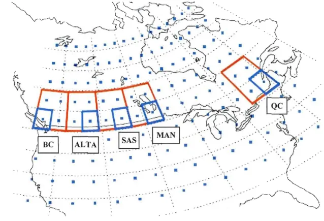
Fig. 3 shows a map of Canada with aIl available stations that measured daily total precipitation in at least sorne part of the period 1971-1990. Because of the relatively good spatial coverage, 5 different zones across Canada are selected for the analysis. A total of 10 regions are considered, 5 including one CGCM grid point and 5 including four CGCM grid points, indicated in the Fig. 3 with blue and red boxes respectively. Boundaries in latitude and longitude for ail regions are presented in Table 2. Each zone is designated with the abbreviation of the province to which it belongs: BC for British Columbia, ALTA for Alberta, SAS for Saskatchewan, MAN for Manitoba and QC for Quebec. The name of each region is then completed by adding a digit that establishes the number of CG CM grid points including in the region (e.g., BC.l is the region that belongs to British Columbia which size is one CGCM grid-box). Fig. 4 shows each region separately with the topography in col our filled contours as represented in the CRCM. BC region (BC.l and BCA) is characterized by complex topography from the Rocky Mountains and also may be influenced by land-sea interactions near the Vancouver area. ALTA region is also characterized by complex topography but in the leeward side of the Rocky Mountains. SAS, MAN and QC regions show a relatively simple topography, although SAS could be influenced by topography of the Rocky Mountains due to its proximity and the strong western flow characteristic of mid latitudes.
It is important to note that the horizontal distribution of stations within each region is not uniform. A more homogeneous distribution is generally found in regions including only one CGCM grid point than in those including four CG CM grid points. Also, for both sizes of regions, MAN and QC zones seems to show more heterogeneous horizontal distribution than the others zones. These differences could have an impact in the estimation of the spatiaJ average precipitation rate.
Fig. 5 shows the number of stations in e~ch region as a function of time in the period 1961 1990, and Table 3 indicates minimum and mean values of the number of stations within each region. Regions defined by a single CGCM grid-box (four CGCM grid-box) includea minimum of 70 (151) rain gauges per day du ring the period 1971-1990, exceeding by a factor 5 the minimum proposed by Osborn and Hulme (1997). It is interesting to note that aU regions present an annual cycle in the number of stations, with a minimum during winter and
27
a maximum in summer. Differences between both seasons are on the order of 15 stations except for ALTA region where it reaches approximately 80 stations. Interannual variations are also important and some regions indicate a significant increase in the density of stations from 1961 to 1971 and, for this reason, the period 1971-1990 is selected with the aim of increasing the confidence of regional daily precipitation estimations.
Table 3 also shows the number of model grid points within each region. The number of CRCM grid points within a single CGCM grid box is variable because of the use of the polar stereographie conformai projection in the CRCM.
4.2. Temporal and spatial scales of analysis
As discussed in section 2.2, a direct comparison between an RCM, a GCM and observed values can be properly done only when quantities are equivaJent for the three sources of data. By equivalent, here it is meant that the evaluation is carried out at scales that are greater or equal than that of the coarser resolution model or observation system. In our case, the CGCM defines the minimum area at which to perform the comparison and this corresponds to one CGCM grid box. The choice of the coarser resolution as the unit of comparison forces us to transform high-resolution data into lower resolution. Assuming that climate models produce area-average estimations of precipitation (see section 2.2), upscaling RCM and observed results to the GCM level simply consists in computing the spatial-average of ail grid-points and stations data within each GCM grid box. Similarly, the fact that the GCM cumulative precipitation data was archived at 24-hour intervals forces to carry the comparison at this time scale, thus discarding shorter time interval information.
For each source of data, let us denote with PR=PRijr the mean precipitation rate of thej'h
day for the
/h
point within the region r of interest. In our case,} E fI,}] with j=7300 since we consider 20 years between 1971 and 1990 with 365 values each. The spatial average for each region r, in day}, is simply computed as:1 1
(PR). = - "PR. .. (1)
Jr 1 LJ IJr
Î=l
where the subscript i represents stations or model grid points in each region r. Values of 1 for each data set and region are presented in Table 3. In the case of simulated data, the total number of grid points within each region is constant with time (e.g., 1 = constant). On the
other hand, for observed data, ail stations available each day are included in the estimations of the area-averaged precipitation rate, and the total number of stations depends on the completeness of the archive (i.e., 1 = lûJ). The minimum and mean values of lûJ during the period 1971-1990 for each region are presented in Table 3.
For observed data, as was discussed in section 2.2, the accuracy of the estimation of the area average is related to the number of stations, their spatial distribution, weather regime, etc. In the case of the CRCM data, the upscaling is done directly because the nature of data (area average output) from the CGCM and of the CRCM is the same. We only have to make sure that in the calculation of the eq. (1), CRCM grid boxes overlap the CGCM region.
4.3. Statistical analysis tools
As was discussed in section 2.4, time-averaged variables may not be the ideal method to evaluate model performance. For this reason, an assessment of daily statistics derived from the calculation of intensity frequency distributions is performed in addition to the study of monthly mean values.
4.3.1. Monthly mean values
Following the notation defined above, monthly mean values for each time series are calcuJated in the usual form:
29
1 1990
(PR) = - "'(PR) (2)
mr 20 LJ myr' y=1971
where (PR)myrcorrespond to the mean precipitation rate of the month m E [1,12] for the year
y E [1971,1990] in the region r. In the same way we can calculate seasonal mean
precipitation rate values ((PR)syr) by averaging over 3-month periods.
Simulated seasonal errors are calculated as departures from observed seasonal mean values and then normalized by the observed values, so that results from different regions, seasons and weather regimes could be compared in terms of relative differences. Normalized seasonal deviations (NSD) could then be expressed as
( pR)mOd (pR)obs
NSD mod = sr - sr (3)
sr (PR)::s'
To determine if NSD exhibits substantial differences for a particular region or weather regimes, the average of absolute values of NSD across seasons and regions respectively is calculated. Absolute values (ANSD = INSDI) are used in the calculation of mean values to avoid compensations between regions and seasons with NSD of different signs.
4.3.2. Estimation o/precipita/ion intensity distributions
Intensity distributions of simulated daily precipitation have been used in several studies (e.g., Durman et al., 2001; Gutowski et al., 2003; Perkins et al., 2007; Boberg et al., 2007). In al! of these studies, the bins width of precipitation used to construct the histograms were kept constant. In this work, we have chosen variable bin sizes that vary logarithmically in order to account for the reduction on the number of events with increasing intensity. Histograms for each time series are constructed from the frequency of occurrence of events function defined in the folJowing way: