ÉVALUATION DE LA VALEUR AJOUTÉE ASSOCIÉE À UNE
AUGMENTATION DE LA RÉSOLUTION HORIZONTALE DU MODÈLE
RÉGIONAL CANADIEN DU CLIMAT VERSION 5 POUR LA PRODUCTION
DE PRÉCIPITATIONS VERGLAÇANTES SUR LE NORD-EST DE
L'AMÉRIQUE DU NORD.
MÉMOIRE
PRÉSENTÉ
COMME EXIGENCE PARTIELLE
DE LA MAÎTRISE EN SCIENCES DE L'ATMOSPHÈRE
PAR
MÉDÉRIC ST-PIERRE
UNIVERSITÉ DU QUÉBEC À MONTRÉAL Service des bibliothèques
Avertissement
La diffusion de ce mémoire se fait dans le respect des droits de son auteur, qui a signé le formulaire Autorisation de reproduire et de diffuser un travail de recherche de cycles supérieurs (SDU-522 – Rév.01-2006). Cette autorisation stipule que «conformément à l’article 11 du Règlement no 8 des études de cycles supérieurs, [l’auteur] concède à l’Université du Québec à Montréal une licence non exclusive d’utilisation et de publication de la totalité ou d’une partie importante de [son] travail de recherche pour des fins pédagogiques et non commerciales. Plus précisément, [l’auteur] autorise l’Université du Québec à Montréal à reproduire, diffuser, prêter, distribuer ou vendre des copies de [son] travail de recherche à des fins non commerciales sur quelque support que ce soit, y compris l’Internet. Cette licence et cette autorisation n’entraînent pas une renonciation de [la] part [de l’auteur] à [ses] droits moraux ni à [ses] droits de propriété intellectuelle. Sauf entente contraire, [l’auteur] conserve la liberté de diffuser et de commercialiser ou non ce travail dont [il] possède un exemplaire.»
Avant toute chose, j'aimerais remercier ma directrice Julie Thériault et ma codirectrice Dominique Paquin. Ce projet n'aurait jamais été possible sans leur contribution. Merci d'avoir répondu à mes multiples questions, d'avoir proposé vos idées et surtout de m'avoir réorienté vers le droit chemin lorsqu'il a été nécessaire.
Merci également à tous mes collègues et professeurs. Votre aide et surtout votre sourire ont toujours été de mise. Merci spécialement à Eva Monteiro qui, littéralement, a toujours eu sa porte ouverte.
Un merci tout particulier à tous mes amis en dehors de l'université ainsi qu'à toute ma famille, soit: France Létoumeau, Michel St-Pierre, William St-Pierre et Sandrine St-Pierre. Sans nécessairement s'en rendre compte, ils m'ont permis de réaliser ce projet.
Finalement, il est important de mentionner que les données du MRCC5 ont été générées et fournies par Ouranos. Le MRCC5 a été développé au Centre ESCER de l'UQAM en collaboration avec Environement et Changement Climatique Canada (ECCC). Les calculs du MRCC5 ont été effectués sur le superordinateur guillimin de l'Université McGill, géré par Calcul Québec et Calcul Canada. L'exploitation du supercalculateur est financée par la Fondation canadienne pour l'innovation (FCI), le ministère de l'Économie, de la science et de l'innovation du Québec (MESI) et le Fonds de recherche du Québec - Nature et technologies (FRQNT).
LISTE DES FIGURES ... VII LISTE DES TABLEAUX ... XI LISTE DES ABRÉVIATIONS, SIGLES ET ACRONYMES ... XIII LISTE DES SYMBOLES ET DES UNITÉS ... XV RÉSUMÉ ... XVII CHAPITRE!
INTRODUCTION ... 1 CHAPITRE II
INFLUENCE OF THE MODEL HORIZONTAL RESOLUTION ON
ATMOSPHERIC CONDITIONS LEADING TO FREEZING RAIN IN REGIONAL CLIMATE SIMULATIONS OVER NORTHEASTERN NORTH AMERICA ... 9 Abstract
2.1 Introduction
2.2 Experimental Design
2.2.1 Model description ... . 2.2.2 Simulations
2.2.3 Definition of freezing rain events 2.2.4 Data analysis
2.3 Climatology
2.3 .1 Simulated precipitation
2.3.2 Annual and seasonal median number ofhours 2.3 .3 Monthly variation of freezing rain
2.3 .4 Climatology in the St. Lawrence River Valley 2.4 Event based corn pari son ...
11 13 16 16 18 18 19 21 21 22 23 24 24 2.4.1 Number of freezing rain events ... 24
Vl
2.4.2 Captured single events 26
2.4.3 Observed events missed by the simulations ... 26
2.4.4 Specific cases study ... 27
2.5 Conclusions ... 28 FIGURES ... 33 TABLEAUX 49 CHAPITRE III CONCLUSION ... 51 APPENDICE A ADDITIONAL FIGURES MENTIONED IN CHAPTER 2 .. 55 CHAPITRE IV
Figure Page
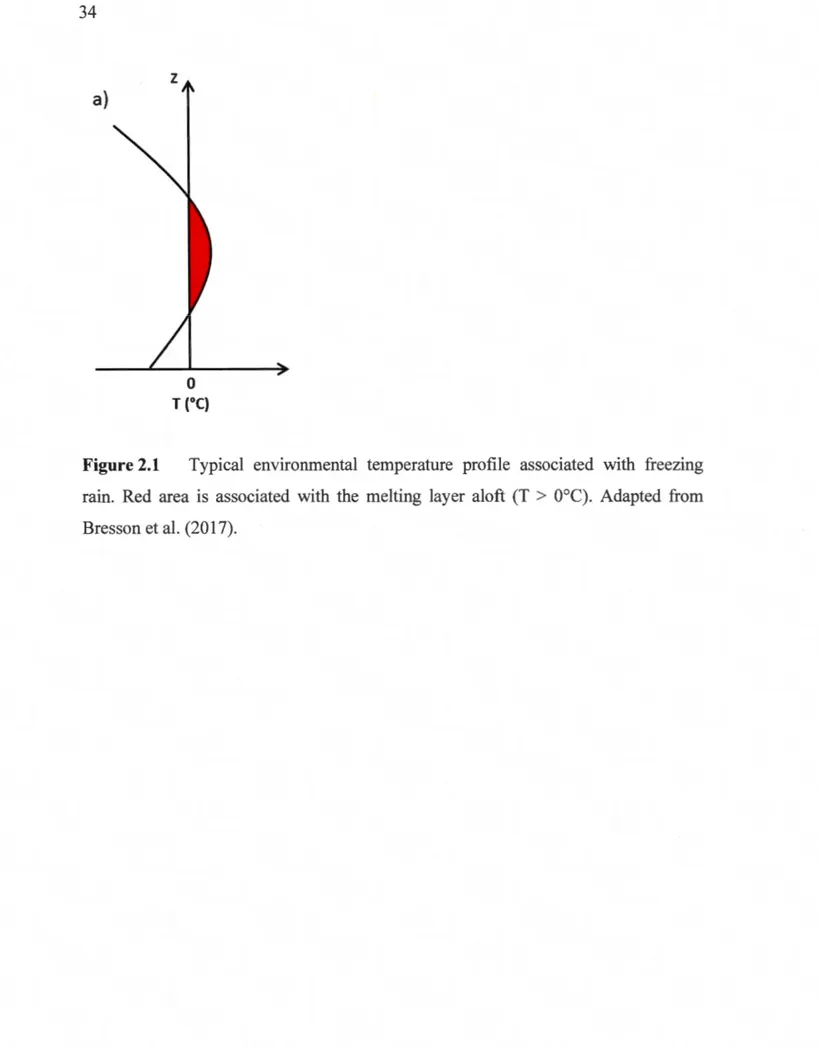
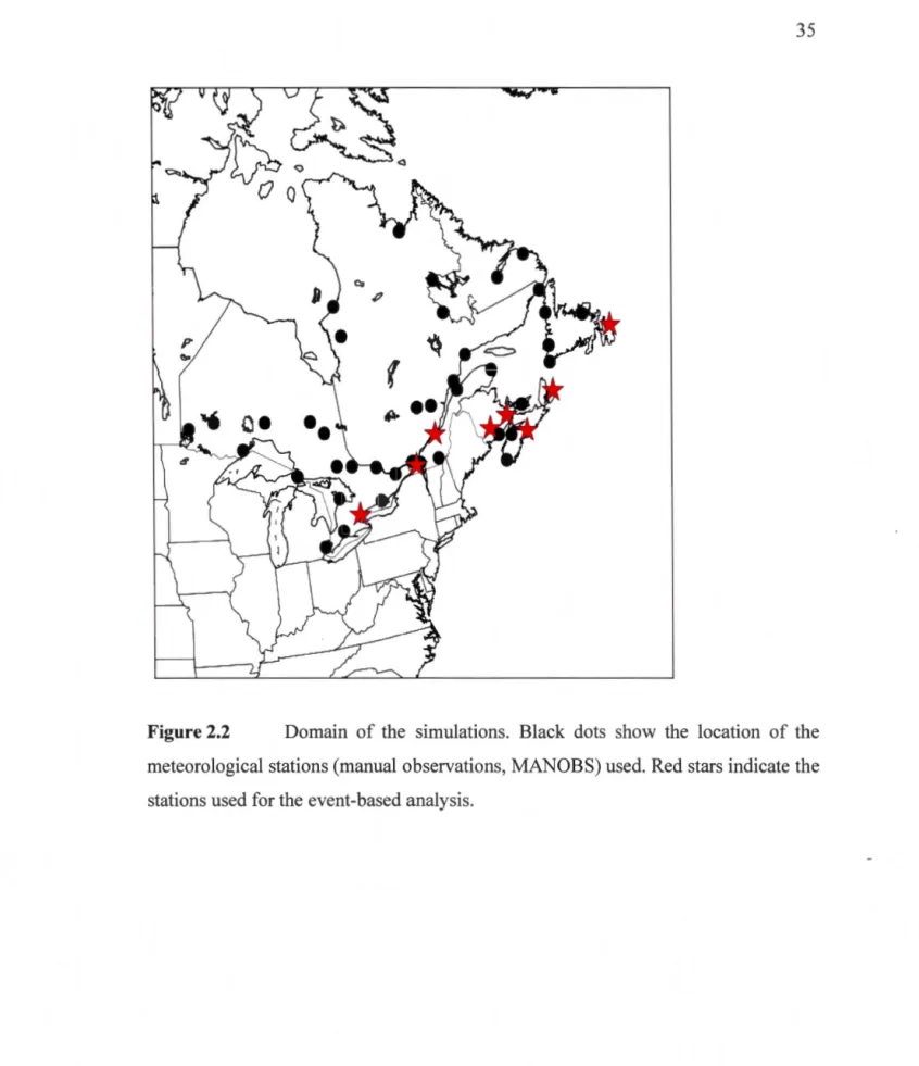
Figure 2.1 Typical environmental temperature profile associated with freezing rain. Red area is associated with the melting layer aloft (T > 0°C). Adapted from Bresson et al. (2017) ... 34 Figure 2.2 Domain of the simulations. Black dots show the location of the
meteorological stations (manual observations, MANOBS) used. Red stars indicate the stations used for the event-based analysis ... 35 Figure 2.3 Schematic diagram showing the method use to diagnose the events that
were not reproduced by the simulations. This method has been applied for every output range between 12 h before and after the missed observed events. This decision tree is based on the assumptions in Bourgouin (2000) so
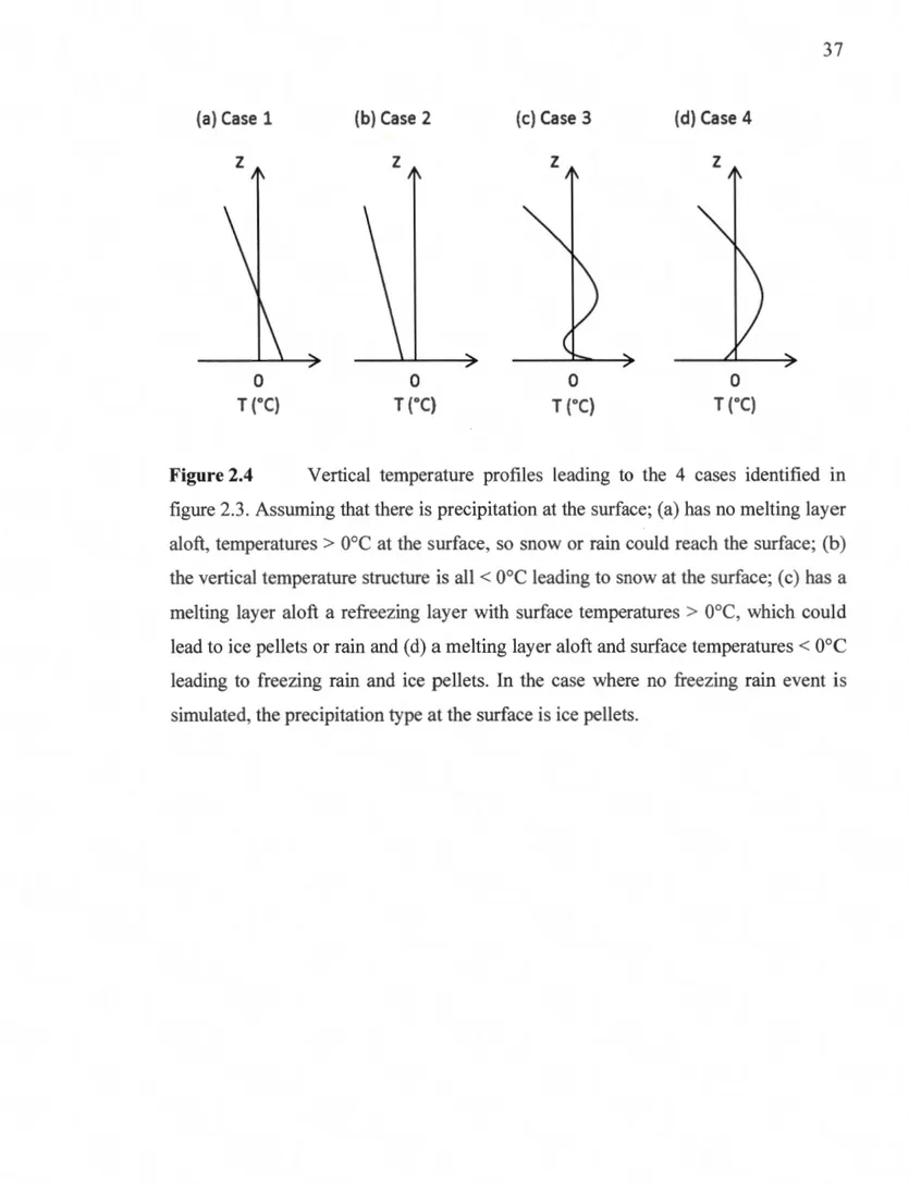
freezing rain can only be diagnose when the surface temperature is < 0°C .. 36 Figure 2.4 Vertical temperature profiles leading to the 4 cases identified in figure
2.3. Assuming that there is precipitation at the surface; (a) has no melting layer aloft, temperatures > 0°C at the surface, so snow or rain could reach the surface; (b) the vertical temperature structure is all < 0°C leading to snow at the surface; ( c) has a melting layer aloft a refreezing layer with surface temperatures > 0°C, which could lead to ice pellets or rain and ( d) a melting layer aloft and surface temperatures < 0°C leading to freezing rain and ice pellets. In the case where no freezing rain event is simulated, the
precipitation type at the surface is ice pellets ... 37 Figure 2.5 Precipitation bias with respect to CRU for (a, b, c) winter (DJF) and (d,
e, f) spring (MAM) at 0.44°, 0.22° and 0.11° horizontal resolutions over northeastem North America for the period from 1980 to 2010 ... 38 Figure 2.6 Annual (a to d) and Seasonal median occurrences of freezing rain [h]
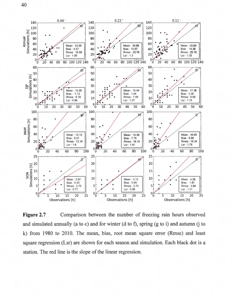
during (e to h) winter (DJF), (i to 1) spring (MAM), (m top) summer (JJA) and ( q to t) autumn (SON) for the CRCM5 simulations ( column 1 to 3) and the observations (column 4) from 1980 to 2010 ... 39 Figure 2.7 Comparison between the number of freezing rain hours observed and
simulated annually (a to c) and for winter ( d to f), spring (g to i) and autumn
G
to k) from 1980 to 2010. The mean, bias, root mean square error (Rmse)vm
and least square regression (Lsr) are shown for each season and simulation. Each black dot is a station. The red line is the slope of the linear regression ...
40 Figure 2.8 Temporal distributions of freezing rain simulated with CRCM5 at 0.11°,
0.22° and 0.44° horizontal resolutions and observed for 8 locations for the period from 1980 to 2010. The errors with respect to the observations are indicated in the top left corner ... 41 Figure 2.9 Seasonal climatology of the St. Lawrence River Valley for the period
from 1980 to 2010. (a) The 448, 112 and 28 grid cells selected for the 0.11°, 0.22° and 0.44° simulations, respectively. The red star is Montréal and the blue star is Québec City. (b) Average number of freezing rain hours per grid cell for the grey zone in (a) ... 42 Figure 2.10 Freezing rain event distributions for the 8 Canadian stations simulated
at 0.11°, 0.22° and 0.44° as well as observations for the period from 1980 to 2010 ... 43 Figure 2.11 Number of freezing rain events per year for the 8 stations simulated at
0.11°, 0.22° and 0.44 ° as well as observations for the period from 1980 to 2010. (a) is the number of short and (b) is the number oflong duration
events. 44
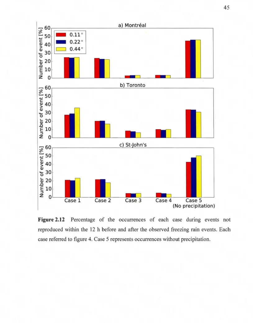
Figure 2.12 Percentage of the occurrences of each case during events not
reproduced within the 12 h before and after the observed freezing rain events. Each case referred to figure 4. Case 5 represents occurrences without
precipitation ... 45 Figure 2.13 Time evolution of the precipitation types at the surface during the
January 1998 Ice Storm simulated by CRCM5 at (a) 0.44°, (c) 0.22° and (e) 0.11° horizontal resolutions for the nearest points from Montréal (YUL). The time evolution of the vertical temperature profiles simulated by CRCM5, for the same period, is shown for the (b) 0.44 ° ( d) 0.22° and (f) 0.11°
simulations. The bars are the total amount of precipitation, which indicates the amount of each precipitation type, during the course of the simulated event. Observed types of precipitations are also included in (a) ... 46 Figure 2.14 Total accumulated freezing rain during the January 1998 Ice storm and
its distribution over southem Québec and, for the simulations, northeastem United States. The grid cell including the Montréal airport (YUL) is indicated by the black square and circle ... 4 7 Figure A. l Mean daily precipitation according to the CRU database for (a) winter
Figure A.2 Number of freezing rain hours per year for the 8 stations simulated at 0.11°, 0.22° and 0.44° as well as observations. (a) is associated to short and (b) to long duration events ... 56 Figure A.3 Median temperature profiles associated with all freezing rain events that
were not reproduced by the simulations. (a, d, g) are for Montréal, (b, e, h) are for Toronto and (c, f, i) are for St. John's at 0.11°, 0.22° and 0.44°, respectively ... 57 Figure A.4 Time evolution of the precipitation types at the surface during the
December 2013 ice storm simulated by CRCM5 at (a) 0.44°, (c) 0.22° and (e) 0.11° horizontal resolutions for the nearest points from Toronto (YYZ). The time evolution of the vertical temperature profiles simulated by CRCM5, for the same period, is shown for the (b) 0.44° (d) 0.22° and (t) 0.11°
simulations. The bars are the total amount of precipitation, which indicates the amount of each precipitation type, during the course of the simulated event. Observed precipitations are also included in (a) ... 58 Figure A.5 Total accumulated freezing rain simulated during the December 2013
ice storm and its distribution over southem Ontario. The grid cell including the Toronto airport (YYZ) is highlighted in black. ... 59
Tableau Page Tableau 2.1 Percentage of observed events that were simulated at 0.11°, 0.22° and
CORDEX Coordinated Regional Climate Downscaling Experiment
CLASS Canadian LAnd Surface Scheme
CMC Centre météorologique canadien
CPCM convection-permitting climate model
CRCM5 Canadian Regional Climate Model, version 5
CRU Climatic Research Unit
ECCC Environnement et Changement climatique Canada
ESCER (Centre pour l') -étude et la simulation du climat à l'échelle régionale
GEM Global Environment Multiscale
GCM global climate model
LD long duration
MANOBS MANual OBServations MCG modèle de circulation générale
MESI Ministère de l'Économie, de la science et de l'innovation du Québec MRC modèle régional du climat
XlV
MRCC5 Modèle régional canadien du climat, version 5
NARCCAP North American Regional Climate Change Assessment Program
RCM regional climate model
h y d 0
oc
hour year daydegree of latitude and longitude
Les épisodes de pluie verglaçante peuvent conduire à des conditions dangereuses et interrompre, par exemple, les réseaux électriques. Or, il est difficile de prévoir l'occurrence de pluie verglaçante, car celle-ci est formée à des températures oscillant autour de 0°C. De plus, cette occurrence est influencée par les changements climatiques. Quelques études ont été menées sur les changements futurs associés à la pluie verglaçante avec des modèles de circulation générale (MCG), ayant une résolution horizontale grossière (~200 km). Ces études ont suggéré une migration générale de la pluie verglaçante vers le nord. Récemment, une première étude a testé la capacité de la cinquième version du Modèle régional canadien du climat (MRCC5) à reproduire, en climat courant, les conditions atmosphériques formant la pluie verglaçante en surface, utilisant une résolution horizontale de 0.11°. Puisque la plupart des simulations climatiques régionales sont disponibles à une résolution horizontale de 0.44°, il est nécessaire d'évaluer la capacité des modèles climatiques régionaux à reproduire les conditions atmosphériques propices à la formation de pluie verglaçante, en débutant par une étude comparative des simulations utilisant une méthode diagnostique implémentée dans le modèle (en ligne). Les outils utilisés seront trois simulations du MRCCS pilotées par les réanalyses ERA-Interim sur l'est de l'Amérique du Nord à 0.11°, 0.22° et 0.44° de résolution horizontale, sur une période de 36 ans (1979 à 2014), utilisant la méthode de Bourgouin. Une étude climatologique a été menée. Elle comprend le nombre d'heures annuelles et l'occurrence saisonnière de la pluie verglaçante, ainsi qu'une analyse de !'habilité des trois simulations à reproduire des événements de pluie verglaçante individuels. L'étude d'événements de verglas comprend la fréquence, la distribution des différents types de précipitations et une comparaison avec les observations. Les résultats ont montré que toutes les simulations reproduisent relativement bien la climatologie de la pluie verglaçante et que les tendances à grandes échelles sont similaires aux trois résolutions. Cependant, une surestimation du nombre d'heures et d'événements de pluie verglaçante est notée à plus haute résolution. Malgré cette surestimation,
certains maxima de pluie verglaçante sont mieux définis et situés par les simulations à résolution plus élevée, notamment dans la région de la vallée du fleuve Saint-Laurent. Ce travail montre que pour avoir une idée générale de la distribution de la pluie verglaçante, la résolution horizontale de 0.44° est suffisante. En contrepartie, pour localiser et étudier celle-ci dans une région spécifique, les simulations à 0.11° et 0.22° deviennent nécessaires. Par exemple, pour étudier l'évolution de la pluie verglaçante
XVlll
le long des lignes de distribution de courant électrique ou dans le cas d'un aéroport distinct.
MOTS-CLÉS : Pluie verglaçante, Modèle Régional Canadien du Climat, Résolution horizontale, Climatologie
INTRODUCTION
La pluie verglaçante a été répertoriée comme l'une des catastrophes naturelles les plus dévastatrices en période froide (Dore, 2003 ). Ces événements peuvent créer des situations extrêmement dangereuses pour la sécurité des citoyens des régions touchées. L'accumulation de glace sur les fils, peut endommager le réseau électrique, pouvant causer des pannes de courant majeures (Lecomte et al., 1998). Ces pannes conjointes avec des températures hivernales froides créent des situations critiques. La végétation est aussi affectée par l'accumulation de glace. Les arbres deviennent vulnérables en raison du poids de la glace sur les branches qui peuvent être endommagées ou même brisées (Irland, 2000). De plus, une partie de la nourriture servant aux animaux herbivores devient inaccessible pour une certaine période de temps si le froid persiste après la tempête, car la dure croûte de glace complique l'accès à la nourriture enfouie (Jones et al., 2001a; Millward et Kraft, 2004; Putkonen et al., 2009). Les chaussées deviennent glissantes pouvant causer des ralentissements de la circulation routière. Les trottoirs se voient recouverts de glace, menaçant la sécurité des piétons.
La tempête de verglas de janvier 1998, frappant les environs de Montréal, a été pendant longtemps la catastrophe naturelle la plus coûteuse du Canada (Risk Management Solutions, 2008), causant des dommages considérables dans le sud-est du Canada et le nord-est des États-Unis. Seuls l'inondation de Calgary (Alberta) en 2013 (Milrad et al., 2015) et le feu de Fort McMurray (Alberta) de 2016 (McDonald,
2
2016) ont été plus coûteux depuis les 20 dernières années. D'autres tempêtes ont créé d'importants dommages. Par exemple, dans la région de Toronto les compagnies d'assurances ont estimé les pertes dues à la tempête de verglas de décembre 2013 à 200 millions (Armenakis et Nirupama, 2014), en excluant les dommages associés aux arbres et aux fils électriques. De plus, récemment, le Nouveau-Brunswick a subi une tempête de verglas historique (New Brunswick Power, 2017). En janvier 2017, les travailleurs ont pris 12 jours pour rétablir le courant à~ 133 000 clients, soit ~ 1/6 de la population. Les réparations ont coûté environ 30 millions de dollars.
La pluie verglaçante se produit lorsque les précipitations ont lieu avec des températures autour de 0°C. Deux types de processus mènent à de la pluie verglaçante, tels que définis dans Stewart et al. (2015). Le premier, le plus commun, est un processus de fonte et de regel. Ce phénomène se manifeste lorsque les précipitations solides tombent au travers d'une couche de fonte (T > 0°C) en altitude et d'une couche de congélation (T < 0°C) près de la surface. En supposant que les précipitations solides fondent complètement lors de leur passage dans la couche de fonte, les gouttes ne regèleront pas en traversant la couche de congélation si la température n'est pas suffisamment froide, car les noyaux de glaciation ne sont activés qu'à des températures < -5°C (Meyers et al., 1992). La goutte surfondue gèlera par contre instantanément au contact de la surface, si celle-ci est à des températures < 0°C. Certaines régions, la vallée du Saint-Laurent au Québec par exemple, sont plus propices à ce genre de processus. Les vents du nord-est, produits par un effet de canalisation, y maintiennent l'air froid près de la surface (Roebber et Gyakum, 2003). À l'approche d'un front chaud, l'air chaud et humide en altitude provient généralement du golfe du Mexique. Il y aura donc formation d'une couche d'air chaud en altitude et d'une couche d'air froid en surface. Le deuxième processus est souvent associé à la production de bruine verglaçante, mais il est également possible de produire de la pluie verglaçante (Huffman et Norman, 1988). C'est un processus relié à la phase liquide. On observe ce phénomène lorsque les nuages sont
relativement chauds, où les noyaux glaçogènes ne sont pas activés et les gouttes d'eau surfondues ne gèlent pas et que la température de surface est < 0°C. Ce processus est souvent observé dans la région de St-John's (Terre-Neuve), qui est située à proximité de l'océan atlantique (Strapp et al., 1996). D'autres types de précipitations hivernales,
comme le grésil et la neige mouillée peuvent aussi être formés dans des conditions atmosphériques similaires au premier processus. Les mélanges de différents types de précipitations sont aussi fréquents (Stewart et al., 2015).
De nombreuses études ont pour sujet la climatologie des types de précipitations hivernales (pluie verglaçante et grésil) sur l'Amérique du Nord. Par exemple, Branick (1997), Zerr (1997), Bernstein (2000), Rabbins et Cortinas (2002) ainsi que Changnon et Karl (2003) ont produit des analyses sur les États-Unis. Laflamme et Périard (1998) se sont concentrés sur le Québec, tandis que Cortinas (2000) a exploré les environs des Grands Lacs. La région de St-John's, Terre-Neuve, a été étudiée par Strapp et al. (1996) et les Prairies canadiennes par Kochtubajda et al. (2017). Certains ont porté leurs travaux sur le Canada en général (McKay et Thompson, 1969; Stuart et Isaac, 1999). Cortinas Jr et al. (2004) ont étendu les recherches sur l'Amérique du Nord. Les études semblent en accord sur plusieurs points, tel le fait que la majorité de l'Amérique du Nord reçoit moins de 10 h de pluie verglaçante par année et que les occurrences maximales de pluie verglaçante se retrouvent sur la partie nord-est du continent. Le nombre d'heures peut être plus de 40 h par année dans la vallée du Saint-Laurent (Québec) et dans la région de St-John's (Terre-Neuve). Des travaux semblables ont également été faits sur l'Europe (Carrière et al., 2000) et le nord de l'Eurasie (Groisman et al., 2016), où l'ouest de la Russie est la région la plus touchée, atteignant jusqu'à 8 jours avec au moins 1 événement de pluie verglaçante par année.
En modélisation du climat, des études ont démontré que les modèles de circulation générale (MCG) et les méthodes statistiques peuvent reproduire de façon raisonnable les tendances climatologiques de la pluie verglaçante en Amérique du Nord (Lambert
4
et Hansen, 2011; Cheng et al., 2007). En revanche, la résolution spatiale de ces méthodes est considérée trop grossière pour réaliser une étude des événements précis de pluie verglaçante. L'utilisation de modèles régionaux du climat (MRC) à plus haute résolution a donc été proposée comme alternative aux MCG pour la simulation de la pluie verglaçante. Bresson et al. (201 7) ont démontré que la cinquième version du Modèle régional canadien du climat (MRCC5) pouvait reproduire les conditions propices à la pluie verglaçante avec une méthode diagnostique en ligne (Bourgouin, 2000) à plus haute résolution (0.11°). Bien que cette dernière étude ait été faite avec des simulations à 0.11°, les projets collaboratifs utilisant et proposant aux usagers des simulations de modèles climatiques régionaux ne disposent actuellement que de simulations produites à 0.44° dans le cadre du North American Regional Climate Change Assessment Program (NARCCAP; Mearns et al., 2009), ainsi qu'à 0.22° et 0.44 ° dans le cadre du Coordinated Regional Climate Downscaling Experiment (CORDEX; Mearns et al., 2017). À l'heure actuelle, quelques groupes de recherche à travers le monde ont commencé à effectuer des simulations à très haute résolution qui permettent de résoudre la convection, les nuages et la précipitation explicitement. Par exemple, Liu et al. (2017) ont mené des simulations sur l'Amérique du Nord pour une durée de 13 ans à une résolution~ 4 km.
Les changements climatiques (2070-2099) associés aux précipitations mixtes ont été étudiés par Matte et al. (2018) pour le Québec. Ils ont utilisé le MRCC5 piloté par les réanalyses ERA-Interim 0.75° pour la simulation historique (Dee et al., 2011), et par un GCM pour la simulation du futur. 5 différents algorithmes de typage des précipitations ont été utilisés en évaluation « off-line », soit à partir des données préalablement archivées. La simulation pour le futur est basée sur le scénario d'émission Representative Concentration Pathway 8.5 (RCP8.5) (Moss et al., 2010). C'est la première étude à évaluer les précipitations mixtes dans le futur en utilisant un MRC avec une résolution horizontale de 0.11°. Selon cette étude le nombre d'événements de courte durée (< 6 h) et leur nombre d'heures diminueront au sud et
augmenteront légèrement au nord de la province. En contrepartie, le nombre et la longévité des événements de longue durée (~ 6 h) diminueront. La migration vers le nord n'est pas notée dans le cas des événements longs (Matte et al., 2018).
Il existe plusieurs méthodes diagnostiques pour déterminer le type de précipitation à la surface. Ces méthodes sont basées sur des statistiques développées à l'aide d'observations. Elles font un diagnostic du type de précipitation à la surface à l'aide de variables météorologiques, comme, la température, la pression atmosphérique et l'humidité relative. Parfois elles sont utilisées par des centres de prévision météorologique. Parmi les méthodes existantes les plus connues, on retrouve celle de DeRouin (1973 ), qui a été utilisée opérationnellement au Centre météorologique canadien (CMC). Cet algorithme utilise seulement la hauteur, d'au plus, 3 niveaux de congélation comme prédicteur du type de précipitation et aucune température verticale n'est considérée. Cantin et Bachand (1993) utilisent les épaisseurs partielles des couches atmosphériques 1000-850 hPa et 850-700 hPa, épaisseurs directement reliées à la température moyenne de la couche. L'algorithme de Ramer (1993) utilise la température, l'humidité relative et la température du thermomètre mouillé afin de définir les couches atmosphériques les plus susceptibles de développer de la précipitation. Ces paramètres sont aussi utilisés pour calculer la fraction de glace. La méthode de Baldwin et Contomo ( 1993) est basée sur le profil atmosphérique de la température du thermomètre mouillé et sur la température proche de la surface. Ces deux paramètres sont utilisés pour déterminer l'endroit où il y aura formation de cristaux de glace, ainsi que les différents changements de phase subis au cours de leur chute vers la surface. La dernière méthode présentée est celle implémentée dans le modèle de prévision numérique GEM -Global Environment Multiscale (Côté et al., 1998), soit Bourgouin (2000). Cette méthode utilise le profil vertical de température et la hauteur de l'isotherme 0°C pour calculer le bilan d'énergie au-dessus de la surface.
6
Les schémas microphysiques offrent une seconde option pour le diagnostic des précipitations en surface. Ils impliquent des équations physiques décrivant les nuages et les précipitations (Morrisson and Milbrandt, 2015; Thompson and Eidhammer, 2014; Milbrandt and Yau, 2005). Ces méthodes sont trop exigeantes en coût de calcul sous leur forme actuelle pour les modèles de climat et ne sont utilisées de façon opérationnelle qu'en mode prévision numérique du temps. Cette charge au niveau des calculs vient du fait qu'elles tiennent compte des rétroactions thermodynamiques associées aux changements de phases. Par exemple, l'absorption (libération) de chaleur latente lorsque les flocons (gouttes) fondent (gèlent) en altitude (surface) va causer un refroidissement (réchauffement) de la couche de fonte (congélation), qui sans forçage, se rapprochera de 0°C (Stewart, 1985; Lackmann et al., 2002). Il y a également la fonte des flocons qui dépend du maximum de température de l'inversion en altitude. Stewart et King (1987) ont montré qu'une couche de fonte ayant un maximum plus chaud que 3.8°C ferait fondre les flocons (densité de 0.025 et 0.05 g cm3) de diamètre < 4 mm tandis qu'aucun flocon ne fondrait à une température <
0.8°C. Le degré de fonte influence le type de précipitation qui atteindra la surface (Thériault et Stewart, 2010).
Étant donné l'importance d'une meilleure compréhension de l'évolution future des précipitations verglaçantes, il est essentiel d'évaluer l'efficacité avec laquelle les MRC simulent les conditions atmosphériques produisant de telles précipitations. Le but de cette étude est d'évaluer le gain obtenu par une résolution spatiale plus élevée· dans la reproduction des conditions atmosphériques produisant de la pluie verglaçante à la surface. Cette étude est exécutée avec le MRCC5 (Martynov et al., 2013; Separovic et al., 2013) pour l'est du Canada. Des simulations historiques de 1979 à 2014 ont été produites à des résolutions horizontales de 0.11°, 0.22° et 0.44°.
Premièrement, une validation des simulations sera menée en comparant la climatologie de la pluie verglaçante avec celle des observations. Deuxièmement, des
études de distributions spatiales et temporelles seront effectuées. Troisièmement, une analyse des événements de pluie verglaçante a été exécutée pour 8 stations météorologiques, utilisant une définition précise d'événements de pluie verglaçante. Finalement, une analyse spécifique des tempêtes de janvier 1998 et de décembre 2013 a été menée pour les environs de Montréal et Toronto, respectivement.
Ce mémoire est organisé de la façon suivante. Le chapitre 2 est rédigé sous forme d'un article scientifique en anglais qui sera soumis à la revue Atmosphere-Ocean. La section 2.1 est l'introduction. La méthodologie comprenant la description du modèle,
des simulations, des observations ainsi que des analyses effectuées est développée dans la section 2.2. La section 2.3 montre la climatologie de la pluie verglaçante sur le domaine utilisé. Une analyse basée sur les événements de pluie verglaçante est présentée dans la section 2.4. Finalement, la section 2.5 résume les résultats. Le chapitre 3 est la conclusion en français.
INFLUENCE OF THE MODEL HORIZONTAL RESOLUTION ON
ATMOSPHERIC CONDITIONS LEADING TO FREEZING RAIN IN REGIONAL CLIMATE SIMULA TI ONS OVER NORTHEASTERN NORTH AMERICA
by
Médéric St-Pierre1*, Julie M. Thériault1, Dominique Paquin2
1
Department of Earth and Atmospheric Sciences, Université du Québec À Montréal, Montréal, Québec
2
Consortium Ouranos, Montréal, Québec
*
Corresponding author : [email protected]Freezing rain can lead to hazardous conditions that can, among other impacts,
interrupt power transportation networks. The occurrence and location of freezing rain events will likely be affected by climate changes. A few studies have been conducted on the future evolution of freezing rain with global climate models (GCMs), that have a coarse resolution (~200 km). They suggested a general northward migration of freezing rain occurrences. This current study highlights the sensitivity of studying freezing precipitations using regional climate models because they are formed in a narrow range of conditions when the temperature is near 0°C. An initial study has tested the ability of the fifth-generation of the Canadian Regional Climate Model (CRCM5) at a horizontal resolution of 0.11° to reproduce the atmospheric conditions leading to freezing precipitations. There is a need to assess the ability of regional climate models to produce atmospheric conditions leading to freezing rain at coarser resolution because most simulations are available at 0.44° horizontal resolution. The goal is to investigate the influence of the different horizontal resolutions for the simulation of atmospheric conditions leading to freezing rain using the CRCM5. Freezing rain is diagnosed using an in-line diagnostic method for precipitation partition. Three CRCM5 simulations driven by ERA-Interim reanalysis over Eastern North America at 0.11°, 0.22° and 0.44° are conducted over a period of 36 years (1979 to 2014). A climatology study, including annual, seasonal accumulated freezing rain, is conducted, as well as the ability of the three simulations to reproduce individual freezing rain events. Our analysis includes frequency, partition of different precipitation types and comparisons with observations. The results pointed out that all simulations reproduced the climatology of freezing rain relatively well and that the large-scale patterns are similar. Despite the overestimation in the number of freezing rain events at higher resolution, detailed maxima associated with freezing rain are better defined and located in simulations at higher resolution, notably in regions located in the St. Lawrence River Valley. Overall, this study highlights the challenge of producing the atmospheric conditions leading to freezing rain. Nevertheless, there is a need to use higher resolution to assess changes in freezing rain locally, which is critical for decision-making.
Freezing rain is one of the most catastrophic weather hazards occurring during the cold season in North America (Dore, 2003). Ice accumulation can damage the power network, causing power interruptions. Trees are vulnerable during these events due to the ice load over the branches. As examples, the January 1998 Ice Storm near Montréal has been reported as the third costliest natural disaster that happened in Canada (Risk Management Solutions, 2008), with considerable damage in both southeastem Canada and northeastem United States. Around 400 000 residents were without power for two weeks after the storm and it took roughly a month to restore all the electrical networks (Lecomte et al., 1998). In Toronto, the December 2013 ice storm insured losses were estimated at 200 million excluding damages to trees and wires (Armenakis and Nirupama, 2014).
Freezing rain occurs when precipitation occurs with the air temperature around 0°C. It can be formed through warm and cold rain processes (Stewart et al., 2015), although cold rain processes is the most common one at mid-latitudes. Freezing rain is generally formed when solid precipitation falls through a melting layer (T > 0°C) aloft a lower-level refreezing layer (T < 0°C). If solid precipitation melts completely, the drops will not freeze while falling through the sub-freezing layer because no (or very few) ice nuclei are activated at temperatures > -5°C (Meyers et al., 1992). The supercooled drops will freeze instantly upon contact with the sub-freezing surface. Others winter precipitation types, such as ice pellets, can also be formed in similar atmospheric conditions. A typical temperature profile associated with these types of precipitation is shown in figure 2.1. In the case of the warm process, it is generally associated with the formation of freezing drizzle, but it is also possible to observe freezing rain (Huffman and Norman, 1988). This process is related to the liquid phase. This phenomenon occurs when the clouds are relatively warm, where the ice nucleation is absent and the supercooled water drops do not freeze and reach the subfreezing surface ( < 0°C). This process is often observed in the St. John's,
14
Newfoundland area, which is located on the Atlantic Ocean Shore (Strapp et al., 1996).
Most studies concerning freezing rain were conducted over a region in North America. The northeastern part of North America receives at least 5 h of freezing rain per year with maxima reaching > 30 h
i
1 in some areas (Cortinas Jr et al., 2004; Kochtubajda et al., 2017). Hence, the region has been the center of interest for many studies, though other studies have focused their interests on different areas of the world. The outcomes showed that Europe (Carriere et al., 2000) and Northern Eurasia (Groisman et al., 2016) undergo their fair amount of freezing rain events, but the quantities received are much less than North America. Such a worldwide phenomenon needs to be well reproduced by models to prevent risks associated with freezing precipitation events.Lambert and Hansen (2011) and Cheng et al. (2007) have demonstrated that global climate models (GCMs) and statistical methods can reproduce reasonably well the large-scale patterns of the freezing rain climatology over North America. The temporal and spatial resolutions, however, are too coarse to identify specific freezing rain events and local effects. The use of regional climate models (RCMs) with finer resolution has been proposed as an alternative to GCMs for the simulation of freezing rain. The ability of the fifth-generation of the Canadian Regional Climate Model (CRCM5) using Bourgouin (2000) in-line diagnostic method to produce atmospheric conditions leading to freezing rain using a 0.11° horizontal resolution has been successfully shown by Bresson et al. (2017). The added value of using convection-permitting climate models (CPCMs) is also currently being investigated. Sorne climate research groups have started to conduct simulations, including North America, using horizontal resolutions ::S 4 km (Liu et al., 2017) for 10 to 20 years. With this level of detail, it is possible to explicitly solve the convection and microphysical processes of clouds and precipitations are parameterized. However,
these CPCMs are currently still too costly to be used as operational climate models. To the best of our knowledge, regional climate models do not solve explicitly freezing precipitations and diagnostic methods such as Bourgouin (2000) and Benjamin et al. (2016) are still being used.
Future changes (2070-2099) in mixed precipitation, over the Québec Province using 5 different off-line precipitation-typing algorithms have been studied by Matte et al. (2018). They used the CRCM5 driven by the ERA-Interim 0.75° reanalysis (Dee et al., 2011) for the hindcast simulation and by a GCM for the simulation of the future,
under the emission scenario RCP8.5 (Moss et al., 2010). This is the first study to assess mixed precipitations in the future using an RCM at a 0.11° horizontal resolution. They found that the number of hours and events associated with short duration events ( < 6 h) will decrease in the south and slightly increase in the north of the province. For long duration events (~ 6 h), the study shows a reduction in both number of hours and events without northward migration of the freezing preci pi tation.
Given the importance of better understanding how freezing precipitation occurrence will evolve in the future, it is critical to assess how well regional climate models simulate the atmospheric conditions leading to such precipitation. Currently,
ensembles of regional climate simulations data available for users over North America are coming through the North American Regional Climate Change Assessment Program (NARCCAP; Mearns et al., 2009) at a resolution of 0.44°, and at resolutions of 0.22° and 0.44 ° through the Coordinated Regional Climate Downscaling Experiment (CORDEX; Mearns et al., 2017). On the other hand,
regional climate modelling has started to be performed with resolution :S 4 km (Liu et al., 2017) and another approach to climate projections, such as the pseudo-global warming (PG W), is being used to study changes in fine-scale processes in warmer conditions.
16
The goal of this study is to evaluate the gain of using higher spatial resolution to reproduce the atmospheric conditions leading to freezing rain at the surface. This is conducted with the CRCM5 (Martynov et al., 2013; Separovic et al., 2013) driven by ERA-Interim reanalyses over eastern Canada. Historical simulations from 1979 to 2014 have been conducted at 0.11°, 0.22° and 0.44° horizontal resolutions.
The paper is divided as follows. The experimental design including a description of the CRCM5, the simulations and observations, the diagnostic methods as well as the methodology is given in section 2.2. Section 2.3 addresses the freezing rain climatology with a spatial and temporal approach. Difference between resolutions to compare small and long duration freezing rain events are discussed in section 2.4. Specific long duration events have also been studied in section 2.4. Conclusions are in section 2.5.
2.2 Experimental Design
2.2.1 Model description
The fifth-generation of the Canadian Regional Climate Model (CRCM5; Martynov et al., 2013; Separovic et al., 2013) developed at the Centre pour l'Étude et la Simulation du Climat à l'Échelle Régionale (ESCER) at the Université du Québec à Montréal (UQÀM) in collaboration with Environment and Climate Change Canada (ECCC) has been used. lt is based on a limited-area version of the Global Environment Multiscale (GEM) model (Côté et al., 1998), that is used at ECCC for Numerical Weather Prediction (Côté et al., 1998). GEM is a grid-point model based on a two-time-level semi-Lagrangian (quasi) fully implicit time .discretization scheme. lt includes a terrain-following vertical coordinate based on hydrostatic pressure (Laprise, 1992) and the horizontal discretization based on a rotated latitude-longitude, Arakawa C grid (Arakawa and Lamb, 1977). The nesting technique employed in CRCM5 is derived from Davies (1976). lt includes a 10-point wide halo zone along the lateral boundaries for the semi-Lagrangian interpolation and a
10-point sponge zone for a gradua! relaxation of all prognostic atmospheric variables
toward the driving data along the lateral boundaries.
The parameterizations of CRCM5 are essentially the same as GEM. lt includes: deep
convection from Kain and Fritsch (1990), shallow convection issued from a transient version of Kuo (1965) described in Bélair et al. (2005), large-scale condensation
(Sundqvist et al., 1989), correlated-K solar and terrestrial radiation (Li and Barker,
2005), subgrid-scale orographie gravity waves drag (McFarlane, 1987), the low-level
orographie blocking parameterization (Zadra et al., 2003) modified by Zadra et al.
(2012) and the planetary boundary layer parameterization (Benoit et al., 1989; Delage
and Girard, 1992; Delage, 1997) modified in Zadra et al. (2012), introducing
turbulent hysteresis. Unlike the NWP version of GEM, the Canadian land-surface
scheme version 3.5 (CLASS; Verseghy, 1991, 2008) and Flake lake models (Mironov
et al., 2010) are used.
An in-line surface precipitation diagnostic method, Bourgouin (2000), allows the
partition of freezing rain and ice pellets. This method is called the area method. The criteria diagnosing precipitations have been developed and validated by Bourgouin
(2000) with data from the 1989-1990, 1990-1991 and 1991-1992 cold seasons over
North America. 1t is currently operational in CRCM5 and used at ECCC for medium term forecasting of precipitation types. The method compared the areas bound by the
0°C isotherms and the temperature associated with both the warm layer aloft and the
cold layer near the surface. The algorithm discriminates snow, rain, freezing rain and
ice pellets by comparing these areas. The method also has some limitations. lt has
been developed with a limited number of 54 vertical temperature profiles. Also, it
only solves for freezing rain and ice pellets formed through cold processes. Warm
rain processes are neglected, which means that observed freezing rain during those
18
example, are prone to freezing rain formation through warm processes (Roberts and Stewart, 2008; Kochtubajda et al., 2017).
2.2.2 Simulations
Three CRCM5 simulations with different horizontal resolutions of 0.11°, 0.22° and 0.44 ° are used. Each one has a vertical resolution of 56 levels from the surface to 10 hPa ( ~ 3 0 km) up in the atmosphere. They were performed over northeastem North America with respective free domains exclusive of 40 points sponge and halo zones are composed of 300 x 300, 160 x 160 and 76 x 76 grid cells. Figure 2.2 shows the region of interest for the simulations. The time step is 5, 10 and 20 minutes for the 0.11°, 0.22° and 0.44° simulations, respectively, and variables are archived every 3 h,
but total precipitation is archived every hour. The driving data are the ERA-Interim 0.75° reanalysis (Dee et al., 2011), which are available every 6 h for atmospheric variables and daily for ocean data. The simulations covered a 36-year period starting in January 1979 and ending in December 2014, the first year being discarded as spin-up time. Finally, no spectral nudging is applied in the se simulations.
2.2.3 Definition of freezing rain events
Surface MANual OBServations (MANOBS) are provided hourly by ECCC for 77 meteorological stations over eastern Canada. Only the stations with at least 30 out of 35 years of data for the period from 1980 to 2014 are used, so after the data quality control described in Bresson et al. (2017), only 48 stations remain (figure 2.2). Furthermore, most analyses are conducted from 1980 to 2010 due to data availability. To conduct the event-based analysis, 8 stations indicated in figure 2.2 were selected. These are stations where high amounts of freezing rain are reported annually (~ 30h) or are associated with the main cities of eastem Canada, which are Toronto (Ontario),
Montréal (Québec), Québec City (Québec), Halifax (Nova Scotia), St. John's (Newfoundland), Fredericton (New Brunswick), Moncton (New Brunswick), and Sydney (Newfoundland). Observations also have limitations, such as their reliability
due to the manual observations and the small number of operational stations.
Furthermore, MANOBS only provides occurrences of precipitation.
A freezing rain event is defined as follows. The event starts at the first recorded observation or simulation of freezing rain and ends after more than 6 h without freezing rain. CRCM5 provided information on freezing rain on a 3 h basis. Because the model has a tendency to overproduce very light precipitation at the surface, a threshold of 1 mm d-1 of freezing rain has been determined to eliminate negligible amounts. The same threshold value was used in Lambert and Hansen (2011) with GCMs. For each given period of 3 h with precipitation greater than this threshold, a 3 h freezing rain duration is added to the event. Consequently, events duration will always be a multiple of three.
To be consistent and avoid artificial overestimation, the observations have been
treated similarly. The observations were divided in 3 h period as in Bresson et al. (2017). The closest grid cell to each meteorological station was selected for the 3 simulations and compared with observations.
Freezing rain events were then divided into two categories. The short duration (SD) events will be defined as::::; 6 h and therefore, long duration (LD) events will last > 6 h. This definition of the freezing rain event is similar to the one in previous studies, such as Ressler et al. (2012) and Matte et al. (2018). They consider SD event as< 6 h. In our definition, we include the 6 h events in the SD events category because of the lower frequency (3 h) outputs. This definition allows consideration of at least 2 time steps (one in each archive) for SD events.
2.2.4 Data analysis
20
First, the simulated precipitation biases over the domain were quantified. Subsequently, a climatological study was conducted. In particular, the seasonal average, the spatial and the temporal distributions of freezing rain were investigated using the median annual hours. Precipitation amounts were compared to the Climate Research Unit (CRU) database (Harris et al., 2014).
Second, the difference and similarities among the model simulations were assessed through two different analyses. First, the occurrences of freezing rain such as the number of events per year were compared with observations. Second, the ability of the model simulations to reproduce past observed freezing rain events within a given time range was calculated. The method considered only the closest grid cell, in each
simulation, associated with a given meteorological station. lt is called the 1-point
analysis. Using this method, observed events are considered reproduced if 3 h of freezing rain is simulated within a range of 12 h before and after the observed event. Similar outcomes were obtained performing a second analysis with more grid cells ( ~ 1 OO lrni2).
Third, following the 1-point analysis, a thorough analysis of the atmospheric conditions of all missed freezing rain events were conducted. Three parameters are necessary to diagnose freezing rain, which are the minimum amount of precipitation,
the melting layer aloft (T > 0°C) and the below 0°C surface temperature. All 3
parameters are investigated for each output frequency ranging from 12 h before and after the event following the decision tree show in figure 2.3. The anal y sis led to 4
possible vertical temperature structures defined in figure 2.4. These are associated
with different types of precipitation at the surface. Cases 1, 2, 3 and 4 would lead to
(1) rain or snow, (2) snow only, (3) ice pellets or rain and (4) freezing rain or ice pellets. Since the cases are analyzed when there is no freezing rain (missed events ),
case 4 is always associated with ice pellets. Finally, Case 5 (not shown) occurred with
Finally, since the climatology depends on all single events occurring annually,
specific events were selected and examined in detail to quantify the ability of the model to reproduce those events. The selected events are the January 1998 Ice Storm in the Montréal area and the ice storm that occurred in December 2013 in the Toronto area. The analysis includes the temporal evolution of precipitation types and temperature at the surface, vertical temperature structure and the spatial distribution.
2.3 Climatology
The ability of CRCM5 to reproduce the freezing rain climatology over a period of 31
years (1980-2010) was evaluated. The climatology of total precipitation during winter and spring was investigated followed by the spatial and temporal distributions of freezing rain. To close this section, special attention will be brought to the St. Lawrence River Valley.
2.3.1 Simulated precipitation
The CRCM5 simulated precipitation biases with respect to the CRU database, over land, at the three horizontal resolutions during winter (DJF) and spring (MAM), when most of the freezing rain occurs, are shown in figure 2.5. The CRU precipitation fields are shown in figure A.1 for both seasons. The three simulations produced an
overall wet bias over the whole domain. The bias is of the order of 0.53, 0.47 and
0.44 mm d-1 during MAM and 0.29, 0.31 and 0.30 during DJF for the 0.11°, 0.22°
and 0.44° simulations, respectively. The southern part of the domain shows a dry bias that seems to be related to the proximity of the boundary. For this reason, this region will be excluded from all future analysis. The largest maxima were near the Great
Lakes with values up to 1.50 mm d-1• This wet zone was broader with increasing
resolution for MAM, but steady during DJF. East of the Lake Superior, the three simulations produced the same dry region compared to the observations. Similarly,
22
A dry region was also produced by the 0.11° simulation in southem Newfoundland for both DJF and MAM.
The freezing rain occurrences will likely be influenced by these wet biases produced by all three simulations. The overestimation of the total precipitation may cause an overestimation of the total amount of freezing rain as it is directly related to the total amount of precipitation.
2.3 .2 Annual and seasonal median number of hours
The median annual hours of freezing rain simulated and observed during the 31-year period from 1980 to 2010 is shown in Fig. 2.6 (a to d). The means, biases, root means square errors (rmse) and least square regression are shown in Fig. 2. 7 for the 48 stations. Summer (JJA) has been excluded from the scores due to the absences of freezing rain at the stations for this season. As the horizontal resolution increases,
local maxima of freezing rain were better defined. For example, a clear local maximum was reproduced along the St. Lawrence River Valley, on the northem shore of Québec, in the center of New Brunswick and on the Atlantic Coast at 0.11°
and 0.22° resolutions. Nonetheless, comparing the observations to the closest point in each simulation, the general overestimations (bias) reach a number of 33% (14.38 h),
30% (10.57 h) and 8% ( 4.57 h) for the 0.11 °, 0.22° and 0.44 °, respectively (fig 2. 7a-c ). The number of hours of freezing rain in7a-creased with in7a-creasing horizontal resolution, as well as the general overestimation.
The occurrence of freezing rain varied significantly with the seasons (Fig. 2.6e-t). During winter (DJF), most of the region south of the 50° latitude was affected by freezing rain. This area extended farther north during spring (MAM) and, only along the northem coast of Québec and southem Baffin Island during summer (JJA). During winter, the maxima were located in the St. Lawrence Ri ver Valley. These maxima increased with increasing resolution in both covered area and occurrences
similar as for spring but with much smaller amounts (~40%). The ground being warmer in autumn than spring may explain the lower occurrences. Spring and winter occurrences of freezing rain were the highest, for all simulations, according to the 48 grid cells in each simulation (fig 2.7). However, the simulations differ from the observations during spring where the biases are 5.31, 7.75 and 8.88 h for the 0.44°,
0.22° and 0.11° simulations, respectively, whereas the biases are -1.12 (0.43), 1.44 (0.69) and 3.38 h (1.81 h) during winter (autumn).
Overall, the annual and seasonal spatial distributions of freezing ram were comparable to the observations at all resolutions. Occurrences during sprmg are overestimated in each simulation, but for the other seasons, they are closer to the observations. Local maxima were better defined at higher resolution, such as in the St. Lawrence River Valley. On the other hand, the occurrences of freezing rain were higher with increasing resolution compared to the observations, leading to a larger overestimation at higher resolution.
2.3.3 Monthly variation of freezing rain
The temporal distributions of freezing rain for 8 locations are shown in figure 2.8. For the Atlantic locations, 4 of the 5 (Moncton, Halifax, Fredericton, Sydney and St. John's) had a maximum occurrence during March or April, for both simulations and observations, whereas Fredericton had no defined peak. On the other hand, in the St. Lawrence River Valley (Montréal and Québec City), the peak of freezing rain was instead observed during December. The simulations agreed with the observations from Québec City, but for Montréal the 0.11° and 0.22° simulations showed this peak in January. Toronto is the only region where the maximum was simulated m February, with observations showing somewhat constant values from January to March. As discussed in the previous section, the occurrences of freezing rain increased with increasing resolution, which is supported by figures 2.6 and 2. 7. Finally, the 0.44° simulation often underestimated the observations.
24
The simulations reproduced fairly well the monthly cycle of freezing rain. As the resolution increased, the occurrence of freezing rain increases in location influenced by the topography (Montréal and Québec City). A better definition allowed a better simulation of the wind channelling effect in the St. Lawrence River Valley (not shown, as in Cholette et al., 2015 and Lucas-Picher et al., 2016). This led to cold air near the surface, which is favourable condition for freezing precipitations.
2.3 .4 Climatology in the St. Lawrence River Valley
To evaluate the occurrence in the St. Lawrence River Valley, the average number of hours of freezing rain per grid cell defined in an area covering the valley were compared at all resolutions (figure 2.9). The area, shown in figure 2.9a, includes Montréal and Québec City. The selected region is a rectangle composed of 448, 112 and 28 grid cells for the 0.11°, 0.22° and 0.44° simulations, respectively. According to figure 2.6 this region was located in a freezing rain maximum.
As expécted, freezing rain was occurring essentially during winter, with ~3 to 5 times less occurrence in spring and fall (Figure 2.9b ). The number of hours increased with increasing resolution. The difference between the 0.44° and the 0.11° (0.22°) resolutions for the 31-year period are ~300 h (180 h) in winter, respectively. Finally,
the number of hours at higher resolutions (0.11° and 0.22°) is closer to observations than the coarser one (0.44°), except in autumn (SON).
2.4 Event based comparison
2.4.1 Number offreezing rain events
Freezing rain events were defined by a majority of SD events in both simulations and observations (figure 2.10). The number of events decreased with the duration, and only a few events lasted more than 30 h for the 8 stations. According to the observations SD events are 65% to 80% of the total number of events. Figure 2.11 showed the number of events per year at each station. For the western stations of the
domain (Montréal, Québec City and Toronto), the highest resolution simulations generally overestimated freezing rain events. Combining these 3 stations, LD (SD) events were simulated 46% ( 69%) and 1 % ( 51 % ) more often than observed for the 0.11° and 0.22° simulations, respectively. The model behaviour was different in the Atlantic region (Fredericton, Halifax, Moncton, St. John's and Sydney) where the highest resolutions are much doser to or underestimated the observations. For instance, LD (SD) events show 8% (-14%) and 15% (-21%) difference with the observations, for the 0.11° and 0.22° simulations, respectively. In comparison, the 0.44° simulations underestimated the LD and SD events by -9% and -23% at the Atlantic stations as well as the LD events by -33% at the western stations. The 0.11° and 0.22° simulations tend to overestimate the number of events for Montréal, Québec City and Toronto, but the results were much closer to the observations in the Atlantic area. The 0.44° simulation, however, was different because it underestimated most of the freezing rain events. This analysis was also made with the number of hours and the results are similar (see appendice Al).
The overestimation at 0.11° and 0.22° for Montréal and Québec City is most likely due to the influence of the St. Lawrence River Valley, which is better defined at higher resolution. The wind direction in the valley is better represented by a 0.11° and 0.22° horizontal resolutions as shown by Lucas-Picher et al. (2016). These are favourable conditions to sustain the sub-freezing layer near the surface due to the north-easterly flow at lower elevation due to the wind channelling effects, as well as warm and moist southerly flow aloft. As for the general underestimation at the Atlantic stations, it might be attributed to the frequent freezing rain/drizzle formation through warm processes in this region, which is a process that is not diagnosed by the Bourgouin (2000) scheme, as mentioned in the section 2.2.1, is probably a cause of this behaviour.
26
2.4.2 Captured single events
The simulations were driven by reanalysis, therefore it was reasonable to assume that freezing rain events could be reproduced. A better representation of observed freezing rain events in the St. Lawrence River Valley (Montréal and Québec City) was obtained at higher resolution (Table 2.1 ). For these two stations, the 0.11° reproduced at least 12% more LD and SD events than the 0.44°. For example, more freezing rain events were reproduced at higher resolution at Québec City while there was a larger difference between the 0.44° and 0.22° than the 0.22° and 0.11° at Montréal. The LD and SD events at Toronto and the LD events at St. John's are also slightly better reproduced ( < 11 % ) for at least one of both higher resolution simulations. Finally, no significant difference was found for the other stations.
2.4.3 Observed events missed by the simulations
The factors leading to the missed freezing rain events were investigated (figure 2.12). Recall that the method and the different cases are given in figures 2.3 and 2.4. There is no clear difference between the resolutions for this analysis, however, at Montréal, the highest resolutions reproduced more events (Table 2.1 ). There are some similarities and differences among stations. First, for all three stations, freezing rain was not produced because there was no precipitation at the surface (30-50% of all outputs). Second, when precipitation reached the surface, no freezing rain was diagnosed because the melting layer was near the surface and no refreezing layer was simulated (case 1) or because the melting layer was missing (case 2). Case 1 was the most simulated in Toronto (28 to 36%) followed by case 2 (~20%). At Montréal and St. John's both cases were equally simulated (20 to 25%). Third, only a few occurrences ( < 10%) show a melting layer aloft with warm surface temperature (>
0°C), which is the case 3, or ice pellets instead of freezing rain (case 4 ). Therefore, the main reasons associated with missed freezing rain events when the model produced precipitation were because atmospheric conditions are too cold or too warm
throughout the lower levels of the atmosphere. Indeed, the surface temperature is mainly > 2°C for case 1, whereas temperatures were generally between -8°C and -2°C for case 2 at all levels (see appendice A.3).
2.4.4 Specific cases study
Examples of specific cases were studied to assess the impact of the model resolution
on freezing rain occurrences. The 1998 Ice Storm is presented because detailed ·
observations are available (Bresson et al., 2017). This Ice Storm occurred in two phases (Henson et al., 2011). The first phase of the storm was well reproduced by every simulation according to the observations (figure 2.13 a,c,e ). All resolutions simulated freezing rain, ice pellets and snow at the beginning of the storm. During the second phase, the 0.11° and 0.22° resolutions are more comparable to observations.
The 0.44° resolution produced surface temperatures > 0°C during that phase
(figure 2.13b ), which lead to rain instead of freezing rain. Observations also
suggested that ice pellets reached the surface during the second phase, which was not
reproduced by all the simulations. This could be explained because the model simulated warmer temperatures (> 5°C) aloft. The modelled temperatures were too warm leading to complete melting of ice particles, which produced supercooled drops that froze upon impact with the surface.
The spatial distribution of the accumulated amount of freezing rain during the storm has been investigated (figure 2.14). The maximum amount has been reproduced
farther west by the 0.11° (Bresson et al., 2017) and 0.22° resolutions and even farther
northwest in the 0.44 ° simulation, which explains the occurrence of rain in the second phase of the storm. All simulations reproduced the precipitation types and amounts well, even if all resolutions simulated the maximum of intensity farther west. The 0.11° and 0.22° resolutions, however, better reproduced the location and the key features with respect to observations.
28
Finally, the major ice storm that occurred in the Toronto area in December 2013 was also studied (see appendice A.4 and A.5). The evolution of precipitation types at the surface is mainly freezing rainas reported by the observations (Figure A.4a). At 0.11° resolution, the simulated temperature profile was colder leading to a partial production of ice pellets at the surface instead of only freezing rain. Despite the differences, all resolutions reproduced an acceptable distribution of precipitation types during that storm. The spatial distribution of the storm was also similar at all resolutions, but there was more details in the precipitation distribution at the surface at higher resolution. No observed accumulations were available for this storm.
2.5 Conclusions
This study aimed to assess the added value of the higher horizontal resolution to simulate atmospheric conditions leading to freezing rain. To achieve this goal, three CRCM5 simulations at horizontal resolutions of 0.11°, 0.22° and 0.44° driven by ERA-Interim were used. The precipitation-typing algorithm used is Bourgouin (2000). This analysis focuses on both basic climatological statistics as well as an event-based analysis of freezing rain. The key conclusions are as follows.
• The 31-year climatology simulated is evaluated with respect to observations of freezing rain (MANOBS). The large-scale patterns of freezing rain distribution are well simulated at all resolutions, but the highest resolutions were more accurate in the regions with variable topography such as the St. Lawrence River Valley.
• The event-based analysis at the 8 locations suggest that the 0.11° and 0.22°
resolutions are generally better to reproduce freezing rain whereas the 0.44°
simulation underestimate freezing rain at most locations, for both LD and SD events. For example, the 0.11° simulation reproduced the SD events well at Fredericton and Halifax and overestimated slightly the LD events at Montréal,
Toronto and Moncton whereas they are underestimated by the 0.44° resolution.
• As for the observed events analysis, a better definition of the St. Lawrence River Valley at higher resolutions improved the capture of observed events at Montréal and Québec City. The results at Toronto and St. John's are also slightly improved. For other locations, the gain of resolution has less influence on the occurrence of freezing rain.
• The events missed, by the simulations seems to be mostly due to the melting layer being near the surface with no refreezing layer (case 1) or the absence of a melting layer aloft (case 2). Therefore snow or rain are simulated at the surface, instead of freezing rain.
• An extreme event, the 1998 Ice Storm near Montréal, was chosen to illustrate the time evolution of precipitation at the surface. This storm impacted the 31-year climatology by 10 to 30% for stations located in the St. Lawrence River Valley. The highest resolutions reproduced the precipitation type evolution well at Montréal but only rain was diagnosed at 0.44° resolution. The storm at this resolution was simulated farther northwest, with respect to the observations. This could be due to a poor representation of the St. Lawrence River Valley at 0.44°, which leads to a poor representation of the wind channelling near the surface.
There are some limitations to this study. First, the available observations are mainly occurrence of different precipitation types. It would be useful to also use accumulation to investigate the added value of the model resolution on the intensity of freezing precipitation. Second, the ability to accurately distinguish the different precipitation types in such complex conditions is a difficult task. The observations are a combination of automatic measurements and human observers. Third, 3-hourly model output limits the study of the short duration events. Hourly surface observations would give a better representation of the occurrence of short duration
30
freezing rain events. F ourth, freezing rain formed through warm rain process is not included in Bourgouin (2000). To take into account that process, one would need to use convection-permitting climate models where the microphysical processes of cloud and precipitation are represented. Finally, it is recognized that the event-based analysis have some limitation as the model was forced for prognostic variables (wind component, temperature, pressure and humidity) at the boundary by the ERA-Interim reanalysis. The timing and location will be impacted.
Overall, this study highlights the clear gain of information from the 0.11° and 0.22° simulations in the St. Lawrence River Valley. The higher resolutions improve the representation of freezing rain in complex topography regions, for example. Even though results seem similar at all resolutions for the other observations stations, which are only a point on the map, there is a clear better definition of the local maxima in the simulations at higher resolutions.

![Figure 2.6 Annual (a to d) and Seasonal median occurrences of freezing rain [h] during (e to h) winter (DJF) , (i to 1) spring (MAM) , (m top) summer (JJA) and (q to t) autumn (SON) for the CRCM5 simulations (column 1 to 3)](https://thumb-eu.123doks.com/thumbv2/123doknet/2862524.71527/57.900.40.848.106.1014/figure-annual-seasonal-median-occurrences-freezing-simulations-column.webp)