SENSIBILITÉ DE LA PRÉCIPITATION
À
LA RÉSOLUTION HORIZONTALE
DANS LE MODÈLE RÉGIONAL CANADIEN DU CLIMAT
MÉMOIRE
PRÉSENTÉ
COMME EXIGENCE PARTIELLE
DE LA MAÎTRISE EN SCIENCES DE L'ATMOSPHÈRE
PAR
MICHAEL JR. POWERS
Avertissement
La diffusion de ce mémoire se fait dans le' respect des droits de son auteur, qui a signé le formulaire Autorisation de reproduire et de diffuser un travail de recherche de cycles supérieurs (SDU-522 - Rév.01-2006). Cette autorisation stipule que «conformément
à
l'article 11 du Règlement no 8 des études de cycles supérieurs, [l'auteur] concèdeà
l'Université du Québec
à
Montréal une licence non exclusive d'utilisation et de publication de la totalité ou d'une partie importante de [son] travail de recherche pour des fins pédagogiques et non commerciales. Plus précisément, [l'auteur] autorise l'Université du Québecà
Montréalà
reproduire, diffuser, prêter, distribuer ou vendre des copies de [son] travail de rechercheà
des fins non commerciales sur quelque support que ce soit, y compris l'Internet. Cette licence et cette autorisation n'entraînent pas une renonciation de [la] part [de l'auteur]à
[ses] droits moraux nià
[ses] droits de propriété intellectuelle. Sauf entente contraire, [l'auteur] conserve la liberté de diffuser et de commercialiser ou non ce travail dont [il] possède un exemplaire.»son support scientifique, sa patience et pour sa disponibilité
àtravers ce périple de
plusieurs mois. Je voudrais également remercier mon co-directeur, Dr. René Laprise
pour son support. De plus, j'aimerais souligner et remercier le Centre pour l'Étude et
la Simulation du Climat
àl'Échelle Régionale (Centre ESCER) de l'UQÀM, pour
son appui financier durant mes études de cycle supérieur. Je tiens également à
remercier tous les membres de l'équipe de Simulations Climatiques
il
Ouranos pour
leur aide et leurs réponses en lien avec le Modèle Régional Canadien
duClimat
(MRCC). Je me dois aussi de souligner le support informatique constant de Mourad
Labassi
àOuranos. Finalement, je remercie ma mère, mon père, ainsi que ma copine
pour leur soutien moral et leurs encouragements constants tout au long de ce
cheminement.
LISTE DES TABLEAUX
ix
LISTE DES ABRÉVIATIONS, SIGLES ET ACRONYMES
x
RÉSUMÉ
xi
INTRODUCTION
1
CHAPITRE 1
Sensitivity of precipitation to horizontal resolution within the Canadian Regional
Climate Model
5
Abstract
6
1. Introduction
7
2. Model Description
10
3. Experiments and methodo10gy
11
3.1 Description of the mode1 simulations
11
3.2 Description of the water cycle components ana1ysis
12
3.3 Description of the observations
14
3.3 Description of the observations
14
3.4 Model-observation comparison methodology
14
4. Results and Discussions
16
4.1 WEST CAN domain
16
4.1.1 Analysis of precipitation
16
4.1.2 Analysis of the water cycle components
20
4.2.3 Comparison between model and observations
24
4.2 EAST CAN domain
30
4.2.1 Analysis of the water cycle components
30
4.2.3 Analysis of the water cycle components over the Quebec-Labrador
watersheds
40
5. Summary and Conclusion
42
SOMMAIRE ET CONCLUSION
47
TABLEAUX
53
FIGURES
56
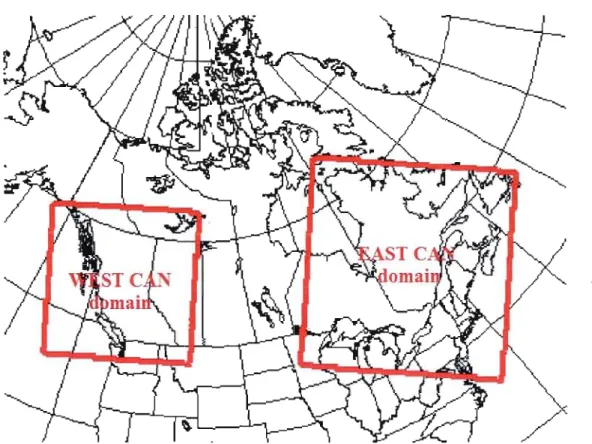
Geographical position of the two CRCM4 simulation domains (WEST CAN and
EAST CAN) used in this study 56
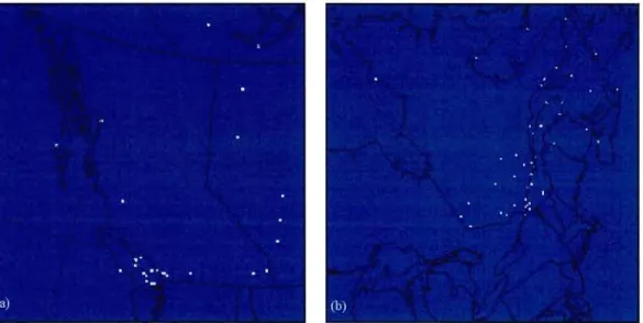
2 Position of the weather stations of the Environment Canada's hourly-precipitation
network on the 15-km grid (in white) over (a) the WEST CAN domain and (b) the EAST CAN domain. Only stations kept for analysis are shown. A total number of 27 stations is used over the WEST CAN domain (a) and a total of 45 stations is used
over the EAST CAN domain (b) 57
3 Mean annual precipitation amount observed (1961-1990) over the WEST CAN
domain with the position and name of the main topographie barri ers (after the Pacifie
Climate Impacts Consortium, PCIC) 58
4 4-year annual mean sea level pressure (magenta contours; hPa), horizontal wind
speed (background ftled contours; km/h) and horizontal wind direction (black
arrows) for the simulations W 15 (a) and W45 (b) 59
5 4-year annual mean total precipitation rate (mm/day) for the simulations W15 (a) and
W45 (b). Panel (c) shows the domain-averaged mean annual cycle of total precipitation. On the bottom left corner of panels (a) and (b) is given the domain
average of the total precipitation rate (mm/day) 59
6 Topography (m) of the simulations W15 (a) and W45 (b) 60
7 4-year annual mean total precipitation rate (mm/day or mm/year) for the simulations
W15 (a) and W45 (b) zoom over a portion of the WEST CAN domain surrounding
the Vancouver and Victoria area 60
8 Top: 4-year annual mean convergence of humidity (mm/day) for the simulations
W15 (a) and W45 (b). Panel (c) depicts the domain-averaged mean annual cycle of
convergence of humidity. Middle: 4-year annual mean evapotranspiration (mm/day)
for the simulations W15 (d) and W45 (e). Panel (f) presents the domain-averaged
mean annual cycle of evapotranspiration. Bottom: 4-year annual mean total
precipitation rate (mm/day) for the simulations W15 (g) and W45 (h). Panel (i)
shows the domain-averaged mean annual cycle of total precipitation. On the bottom left corner of panels (a), (b), (d), (e), (g) and (h) is given the domain average of the
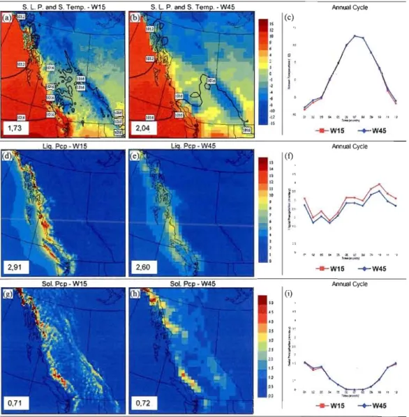
9 Top: 4-year annual mean sea level pressure (black contours; hPa) and screen temperature (oC) for the simulations W15 (a) and W45 (b). Panel (c) shows the domain-averaged mean annual cycle of screen temperature. Middle: 4-year annual mean liquid precipitation rate (mm/day) for the simulations W15 (d) and W45 (e). Panel (f) presents the domain-averaged mean annual cycle of liquid precipitation. Bottom: 4-year an nuai mean solid precipitation rate (mm/day) for the simulations W15 (g) and W45 (h). Panel (i) depicts the domain-averaged mean an nuai cycle of sol id precipitation. On the bottom left corner of panels (a), (b), (d), (e), (g) and (h) is given the domain average of the respective variables 62
10 Top: 4-year annual mean snow water equivalent (mm) for the simulations Wl5 (a) and W45 (b). Panel (c) presents the domain-averaged mean annual cycle of snow water equivalent. Middle: 4-year annual mean runoff (mm/day) for the simulations W15 (d) and W45 (e). Panel (f) shows the domain-averaged mean annual cycle of runoff. Bottom: 4-year mean number of wet days (days/year) for the simulations W15 (g) and W45 (h). Panel (i) presents the domain-averaged mean annual cycle of the number of wet days. On the bottom left corner of panels (a), (b), (d), (e), (g) and (h) is given the domain average of the respective variables 63
Il Mean annual cycle of precipitation (mm/day and mm) for model simulations (W 15 and W45) and observations. The curves represent the mean annual cycle of ail the 27 stations (for observations) or grid points (for model simulations) used in this study
(see section 3.3) 64
12 Observed and simulated (W15 and W45) distributions obtained with a I-h accumulation interval. (a) 4-year mean precipitation frequency (%), (b) 4-year mean number of weather stations (for observations) and grid points (for model), (c) 4-year mean precipitation intensity (mm/h), and (d) 4-year mean cumulative annual precipitation amount (mm). The x-axis represents the Hourly Precipitation Event (HPE) in units of mm/h, with the number on the axis being the threshold of a HPE class. The width of each HPE class is 0.2 mm/ho On each panel, the curves represent the mean distributions of ail the 27 weather stations (for observations) or grid points (for model simulations) used in this study (see section 3.3) 65
13 Observed and simulated (W15 and W45) distributions obtained with a 24-h accumulation interval. (a) 4-year mean precipitation frequency (%), (b) 4-year mean number of weather stations (for observations) and grid points (for model), (c) 4-year mean precipitation intensity (mm/h), and (d) 4-year mean cumulative annual precipitation amount (mm). The x-axis represents the Daily Precipitation Event (DPE) in units of mm/day, with the number on the axis being the threshold of a DPE class. The width of each DPE class is 1 mm/day, except for the two first classes (0 0.2 mm/day and 0.2-1 mm/day). On each panel, the curves represent the mean distributions of ail the 27 weather stations (for observations) or grid points (for model simulations) used in this study (see section 3.3) 66
15
Top: 4-year annual mean convergence of humidity (mm/day) for the simulations E15
(a) and E45 (b). Panel (c) depicts the domain-averaged mean annual cycle of
convergence of humidity. Middle: 4-year annual mean evapotranspiration (mm/day)
for the simulations E15 (d) and E45 (e). Panel
(f)presents the domain-averaged
mean annual cycle of evapotranspiration. Bottom: 4-year annual mean total
precipitation rate (mm/day) for the simulations E15 (g) and E45 (h). Panel (i) shows
the domain-averaged mean annual cycle of total precipitation. On the bottom left
corner of panels (a), (b), (d), (e), (g) and (h) is given the domain average of the
respective variables
:
68
16
Top: 4-year annual mean sea level pressure (black contours; hPa) and screen
temperature
(oC)for the simulations EI5 (a) and E45 (b). Panel (c) shows the
domain-averaged mean annual cycle of screen temperature. Middle: 4-year annual
mean liquid precipitation rate (mm/day) for the simulations E15 (d) and E45 (e).
Panel
(f)presents the domain-averaged mean an nuai cycle of liquid precipitation.
Bottom: 4-year annual mean solid precipitation rate (mm/day) for the simulations
E15 (g) and E45 (h). Panel (i) depicts the domain-averaged mean an nuaI cycle of
solid precipitation. On the bottom left corner of panels (a), (b), (d), (e), (g) and (h) is
given the domain average of the respective variables
69
17
Top: 4-year annual mean snow water equivalent (mm) for the simulations E 15 (a)
and E45 (b). Panel (c) presents the domain-averaged mean annual cycle of snow
water equivalent. Middle: 4-year annual mean runoff (mm/day) for the simulations
El5 (d) and E45 (e). Panel
(f)shows the domain-averaged mean an nuaI cycle of
runoff. Bottom: 4-year mean number ofwet days (days/year) for the simulations E15
(g) and E45 (h). Panel
(i)presents the domain-averaged mean annual cycle of the
number of wet days. On the bottom left corner of panels (a), (b), (d), (e), (g) and (h)
is given the domain average of the respective variables
70
18
Mean annual cycle of precipitation (mm/day and mm) for model simulations (E 15
and E45) and observations. The curves represent the mean annual cycle of ail the 45
stations (for observations) or grid points (for model simulations) used in this study
(see section 3.3)
71
19
Observed and simuJated (E 15 and E45) distributions obtained with a I-h
accumulation interval. (a) 4-year mean precipitation frequency
(%),(b) 4-year mean
number of weather stations (for observations) and grid points (for model), (c) 4-year
mean precipitation intensity (mm/h), and (d) 4-year mean cumulative annual
precipitation amount (mm). The x-axis represents the Hourly Precipitation Event
(HPE) in units of mm/h, with the number on the axis being the threshold of a HPE
class. The width of each HPE class is 0.2 mm/ho On each panel, the curves represent
the mean distributions of ail the 45 weather stations (for observations) or grid points
(for mode] simulations) used in this study (see section 3.3)
72
20
Observed and simulated (E 15 and E45) distributions obtained with a 24-h
accumulation interval. (a) 4-year mean precipitation frequency
(%),(b) 4-year mean
number of weather stations (for observations) and grid points (for model), (c) 4-year
mean precipitation intensity
(mm/h),and (d) 4-year mean cumulative annual
precipitation amount (mm). The x-axis represents the Daily Precipitation Event
(DPE) in units of
mm/day,with the number on the axis being the threshold of a DPE
class. The width of each DPE class is 1
mm/day,except for the two first classes (0
0.2 mm/day
and 0.2-1
mm/day).On each panel, the curves represent the mean
distributions of aIl the 45 weather stations (for observations) or grid points (for model
simulations) used in this study (see section 3.3)
73
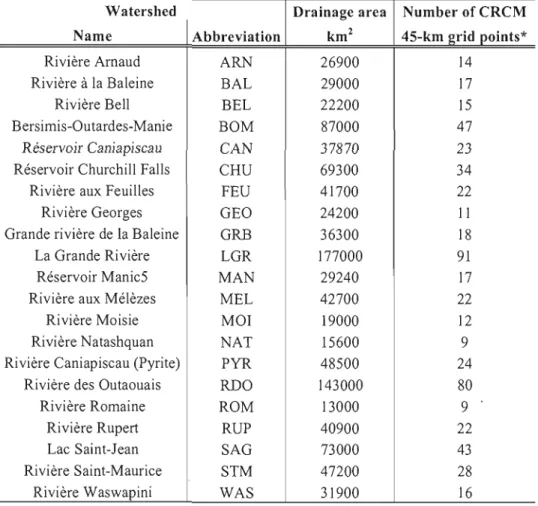
21
Geographical positions and abbreviations of the 21 watersheds of interest on the 45
km CRCM grid. Thanks to the Ouranos Consortium for the computer program used
to create this figure
74
22
4-year annual mean (a) convergence of humidity
(mm/day),(b) evapotranspiration
(mm/day),
(c) total precipitation
(mm/day),(d) runoff
(mm/day)over each of the 21
watersheds of interest. Values for the simulation E15 are in red while values for the
simulation E45 are in bleu. Thanks to the Ouranos Consortium for the computer
program used to create this figure
75
23
4-year annual mean (a) screen temperature
(oC),(b) snow water equivalent (mm), (c)
liquid precipitation
(mm/day),(d) solid precipitation
(mm/day)over each of the 21
watersheds of interest. Values for the simulation E15 are in red while values for the
simulation E45 are in bleu. Thanks to the Ouranos Consortium for the computer
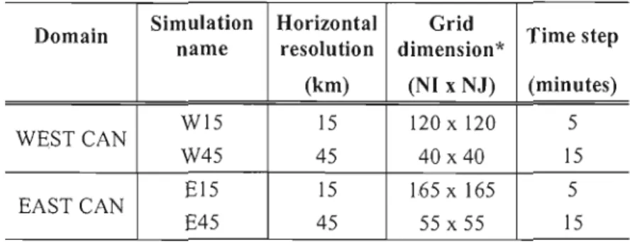
3.1
Main characteristics of the simulations used in this study
53
4.1
Mean annual precipitation amount (mm/year) and mean number of wet days
(days/year) observed at Victoria Int'l Airport and North Vancouver Sonora Dr, and
simulated at the closest grid points to those weather stations
53
4.2
Altitude (m) at the weather stations Victoria Int'I Airport and North Vancouver
Sonora Dr as wel1 as the altitude (m) at the closest grid points and at the most
representative grid points to those stations
54
4.3
List of the 21 watersheds with their respective abbreviated name, drainage area and
APA
BKF
CLASS
CGCM CRCM CRCM4 CRCMD DAI DPE ESCER EASTCAN GCM HPE IPCC ISBA LAM MCG MCGC MRC MRCC MRCC4 NCEP PCIC PE PF PI RCM UQÀM WESTCANAnnual Precipitation Arnount
Bechtold-Kain-Fritsch
Canadian LAnd Surface Scherne
Coupled Global Circulation Model Canadian Regional Climate ModelCanadian Regional Climate Model (4th version) Canadian Regional Modelling and Diagnostics Data Access and Integration
Daily Precipitation Event
Étude et la Simulation du Climat à l'Échelle Régionale Eastern Canada
Global Circulation Model Bourly Precipitation Event
Intergovernmental Panel of Climate Change Interactions Soil-Biosphere-Atmosphere Limited-Area Model
Modèle de Circulation Générale Modèle de Circulation Générale Couplé Modèle Régional du Climat
Modèle Régional Canadien du Climat
Modèle Régional Canadien du Climat (4e version) National Centers for Environmental Prediction Pacifie Climate Impacts Consortium
Precipitation Event Precipitation Frequency Precipitation Intensity Regional Climate Model
Université du Québec à Montréal Western Canada
canadien (EAST CAN). Pour ces deux régions, chaque paire de simulations consiste en une simulation dont la résolution horizontale est de 15 km (vrai à 60° N) et une simulation dont la résolution horizontale est de 45 km (vrai à 60° N). En utilisant ces simulations, cette étude tente de déterminer l'impact de l'augmentation de la résolution horizontale sur le champ de précipitation du modèle. Les résultats montrent que l'augmentation de la résolution horizontale permet d'obtenir une représentation plus réaliste de la topographie dans les simulations à 15 km, puisqu'elles illustrent de plus fines caractéristiques du terrain, tels que d'étroites et profondes vallées ainsi que de hauts, mais petits, complexes montagneux. De plus, notre étude révèle que les simulations à 15 km produisent davantage de convergence d'humidité et d'évapotranspiration, menant ainsi à une augmentation de la précipitation. L'augmentation de la résolution permet à la simulation à 15 km de produire de la neige durant toute l'année au sommet des plus hautes montagnes du domaine WEST CAN. Pour le domaine EAST CAN, la précipitation totale et solide plus grande retrouvée dans la simulation à 15 km mène à un ruissellement supérieur à celui retrouvé dans la simulation à 45 km.
En comparant la précipitation simulée avec la précipitation observée provenant du réseau de stations d'Environnement Canada mesurant la précipitation horaire, on trouve que les simulations à 15 km produisent une distribution de la fréquence des précipitations horaires et une distribution de l'intensité des précipitations plus réaliste. Contrairement aux simulations à 15 km, les simulations à 45 km produisent moins d'événements horaires d'intensité modérée à très forte (3-10 mm/h) que ce qui est observé. Néanmoins, autant les simulations à 15 km que celles à 45 km produisent un biais positif en termes de fréquence et d'intensité des événements horaires de faibles intensités (0,2-3 mm/h). Conséquemment, une trop grande quantité de précipitation est générée annuellement par ce type d'événements, comparativement aux observations. La précipitation simulée est alors généralement plus grande que celle observée. Notre étude révèle également que pour analyser la fréquence et l'intensité de la précipitation,
il
est plus approprié d'utiliser une période d'accumulation d'une heure plutôt qu'une période d'accumulation de 24 heures. En effet, cela nous permet de comprendre plus facilement quels types d'événements le modèle est capable de reproduire et quelle est la contribution (en termes de quantité de précipitation) de chacun de ces événements.vie est possible. De plus, la coexistence simultanée des trois phases de l'eau (vapeur, liquide et solide) fait la particularité de notre planète (Webster, 1994). Sous une de ces trois phases, d'importantes quantités d'eau sont échangées entre les océans, l'atmosphère, le continent (l'eau des sols et l'eau de surface), la cryosphère et la biosphère. Ceci forme le cycle
hydrologique. Ce cycle contrôle le climat à travers plusieurs interactions complexes (Peixoto
and Oort, 1992). Sous l'action du rayonnement solaire, l'eau provenant des océans et des surfaces continentales est introduite dans l'atmosphère par évapotranspiration. Elle est transportée par le vent en phase vapeur, pour ensuite être condensée et stockée dans les
nuages. Elle retombe finalement
à
la surface sous forme de précipitation liquide ou solide.Ceci constitue la branche atmosphérique du cycle hydrologique. Une fois précipitée à la
surface, l'ea!1 peut s'infiltrer dans le sol ou ruisseler (surface ou souterrain), ce qui alimente les cours d'eau et les océans. L'eau demeurée en surface ou absorbée par les plantes est
ensuite évapotranspirée à nouveau et le cycle se poursuit. Ceci constitue la branche terrestre
du cycle hydrologique. Parmi toutes les composantes du cycle hydrologique, la précipitation est probablement celle qui influence les plus nos activités quotidiennes (loisirs, travail, etc.). Il est donc primordial de connaître de quelle façon cette variable météorologique évoluera avec les changements climatiques. Afin de simuler le climat futur, les scientifiques ont
maintenant recours à des modèles climatiques.
Depuis quelques années, plusieurs études ont été menées dans le but d'évaluer la capacité
des modèles climatiques à simuler la précipitation (Mearns et al., 1995; Chen et al., 1996;
Giorgi et Marinucci, 1996; Dai et al., 1999; Gutowski Jr. et al., 2003; Sun et al. 2006). Ces
études ont montré que la plupart des modèles sont capables de reproduire la distribution
spatiale de la précipitation, mais qu'ils ont de la difficulté à bien reproduire d'autres
caractéristiques importantes de cette variable, tel que le cycle diurne, la fréquence et l'intensité. En utilisant la précipitation simulée par 18 Modèles de Circulation Généraux Couplés (MCGC), Sun et al. (2006) ont déterminé que la plupart des modèles surestiment la
fréquence de la précipitation faible (1-10 mm/jour) tout en reproduisant adéquatement
l'intensité de ce type d'événements. Pour les événements de précipitation forte (> 10
mm/jour) toutefois, la pluparts des MCGCs sont capable de reproduire adéquatement la fréquence observée, mais ils en sous-estiment l'intensité. Une autre étude, réalisée par Christensen et al. (1998), a permis de démontrer que les Modèles Régionaux du Climat (MRCs) possèdent des difficultés semblables. En effet, les auteurs établissent que les MRCs
surestiment généralement la fréquence des événements de trace de précipitation
«
0.1mm/jour) et qu'ils sous-estiment la fréquence de la précipitation faible à forte (> 0.1
mm/jour). De plus, d'autres études antérieures ont permis de découvrir que les modèles climatiques produisent typiquement davantage d'événements de faibles intensités par rapport
à ce qui est observé (Meams et al., 1995; Chen et al., 1996; Giorgi et Marinucci, 1996; Dai et
al., 1999; Gutowski Jr. et al., 2003). Les modèles climatiques actuels doivent mieux reproduire la fréquence et l'intensité de la précipitation pour ainsi pouvoir prévoir
adéquatement leur changement en climat futur. Par ailleurs, l'augmentation des gaz à effet de
serre semble entrainer une augmentation de la fréquence des événements de précipitation forte, de même qu'un accroissement de la fréquence des sécheresses. Résultant d'une augmentation de la température et de l'humidité spécifique, une amplification du cycle hydrologique est ainsi prévue (Trenberth, 1999; Trenberth, 2003). Donc, étant donné que ces changements auront un impact important sur l'activité humaine, il est primordial que les
modèles soient très habiles à simuler ces caractéristiques de la précipitation.
De nos jours, l'utilisation d'un MRC à aire limitée au-dessus d'une région d'intérêt est le
principal moyen de simuler les caractéristiques régionales de la précipitation. Les MRCs permettent une représentation plus fine de l'échelle spatiale que les Modèles de Circulation
Généraux (MCGs). Présentement, la plupart des modèles à aire limitée opérationnels ont une
résolution horizontale variant entre 20 et 50 km. Même à ces résolutions, la topographie n'est
pas parfaitement représentée et certains aspects du terrain sont tout de même manquants, ce qui peut avoir un impact significatif sur la simulation des différentes variables
atmosphériques, principalement la précipitation. Bref, même à de telles résolutions
horizontales, les processus de fines échelles (dont la résolution spatiale est supérieure à la
sont une source d'incertitudes dans les simulations climatiques puisqu'ils sont basés sur des approximations et simplifications. D'ailleurs, un effort international est mené dans le but d'améliorer les schémas existant ou bien encore pour en créer de nouveaux afin que les processus de fines échelles soient mieux représentés dans les modèles numériques. Avec une augme,ntation de la résolution horizontale, la représentation des caractéristiques de surface devrait être meilleure, ce qui fait que les modèles devraient mieux résoudre les phénomènes de fines échelles. Certaines études ont été menées dans le passé pour connaître l'impact d'une augmentation de la résolution horizontale sur les champs atmosphériques. Dans leur étude, Christensen et al. (1998) ont analysé le comportement des composantes du cycle hydrologique simulées par un MRC et un MCG. Pour réaliser cette étude, les auteurs ont utilisé une technique de double-pilotage dans laquelle un MRC ayant une résolution horizontale de 19 km était piloté aux frontières par un autre MRC ayant une résolution horizontale de 57 km. Ce dernier MRC était lui piloté aux frontières par un MCGC. L'étude montre qu'en terrain montagneux, la simulation à haute résolution montrait d'importantes améliorations dans la représentation du ruissellement de surface et du couvert de neige. L'étude montre également que la distribution de la précipitation selon différentes classes d'intensités est plus réaliste avec la simulation à haute résolution.
L'objectif de la présente étude est d'évaluer l'impact de l'augmentation de la résolution horizontale sur la précipitation, aussi bien que sur d'autres composantes du cycle hydrologique, simulés avec la quatrième génération du Modèle Régional Canadien du Climat (MRCC4) au-dessus de deux régions climatiques distinctes. Les simulations du MRCC4 sont en fait produites au-dessus de deux don:aines de l'Amérique du Nord: 1) centré sur la province de la Colombie-Britannique (ouest canadien) et 2) centré sur la province du Québec (est canadien). Pour chacune de ces régions, une paire de simulations d'une durée de quatre ans, pilotée aux frontières par les réanalyses NCEP NRA-2 est analysée. Cette paire de simulations consiste en une simulation ayant une résolution horizontale de 15 km, et une simulation ayant une résolution horizontale de 45 km.
Ce mémoire est écrit sous la forme d'un article. La première partie comprend un court résumé des études antérieures portant sur la précipitation simulée par les modèles climatiques
(MRCs et MCGs), un bref descriptif du MRCC et une description de la méthodologie utilisée. La convergence d'humidité, l'évapotranspiration, la précipitation (totale, liquide et
solide), la température à 2 m, l'équivalent en eau de la neige, le ruissellement de surface et le
nombre de jours de précipitation par année constituent les champs météorologiques simulés qui seront étudiés de plus près. La précipitation simulée par le MRCC est également
comparée avec la précipitation horaire observée, tout en portant une attention particulière à la
Michael
Jr. Powers
1,3,Daniel Caya
1,2,3and René Laprise
1,31 Canadian Regional Modelling and Diagnostics (CRCMD) Network, Université du Québec à Montréal
2 Ouranos Consortium C/imate Simulations Team
] Centre pour l'étude et la simulation du climat à l'échelle régionale (ESCER Center)
Septembre 20
IlCorresponding author address:
Michael Jr. Powers
Dép. Sciences de la terre et de l'atmosphère Université du Québec à Montréal (UQAM) 201, President-Kennedy Avenue, 6thfloor Montréal, QC, Canada, H2X 3Y7
performed over two different regions of Canada: 1) western Canada (hereafter WEST CAN) and 2) eastern Canada (hereafter EAST CAN). For both regions, each pair of simulations
consists of one 15-km resolution (true at 600
N) run and one 45-km resolution (true at 60 ON) run. Using these simulations, this study investigates the impact of increasing horizontal resolution on the precipitation field. Results show that increasing horizontal resolution allows a more realistic representation of the topography in the 15-km simulations, by showing smaller scale features such as long and narrow valleys as weil as high and narrow mountains. This investigation also reveals that the l5-km simulations produce more water vapour convergence and more evapotranspiration, which leads to an increase of precipitation in the 15-km simulations. The higher resolution also allows the 15-km simulation to capture sorne of the permanent snow present at the top of the high mountains within the WEST CAN domain. Over the EAST CAN domain, the greater l5-km total and solid precipitation leads to more runoff than within the 45-km simulation.
When comparing simulated precipitation with observed precipitation from Environment Canada's hourly precipitation network, it is found that the 15-km simulations depict more realistic hourly precipitation frequency (hereafter PF) and precipitation intensity (hereafter PI) distributions than the 45-kmsimulations. Contrary to the 15-km simulations, the 45-km simulations produce less moderate-to-very-heavy (3-10 mm/h) hourly precipitation events (hereafter HPE) than those observed. Nevertheless, both simulations produce a positive bias in the frequency and intensity of light HPE (0.2-3 mm/h), which leads to an annual precipitation amount too large, in comparison with observations, generated by those events. Thus, the simulated precipitation tends to be greater than the observed precipitation. Our investigation also revealed that using an hourly accumulation interval to analyse the PF and PI was more appropriate than using a daily accumulation interval in understanding which events the model is able to reproduce and what the contribution (in precipitation amount) of each type of event is.
1 Introduction
Over the recent years, many studies have been carried out to see how weil climate models
simulate precipitation (Chen et al. 1996, Dai et al. 1999, Gutowski Jr. et al. 2003, Sun et al.
2006). These studies showed that most models can usually reproduce the spatial distribution and climatological mean of precipitation, but tend to fail in reproducing someother important features of this atmospheric variable, such as the diurnal cycle, the frequency and the intensity. Using 18 different Coupled Global Circulation Models (CGCMs), Sun et al. (2006) found out that most models overestimate the frequency of light precipitation (1-10 mm/day)
but reproduce adequately the intensity of those events. For heavy precipitation (> 10
mm/day), their study revealed that most CGCMs are able to reproduce quite properly the observed frequency, but underestimate the intensity of such events. Another study realised by Christensen et al. (1998) showed that Regional Climate Models (RCMs) have similar difficulties. Indeed, the authors found that RCMs tend to underestimate the frequency of trace
precipitation events
«
0.1 mm/day) while they overestimate the frequency of low-to-heavyprecipitation events (> 0.1 mm/day). Moreover, other past studies discovered that climate
models produce typically more light precipitation events than what is observed (Mearns et al. 1995, Chen et al. 1996, Giorgi et Marinucci 1996, Dai et al. 1999, Gutowski Jr. et al. 2003). Thus, the frequency and intensity of precipitation need to be weIl reproduced by climate models to adequately project their change in future climate. Besides, the frequency of heavy precipitation events is expected to increase, as weil as the frequency of droughts. An enhancement of the hydrological cycle is also expected resulting from the increase in air temperature and specifie humidity (Trenberth 1999, Trenberth 2003). Since these changes will have significant impacts on human activities, there is a real need for models to have very good skills in simulating these precipitation features.
Nowadays, the use of a limited-area (LAM) RCM over an area of interest is the principal way to simulate regional characteristics of precipitation. RCMs allow a finer representation of the spatial scale than a GCM. Currently, most operation al LAMs have a horizontal resolution of about 20 to 50 lan. Even at these resolutions, the surface topography is not
perfectly represented and sorne aspects of the terrain are still missed, which can have significant impacts in simulating properly the different atmospheric variables, especially precipitation. Therefore, even at these horizontal resolutions, small-scale processes (whose spatial scales are smaller than the RCM resolution) still need to be parameterized. The parameterization schemes are sources of uncertainties in simulations since they are based on many approximations and assumptions. As a result, an important work is made intemationally to improve the existing schemes or to create new ones to better represent the small-scale processes within models. With an increase in horizontal resolution, the model should better resolve more small-scale features resulting from an improved representation of the land surface characteristics. Studies have been carried out in the past to investigate the influence of increased horizontal resolution on the simulated atmospheric fields. Christensen et al. (1998) analyzed the behavior of the components of the hydrological cycle as simulated by an RCM and a GCM. In a double-nesting approach over Scandinavia, the authors used a 19-km horizontal resolution RCM nested into a 57-km horizontal resolution RCM simulation, which in turn was driven by a Cou pied GCM (CGCM). They found that in mountainous regions, the high-resolution simulation showed improvements in the representation of runoff and snow coyer. They also found that the distribution of precipitation on different intensity classes was more realistic when simulated by the high-resolution simulation.
The obj ective of this study is to investigate the impact of increasing horizontal resolution on precipitation as weil as on other components of the hydrological cycle within the fourth generation of the Canadian Regional Climate Model (CRCM4) over two very distinct climate regions. CRCM4 simulations are performed over two different domains of North America: 1) centered over the province of British-Colombia (Western Canada), and 2) centered over the province of Québec (Eastern Canada). For each region, a pair of 4-year simulations forced at their boundary by the reanalysis NCEP NRA-2 is analyzed. This pair of simulations consists in one 15-km horizontal resolution run to be compared to a one 45-km horizontal resolution run. Precipitation, screen temperature and other components of the hydrological cycle
(convergence of humidity, evapotranspiration, liquid and solid precipitation, lUnoff, snow
model precipitation outputs are then compared to hourly-precipitation observations. Throughout this study, an emphasis is put on the frequency and intensity of precipitation.
The text is organised as follow: section 2 gives a brief description of the model used. Section 3 presents the experiments and methodology, with a description of the model simulations and observations employed, as weil as the model-observation comparison methodology. Section 4 presents the results obtained through this study. Finally, section 5 gives a summary and concludes.
2
Model Description
Originally developed at the Université du Québec à Montréal (UQAM), the CRCM is a
limited-area model (LAM) driven at its boundaries by the large-scale circulation from either reanalyses or global climate models. The mo"del integrates the fully elastic nonhydrostatic Euler equations, which are solved by an off-centered semi-implicit and semi-Lagragian numerical algorithm (Caya 1996, Laprise et al. 1998, Caya and Laprise 1999). The CRCM horizontal grid is uniform in a polar stereographie projection and its vertical resolution is variable using the scaled terrain-following Gal-Chen coordinate. In the CRCM, the precipitation results from two processes: the large-scale precipitation (resolved) and the small-scale precipitation (parameterized). The large-scale precipitation arises from a simple supersaturation-based condensation scheme while the small-scale precipitation comes from the Bechtold-Kain-Fritsch (BKF) mass flux scheme (Bechtold et al. 2001; Paquin et al.
2002), adapted to the CRCM resolution. ln this study, we use the fourth generation of the
CRCM (CRCM4), which is the operational version of the model developed and used by the Ouranos Consortium Climate Simulations Team. This version of the model includes the version 2.7 of the Canadian LAnd Surface Scheme, CLASS2.7 (Verseghy 1991; Verseghy et al. 1993). The CRCM4 also allows spectral nudging, which is a method in which the model's large scales are partially or completely replaced by the nested long-waves at every time step (see Storch et al. 1999, Riette and Caya 2002, Alexandru et al. 2009). More informations on the CRCM4 can be found in Music and Caya (2008).
3 Experiments and methodology
3.1 Description of the model simulations
In this study, CRCM4 simulations are performed over two different regions of Canada: western Canada (hereafter WEST CAN) and eastern Canada (hereafter EAST CAN). These two domains (see Fig. 1 for geographical position of the domains) have been chosen for their different climate regime and physiography. The WEST CAN domain is a mountainous region (with surnrnits reaching more than 4000 m) along the Pacifie coast. The WEST CAN domain is almost always under the influence of a humid air flow coming from the Pacifie Ocean toward the topographie barrier, which then represents an important factor in the formation of precipitation. In comparison to the WEST CAN domain, the EAST CAN domain has a much flatter terrain (with the highest mountain slightly above 1000 m) and the topography do es not play as much an important role in the formation of precipitation as it does in western Canada. However, the domain is located in a Storm-Track corridor and many low-pressure systems from different origins cross the province of Québec. Those low pressure systems generally come from the Rocky Mountains, the Gulf of Mexico or the East Coast of United-States (Zishka and Smith, 1980).
For both regions (WEST CAN and EAST CAN), two 4-year-Iong (December 2001 to November 2005) simulations forced at their boundary by the NCEP NRA-2 reanalysis are
used (Table 3.1). These two simulations consist in one 15-km-resolution (true at 600 N) run
with a 5-minute time step and one 45-km-resolution (true at 60 ON) run with a 15-minute time step. Note that the simulations are originally performed from January 1999 to November 2005, from which a spin-up of 35 months has been taken off. AIso, the spectral nudging was not applied in these runs because of the small size of the domains.
3.2 Description of the water cycle components analysis
The hydrological cycle controls and regulates climate in a fundamental way through many complex interactions (Peixoto and Oort, 1992). Therefore, our analysis in this study is not limited to the total precipitation, but also includes the main components of the hydrological cycle (convergence of humidity, evapotranspiration, liquid and solid precipitation and runoft) as simulated by the CRCM. Along with these components, we also analyse the surface temperature, snow water equivalent and number of wet days. For bath domains, we qualitatively compare the 4-year annual mean of these 15-km CRCM-simulated variables to that of the 45-km CRCM-simulated variables. We also contrast the CRCM 15 km and 45-km domain averages of each variable, as well as their domain-averaged mean annual cycle.
As shown in Music and Caya (2007), the water cycle can be separated into two branches: atmospheric and terrestrial. Applying the law of water mass conservation in a given control volume leads to the water budget equation. The water budget equation for an atmospheric colurnn (per unit area) can be written as
aw
- = - V
at
eQ-p+E
(1)H
where
W
(kg m·2) is the precipitable water in the atmosphere, which represents the amountof water that would precipitate if ail the water vapor in a column of the atmosphere were
condensed,
E
(kg m'2 S·I) is evapotranspiration, andP
(kg m'2 S·I) is precipitation. Theoperator
V
H is the horizontal divergence andQ
is the vertically integrated horizontal watervapor flux:
Q=
rU"
qy dp (2)Ps g
where
q,
Y, andg
represent respectively the specifie humidity, the horizontal velocityvector, and the gravitational acceleration. The lower limit in the integral (p
J
is the surfaceIn Equation l, the term -
V
rI •Q
is the horizontal convergence water vapor flux, C(hereafter convergence of humidity). Replacing the convergence of humidity term by Cinto Equation 1 leads to
aw
-+P=C+E
(3)at
Taking time and spatial averages of the atmospheric water budget equation (3) over a multiyear period and over the whole domain leads to
[P] =
[C]
+
[E]
(4)where
X
is the time average of the componentX, and
[X]
is the domain average. Theterm
[aW / at]
can be neglected because it tends to zero when averaged over a long period oftime (Music and Caya, 2007). When considering the 4-year annual mean domain average of
these components, Equation 4 can be used. Precipitation occurs when the available water vapor condenses and falls on the ground. Thus, Equation 4 establishes that the water vapor available to generate precipitation can come from two different sources: convergence of humidity or evapotranspiration.
As fully explained in Music and Caya (2007), applying the water conservation law to a
land colurnn and then taking time and spatial averages of the terrestrial water budget equation over a multiyear period and over the whole domain leads to
[R] =
[P]-[E]
(5)where R (kg m'2 S·I) is the total runoff. Equation 5 can also be used when considering the 4
year annual mean domain average of these components. Equation 5 then establishes that the runoff is equal to the amount of water that precipitates minus the amount that goes back into the atmosphere through evapotranspiration.
3.3 Description of the observations
The observational data used in this study consist in the Environment Canada's hourly precipitation network of weather stations (DAI Catalogue, 2009). Most of these stations are
automatic and measure the hourly accumulation of precipitation with ~ither a Fisher Porter or
a tipping-bucket rain gauge. The threshold of these instruments may vary from one station to another with ranges between 0.1 mm/h and 0.2 mm/h. For this reason, we have chosen 0.2 mm/h has the corn mon threshold for ail the stations and then, any amount inferior to this is brought back 0 mm/h. For the present study, we only used the stations that are located into our two domains of interest, and we rejected the stations that had more than 50% of missing values through the 4-year period. This criterion left us with a total of 27 stations for the WEST CAN domain and of 45 stations for the EAST CAN domain (Fig. 2).
3.4 Model-observation comparison methodology
Over both domains, the simulated precipitation was compared to the observed precipitation fol1owing this procedure. First, we find the closest CRCM4 grid point (center of the grid-box at 15-km and 45-km) to each station, resulting in the same number of model grid points than of stations. The fact of choosing the closest CRCM grid point to a station has sorne consequences worth mentioning here: 1) the closest grid point may not necessarily be a land point in the model, and 2) sorne grid points may contain more than one station, meaning that one grid point may be the closest to two (or more) different stations. For the WEST CAN domain, the simulation W 15 has 21 grid points out of 27 being considered as land while this number is 26 for the simulation W45. For the EAST CAN domain, the simulation EI5 has 36 grid points out of 45 being considered as land while the simulation E45 has 32. In the 15-km simulations, the number of different grid points always equals the number of stations meaning that there is no more than one station falling in a grid point. However, in the 45-km simulations, sorne grid points contain two stations. In fact, the number of different grid points is 23 for the simulation W45 and 42 for the simulation E45.
Once the closest grid point to the station is found (for each domain), we then have three different hourly-precipitation time series (observed, CRCM4 15-km and CRCM4 45-km) that can be compared. While comparing these three time series, if there is a missing value in the observed time series, the corresponding simulated value is discarded. Then, we assign a value of 0 mm/h to any simulated precipitation values being below the instrument's threshold (0.2 mm/h). Next, using the hourly time series, we build the daily time series by accumulating precipitation over a 24-hour period. With these 4-year long time series, we calculate the following climatological 4-year means for each location: the annual cycle, the precipitation frequency per intensity interval, the precipitation intensity per intensity interval, and the cumulative annual precipitation amount per intensity interval. These variables have been chosen for the following reasons. First, as mentioned in the introduction, the frequency and intensity of precipitation is expected to change in future climate (Trenberth 1999, Trenberth 2003). Second, there is a need to find out if the model can correctly reproduce both the mean observed precipitation frequency and the mean observed precipitation intensity. Indeed, a model might simulate properly the mean precipitation rate over a region but this could come
from a wrong combination of frequency and intensity. Plus, dividing precipitation in intensity
intervals allows a better understanding of what kind of events the model has the best skill to reproduce.
4 Results and Discussions
4.1 WEST CAN domain
4.1.1 Analysis of precipitation
As mentioned in section 3.1, topography plays a key role in the formation of precipitation over western Canada (WEST CAN domain). In winter, a flow of moist air is brought into the continent by a climatological surface pressure system known as the Aleutian low (located in middle north Pacifie; Ahrens 2003). During summer, the Pacifie high replaces the Aleutian low (Ahrens 2003), which reduces the transport of moist air into the region (especially in southern British Columbia, Canada) and then reduces precipitation. However, there is on average an almost constant southwesterly flow (at the surface) of hum id air coming from the Pacifie Ocean. Once brought over the continent, this moist air encounters a first topographie barrier along the Coastal Range. When reaching the barrier, this hum id air is forced to rise, condense, and eventually to precipitate on the upwind side of the mountains, resulting in a strong band of precipitation maximum along the Pacifie Coast as it can be seen in Figure 3. On the downwind side of this first series of mountains, the air subsides and creates a drier region between the Coast and the Rocky Mountains. Then, the atmospheric circulation meets a higher topographie barrier (the Rocky Mountains) and again, the air rises, condenses and precipitates on the upwind side of the mountains resulting in a second band of precipitation maximum along the boundary of British-Columbia and Alberta (Fig. 3). This second band of maximum is less intense than the first one since the air has already lost some of its humidity through the journey. East of the Rocky Mountains, dry conditions prevail. Both simulations W 15 and W45 reproduce the southwesterly flow over the region as can be se en in Figure 4, which shows the mean sea level pressure as weil as the horizontal wind speed and direction. Moreover, both simulations capture weil the climatological pattern of precipitation (Fig. 5a b). Of course, differences exist between the two simulations as the l5-km total precipitation rate tends to be overall larger than the 45-km precipitation (3.63 nunlday vs 3.32 nunlday). The two bands of precipitation maximum are defined better in the l5-km run than in the 45
km run. The annual cycle shows that most of the precipitation falls during the cold months (October to March; Fig. Sc) which is in line with the observed climatology.
When looking at RCM simulations, it is important to keep in mind that the ability of the model to reproduce the observed climatological pattern is greatly influenced by its own
topography. The model topography is sensitive to the horizontal resolution as it can be seen on Figure 6 where the 45-km and the 15-km topographies are shown. ln the 15-km simulation, the "true" topography is averaged over an are a of 225 km2 compared to an area of 2025 km2 in the 45-km simulation. This means that less topographic details (mountains, hills and valleys) are lost through the process of averaging in the l5-km simulation than in the 45
km simulation (Fig. 6). This leads to a more realistic topography in the 15-km simulation than in the 45-km simulation.
For example, the CRCM 15KM topography (Fig. 6a) shows peaks in northern Washington state (USA) ranging between 1000 m and 1400 m, in the Olympic National Park (with its highest point being Mount Olympus at 2500 m high in reality). However, the CRCM
45KM topography (Fig. 6b) shows a much smaller peak at about 300 m high. The presence of the Olympie National Park Mountains plays an important role on the climate of the surrounding region and the differences between the 15-km and the 45-km topography results in significant differences on the precipitation fleld over the region. The persistent southwesterly flow of humid air meets the mountains and creates abundant precipitation Southwest of the park and drier conditions northeast of it. Located on the leeside of these
mountains, Victoria Int'l Airport (BC, Canada) receives 783 mm of precipitation per year in average and precipitation occurs1 138 days/yea/ (Table 4.1). Only 150 km northeast of
Victoria, the city of Vancouver (BC, Canada) experiences a much wetter climate since it is located on the upwind side of the Coastal Range. The annual precipitation amount observed
1 In this study, whenever we are referring to the number of days with precipitation (also called number
ofwet days), we are referring to the number of days with at least 0.2 mm of precipitation.
2 Based on the Environment Canada's hourly-precipitation network of weather stations used in this
at N Olth Vancouver Sonora Dr is 1975 mm and the number of wet days is 163 days/year (Table 4.1). North Vancouver Sonora Dr receives about twice the amount received in Victoria and there is 20% more rainy days in Vancouver than in Victoria.
The amount of simulated precipitation at the closest grid point of Victoria Int'I Airport in the CRCM l5KM is 1264 mmlyear and it precipitates 166 days/year (Table 4.1). The 45KM simulation generates 1409 mmlyear of precipitation over 198 days/year (Table 4.1). For the Vancouver area, both simulations' topography depicts the Coastal Range even though there are more details at 15-km that at 45-km. As a result, the two simulations generate comparable, but higher than observed, values of annual precipitation at the closest grid point of North Vancouver Sonora Dr. The 15-km simulation generates an annual precipitation amount of 2865 mm and precipitation occurs J75 days/year (Table 4.1). The 45-km simulation produces 2516 mm/year of precipitation and it happens 212 days/year (Table 4. J). The precipitation amount ratio VancouverNictoria is 2.5 in the observations while it is 2.3 for the 15-km simulation and 1.8 for the 45-km simulation. In other words, both simulations reproduce a drier climate for Victoria than for Vancouver and both of them agree that precipitation falls more often over Vancouver than Victoria like in the observations. However, within the 45-km simulation, the difference in precipitation amount between Victoria and Vancouver is somehow incorrect. The 45-km annual precipitation amount for Vancouver is less than twice the amount for Victoria. However, the 15-km annual precipitation amount for Vancouver is about twice the amount for Victoria, which is more in agreement with observations (Table 4.1).
The incorrect precipitation ratio between Victoria and Vancouver highlights an important characteristic of the 45-km precipitation resulting from the weaker precipitation gradient in the W45 simulation than in the WJ5 simulation (Fig. 7). The 45-km precipitation (Fig. 7b) is almost uniform between the Olympie National Park and Victoria, which are about 150 km apart. To the northeast of Victoria, the precipitation in the 45-km simulations starts to gradually increase in direction of Vancouver. In the l5-km simulation (Fig. 7a) however, the
3 Based on the Erivironment Canada 's hourly-precipitation network of weather stations used in this
Southwest-Northeast precipitation gradient in the area is stronger than in the 45-km simulation. In fact, the 15-1<m precipitation captures clearly the rilin-shadow area between the Olympie National Park and Vancouver where Victoria is located.
The latter aspects allow us to understand that the choice of grid point used for comparison with the weather stations might affect the subsequent results. In order to compare model data with observations, we use in this study the closest grid point to the weather station (see section 3.3). However, this does not mean that the closest grid poirt is the most representative grid point to the weather station. What we mean by most representative grid point is a grid point whose surrounding topography is similar to the real topography around the weather station. For example, if a weather station is located at the bottom of a deep valley, the most representative grid point to that weather station should also be located at the bottom of a valley. Because of horizontal resolution though, the valley in the model may not be as deep as in reality or the model valley cou Id be shifted from the real location of the valley, which mày make the closest grid point not the most representative one. With the example of Victoria and Vancouver mentioned above, it turns out that the closest grid point of Victoria Int'l Airport is also the most representative one for both simulations. However, the closest grid point of North Vancouver Sonora Dr is not the most representative grid point for both simulations. Indeed, for the two simulations the closest grid point is in the slope of the mountain (Coastal Range) meaning that the altitude of the closest grid point is too high compared to the altitude of the weather station (Table 4.2) and located in a location with more precipitation (the upslope region). The most representative grid point of North Vancouver Sonora Dr was picked within a one grid point radius of the closest grid point (for both simulations) and is located at the bottom of the mountain (Table 4.2). Using the most representative grid point instead of the closest grid point doest not change the main conclusions mentioned earlier, but it does have an effect. For instance, with the most representative grid point, the 15-km ratio between the Vancouver and Victoria annual precipitation amount is now of 2.5 which is equal to the observed ratio. On the other hand, the 45-km run shows a ratio of 1.3 which is even further away from observations than it was with the closest grid point (Table 4.1). This shows that because the model tries to reproduce a regional climate on a three-dimension grid with finite resolution (horizontal and vertical), the
results are sensitive to the grid point used for comparison. To simplify the comparison between model and observations though, we will use the closest grid point to the weather station asexplained in section 3.3.
4.1.2 Analysis of the water cycle components
The previous results show that the more realistic topography found ,in the 15-km simulation seems to lead to a better spatial distribution of precipitation, especially in valleys or on the lee side of mountains. On the other hand, the simulation W 15 produces globally more precipitation than the simulation W45. Why and how is this humidity generated in the simulations? To answer these questions, we analyzed the contribution of the different components of the hydrological cycle to the total precipitation. We find that both simulations show convergence of humidity on the upwind side of mountains or hills, while on the downwind side of mountains divergence occurs (Fig. 8a-b). The Pacifie Coast has the highest values of convergence of humidity of the entire domain. Over that area, the 15-km convergence of humidity varies from 6 to 12 mm/day (Fig. 8a) while the 45-km convergence of humidity ranges between 6 and 10 mm/day (Fig. 8b). A second less intense maximum of convergence of humidity can also be identified west of the Continental Divide, where the 15 km convergence of humidity is also greater than the 45-km one. Over those regions, most of the total precipitation cornes from convergence while elsewhere on the domain, convergence and evapotranspiration (Fig. 8d-e) respectively provide about half the humidity needed to generate precipitation. Also, both runs agree that evaporation is maximal over the ocean. Between the two topographie barriers and over the prairies, large evapotranspiration rates can also be found. The lowest values of evapotranspiration appear over mountains (Fig. 8d-e). As a result, the simulations W 15 and W 45 both reproduce the two observed bands of precipitation maximum (see Fig. 3) west of the Coastal Range and west of the Rocky Mountains (Fig. 8g-h).
Because the simulation WJ5 produces globally more convergence of humidity and evapotranspiration than the simulation W45, the J5-km total precipitation (Fig. 8g) is larger
than the 45-km total precipitation (Fig. Sh). This latter fact is especially true along the Coastal Range since the 15-km precipitation ranges between 9 to 15 nun/day while the 45-km precipitation ranges between 5 to 10 nun/day. It is also found that the two simulations agree that the highest convergence of humidity is found from November to March (Fig. Sc), which corresponds the wettest period of the year (Fig. Si). In fact, during the winter, most precipitation comes from convergence of humidity brought by many of the low pressure systems coming from the Pacific Ocean. During summer though, about two thirds of the precipitation comes from evapotranspiration (Fig. Sf). However, the minimum of precipitation is reached during the warm season. Being the warrnest period of the year (Fig. 9c), summer time enhances the conversion of evapotranspiration into convective precipitation. Globally, the simulation W 15 is cooler of about 0.3°C than the simulation W45 (Fig. 9a-c). However, it seems that 15-km surface temperature is lower than the 45-km surface temperature during the cold months of the year (November to March; Fig. 9c). AIso, the 15-km simulation is cooler than the 45-km simulation over the northern section of the WEST CAN domain (Yukon and North-West Territories) as weil as over the mountainous regions (Coastal Range, Rocky Mountains and Olympic National Park; Fig. 9a-b). The mean an nuai cycle of surface temperature (Fig. 9c) also reveals that both simulations agree that the surface temperature remains above freezing from April to October. As a result, almost ail of the total precipitation falls as liquid during those months (Fig. 9f). In fact, over the WEST CAN domain most of the total precipitation falls in its liquid forrn. As it can be seen in Figure 9d-f, liquid precipitation contributes respectively to SO% and 78% of the total precipitation within the 15-km and 45-km simulations. Moreover, the 15-km liquid precipitation is greater by about 0.3 mm/da y than the 45-km liquid precipitation, and especially on the upwind side of the Coastal Range (Fig. 9d-e). From December to March, some of the precipitation falls as solid form (Fig. 9i) and both simulations agree that most of that solid precipitation falls over the Coastal Range and over the Rocky Mountains (Fig. 9g-h). Over those areas, the 15-km solid precipitation is greater than the 45-km solid precipitation while over the Alberta prairies the opposite is seen. This leads to a 15-km simulation that produces globally about 0.01 mm/day less solid precipitation than does the 45-km simulation. Since sol id prec.ipitation represents only about 20% of the total precipitation, the 15-km total precipitation remains higher than the 45-km total precipitation.
In addition to solid precipitation, it is also interesting to look at the water equivalent of snow on the ground. The two simulations agree that the snow water equivalent is maximal over the northern section of the domain and over the mountains, with values above 200 mm (Fig. 1Oa-b). This makes sense since we have seen earlier that those regions are the ones receiving the more snow (Fig. 9g-i). Over those regions though, the 15-km snow water equivalent is greater than the 45-km one (Fig. 10a-b). Over the Alberta prairies, the lower 15 km solid precipitation leads to a lower snow water equivalent (especially over northem Alberta), compared with the 45-km snow water equivalent. As a result, the domain average of snow water equivalent is superior within the simulation W 15 than within the simulation W45. On a yearly basis, it is noticeable that the amount of snow water equivalent produced by both simulations is of about 200 min at the end of the win ter (Fig. 1Oc). The 15-km simulation snow water equivalent remains slightly greater than the 45-km one during spring and summer (Fig. 1Oc). This can be explained by the following. Because the 15-km simulation is cooler than the 45-km simulation, snow takes slightly more time to melt in the higher resolution simulation, which explains the difference in snow water equivalent during spring. Moreover, because of the finer horizontal resolution, the 15-1<m run is able to simulate sorne of the permanent snow present at the top of the highest mountains, which keeps the 15-km snow water equivalent slightly above 0 mm during the summer months (Fig. 10c). The latter fact explains why the snow water equivalent is globally greater within the 15-km run than within the 45-km run even though the 15-km solid precipitation is inferior to the 45-km solid precipitation. Since the maximum of runoff is directly linked to the melting of snow and that the solid precipitation is liule bit inferior at 15 km than at 45 km, the maximum of runoff (in April) is lower in the simulation W 15 (Fig. 10f). Over the entire domain, the 15-1<m runof[ is inferior to the 45-1<m runoff, with a respective domain-averaged nmoff of 1.63 mm/day and 1.79 mm/day (Fig. 10d-e). However, both simulations agree that there is more runoff along the Pacific coast associated to the region with the largest precipitation. Moreover, we have seen that the evapotranspiration is superior for the 15-km simulation than for the 45-km one over most of the domain and especially during the warm months (Fig. 3d-f). Therefore, more surface water can be evaporated which also reduce the runof[ in the 15-km simulation with respect to that at 45-km.
In summary, the 15-km simulation produces more precipitation than the 45-km simulation, mostly resulting from the larger convergence of humidity in the 15-km simulation than in the 45-km simulation, especially along the Pacifie Coast. The greater 15-km convergence of humidity found along the coast is explainable by higher 15-km topography over the area (see Fig. 6). Furthermore, figure 9a-b reveals that both simulations reproduce a low pressure system over the Pacifie Ocean. Within the simulation W 15, this low-pressure system generates more than 350 wet days per year, which is about 25 more days than what
the simulation W 45 generates (Fig. 10g-h). In other words, it rains more often in the l5-km
run than in the 45-km run over the Pacifie Ocean. Thus, more humidity (coming from this low) can be transported towards the coast, which is another reason why the convergence of humidity along the coast is greater within the 15-km simulation than within the 45-km simulation. Over the continent, both simulations agree that the number of wet days is greatly correlated with the topographie features: 1) precipitation oCcurs more often on the upwind side of topography, and 2) precipitation is less frequent within the val1eys and on the lee side of mountains (Fig. 10g-h). Because of a more realistic topography, this variable is better defined within the 15-km simulation. In fact, the number of wet days west of mountains and hills is greater in the simulation W 15 than in the simulation W45 (Fig. 10g-h). On the lee side of mountains and hills, the number of wet days seems lower within the l5-km run than within the 45-km run (Fig. 10g-h). When looking globally, it seems that the number of wet da ys is lower at 15-km than it is at 45-km, which can be seen with the domain average of this variable (Fig. 10g-h) as weil as with the annual cycle (Fig. lOi).