Equilibrium transition study for a hybrid MAV

This is an author-deposited version published in:

http://oatao.univ-toulouse.fr/

Eprints ID: 5298

To link to this article: DOI:10.1260/1756-8293.3.4.229

URL: http://dx.doi.org/10.1260/1756-8293.3.4.229

To cite this version:

Itasse, Maxime and Moschetta, Jean-Marc and

Ameho, Yann and Carr, Ryan Equilibrium transition study for a hybrid

MAV. (2011) International Journal of Micro Air Vehicles, 3 (4). pp.

229-246. ISSN 1756-8293

O

pen

A

rchive

T

oulouse

A

rchive

O

uverte (

OATAO

)

OATAO is an open access repository that collects the work of Toulouse researchers and

makes it freely available over the web where possible.

Any correspondence concerning this service should be sent to the repository

administrator: staff-oatao@inp-toulouse.fr

Equilibrium Transition Study for a

Hybrid MAV

Maxime Itasse and Jean-Marc Moschetta

Institut Supérieur de l’Aéronautique et de l’Espace, University of Toulouse, France

Yann Ameho and Ryan Carr

ONERA, Toulouse, France

ABSTRACT

Wind tunnel testing was performed on a VTOL aircraft in order to characterize longitudinal flight behavior during an equilibrium transition between vertical and horizontal flight modes. Trim values for airspeed, pitch, motor speed and elevator position were determined. Data was collected by independently varying the trim parameters, and stability and control derivatives were identified as functions of the trim pitch angle. A linear fractional representation model was then proposed, along with several methods to improve longitudinal control of the aircraft.

1. INTRODUCTION

Modern urban reconnaissance missions dictate the need for a Micro Air Vehicle (MAV) platform capable of performing a complex mission: rapid and efficient ingress to a target location followed by slow loiter for quality image capture. This mission must be performed despite the presence of typical urban obstacles, possible lack of GPS, and erratic wind-gusting. This may be achieved using a tilt-body fixed-wing vehicle which combines the speed, range, and gust-hardiness of a fixed wing with the loiter and precision capability of a rotorcraft vehicle.

The MAVion, shown in Figure 1, has been created for this purpose. It combines a fixed-wing airframe with tandem counter-rotating rotors without resorting to a hollow shaft system as in the case of a coaxial rotor in tractor position. The direction of motor rotation has been chosen to counter wing tip vortices. Also, a tandem-rotor configuration has the advantage of providing an extra degree of freedom to control the vehicle along the yaw axis. From an aerodynamic perspective, it also allows for a larger wing area within the propeller slipstream, yielding higher aerodynamic flap efficiency and a better aerodynamic performance due to a higher aspect ratio.

At the 2009 International MAV competition held in Pensacola, Florida, a team of students from l’Institut Supérieur de l’Aéronautique et de l’Espace (ISAE) demonstrated the horizontal flight capabilities of the MAVion in the outdoor navigation competition. At the 2010 meeting in Braunshweig Germany a vertical version of the aircraft was flown in the indoor competition. Development of the MAVion has continued and the aircraft is now capable of performing fully autonomous transitions between vertical and horizontal flight modes. A wheeled hybrid version of the aircraft has also been developed to enable the MAVion to roll along the ground, walls, or ceilings, increasing its usefulness in indoor settings [1, 2].

There are many ways to transition between horizontal and vertical flight modes [3]. The intent of the current study is to explore equilibrium transition, defined here as maintaining the steady state forces and moments near to zero. This results in an energy efficient change between flight modes with no gain or loss of altitude. Wind tunnel tests were performed to determine the throttle setting, the elevator deflection and the angle of attack for a given velocity during an equilibrium transition.

2. EXPERIMENTAL SETUP AND PROCEDURE 2.1. Experimental Apparatus

Experimental studies on MAVs necessitate a low Reynolds number wind tunnel with the capability of supplying a stable and uniform flow at wind speeds ranging from 2 to 25 m/s. The SabRe wind tunnel located at ISAE has been designed for this purpose [4]. As shown in Figure 2, SabRe is a closed-loop wind tunnel.

The test section is 2400 mm long with a square cross-sectional area of 1200 × 800 mm with a contraction ratio of 9. In order to produce a stable and uniform flow a pitch controlled fan was implemented along with a series of honeycomb grids and screens to split and damp vertical structure. By changing the fan speed and the pitch angle, turbulence intensity can be optimized. For velocities ranging from 2 to 15 m.s−1, typical for a VTOL MAV, the turbulence intensity was found to be lower than 0.1%.

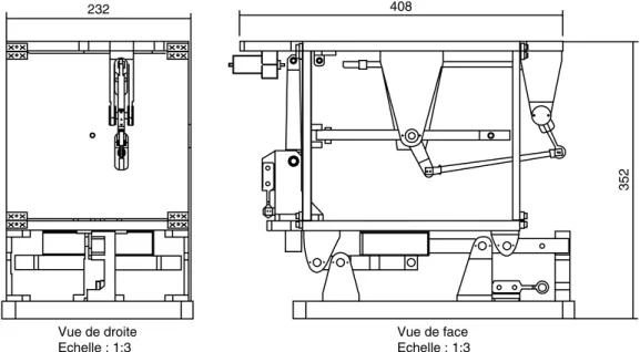
A new 3-component aerodynamic balance devoted to MAV studies was used to measure lift, drag and pitching moment. The balance depicted in Figure 3 was designed to enable measurements at angles of attack between 0 and 90°. Two identical load cells were mounted on the parallelogram balance, giving uncoupled measurements of lift and drag.

The model is attached to the balance by three struts. The two forward supports are fixed at 10.5 cm from the leading edge while the rear, attached above the trailing edge, is raised and lowered to modify the angle of attack. This system is demonstrated in Figure 4. A final force sensor is mounted to the rear strut enabling a calculation of the moment about the center of gravity.

The model contains a core of expanded polypropylene surrounded by a shell of fibreglass. An onboard control and telemetry system was developed to reduce the need for physical cables which might affect the forces and torques measurements because of their intrinsic stiffness. The speed controllers, which communicate by I2C, have been programmed to return the rotation period of each motor. This information is used in a proportional-integrator (PI) loop to precisely control rotational velocity. This enables the operator to maintain a motor rotation speed despite changes in wind velocity or angle of attack. Model geometry is displayed in Table 1, while Figure 5 displays general information about the data acquisition system.

F

Fiigguurree 11:: The MAVion, a tandem-rotor tilt-body configuration.

F

2.2. Procedure

The balance was mounted in the tunnel without the model to first determine drag created by the struts at varying velocities. These effects where subtracted at real-time from the drag measurements on the model. The balance was recalibrated before each series of tests and gravity effects were eliminated.

232 408 352 Vue de droite Echelle : 1:3 Vue de face Echelle : 1:3 F

Fiigguurree 33:: Monnin balance, Left: view from the right, Right: front view, scale 1:3.

F

Fiigguurree 44:: Angle of attack is modified by raising or lowering the rear support.

Table 1. Model Information

Wingspan 360 mm Chord 220 mm Wing thick 20 mm Airfoil MH 45 Wing Aera 792 cm2 Aspect Ratio 1,64 Aileron Area 216 cm2

Motors Pulso - Brushless 2203/52 Propellers GWS - EP 6030(R)-3

Because the test section is closed, large pitching angles may cause the flow to impinge upon the lower vane surface. To evaluate this phenomenon, the model was oriented at zero pitch with zero upstream velocity. The throttle was then set to produce a 3.2 N drag force, equivalent to the weight of the aircraft, with a slight elevator deflection to remove lift generated by the model asymmetry. This configuration simulates vertical flight with no wall impingement. Then, the model was rotated to 30 and 60 degrees without modifying throttle and elevator deflection. Figure 6 demonstrates that for the range of angle of attack used in this study, ground effect does not observably modify the measured forces. Other forces and moments were not measurably affected by the possible flow impingement on the lower wall.

It is also important to note that as the model is rotated a larger surface area (× 10) is presented to the flow resulting in increased blockage. This effect is further complicated by the presence of the rotating propellers. A blockage model is not presented here, but future experimental and computational studies are planned to identify corrections to dynamic pressure, lift and drag [5].

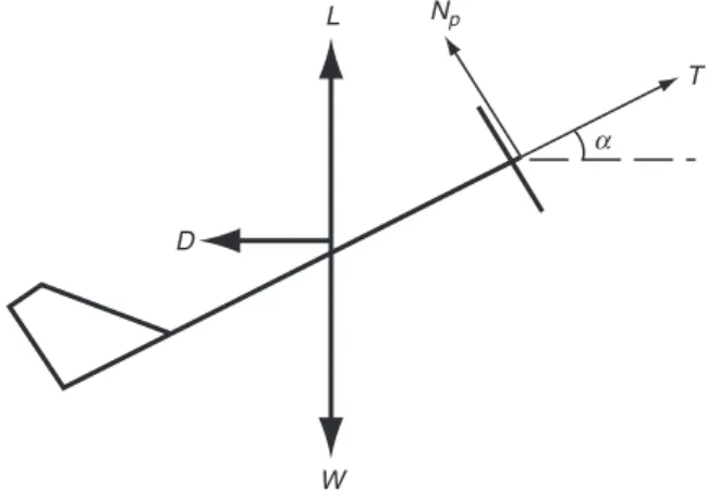
The control variables used in the experiment are elevator angle of deflection, motor rotational speed, and upstream velocity. Angle of attack was held fixed to eliminate hysteresis effects caused by vibration of the model while rotating. Tunnel velocity, elevator deflection, and motor speed were then modified to achieve equilibrium, as described on the Figure 7, that is:

(1) L T Np L W D T Np D M T T y = + + = = − − = = sin cos cos sin α α α α 0 0 Balance measurement sensorex – 2k sensor 4 Conditionning modules ANS E-325

Motor velocity measurement MikroKopter BL-Ctr1 V1.2 XBeePro modem 2.4GHz Data acquisition card

NI PXI-6281

Fiber optic card NI PXI-8336

Pilot and acquisition station Rack NI PXI-1050

ARM7 Control board

F

Fiigguurree 55:: Acquisition System.

0 3 3.05 Thrust (N) 3.1 3.15 3.2 60 10 20 30

Balance angle (deg)

40 50

F

Above, L is lift, W is weight of the vehicle, D is drag, T is thrust, Np is lateral force generated by the propeller and M_yis the moment calculated about the center of gravity. The total lift and drag, L_Tand D_T, represent a summation of all forces in the inertial frame x and z directions, respectively. During testing, velocity was modified until the total lift was equal to the weight. Next, the throttle was changed so the total drag was balanced to zero. Then, the flaps were deflected until the moment was eliminated. However, modifying any of the three control variables resulted in a change in all three measurements. Therefore, multiple iterations of the above process were necessary. Once the equilibrium point was located, the reference or trim velocity was recorded. Additional data were taken by independently modifying the velocity, motor speed, and elevator position from the equilibrium point. Four additional data points were recorded for each variable as described in Table 2. This data will be used to establish near-equilibrium aerodynamic coefficients and control effectiveness.

3. WIND TUNNEL CAMPAIGN RESULTS 3.1. Equilibrium Transition

Velocity, elevator deflection, and motor speed values corresponding to equilibrium were found for angles of attack varying between 15–65 degrees. Below 20 degrees or above 8 m/s, the required motor velocity began to sharply increase. This is accompanied by an increase in required current. Although the aircraft is able to fly higher velocities, it does so at the expense of flight time. The maximum flight speed was not encountered during testing.

At the other end of the spectrum, above 65 degrees, the flow speed of the wind-tunnel descended below 2 m/s, where the quality of the flow is not appropriate for highly sensitive measurements. The equilibrium curves are displayed in Figures 8–10.

These plots represent the trim condition of the aircraft for various angles of attack. Henceforth equilibrium or trim values are represented with the ₀subscript.

Without motors the aircraft would normally stall at 20 degrees angle of attack. However, due to the momentum injected into the flow by the propwash, stall is never encountered. Between 20–40 degrees

α T W D L N_p F

Fiigguurree 77:: Forces applied to the model.

Table 2. Equilibrium investigation

Angle of attack Velocity Rotational speed Aileron deflection

(deg) (m/s) (rad/s) (deg)

Equilibrium point fixed fixed fixed fixed

Upstream velocity sweep Fixed +/−0.3 Fixed Fixed

+/−0.6

Rotational Speed sweep Fixed Fixed +/−0.30 Fixed

+/−0.60

Elevator deflection sweep Fixed Fixed Fixed +/−4

10 9 8 7 6 5 4 Velocity (m/s) 3 2 1 0 0 10 20 30

Angle of attack (deg)

40 50 60 70

F

Fiigguurree 88:: Equilibrium curve Wind-Tunnel Velocity (m/s) for a specified Angle of Attack (deg).

1250

1150

Rotational speed (rad/s)

1050

950

0 10 20 30

Angle of attack (deg)

40 50 60 70

F

Fiigguurree 99:: Equilibrium curve model motor speed (rad/s) for a specified Angle of Attack (deg).

20

10

Elevator deflection (deg)

0

−10

−20

0 10 20 30

Angle of attack (deg)

40 50 60 70

F

angle of attack, corresponding to 7.8–4.6 m/s, the required propeller rotation speed reaches a minimum. This the point at which the least power is required of the motors to maintain equilibrium flight. The cruise speed of the aircraft should be set between 5–8 m/s to increase endurance for long flights. This is also the region where the momentum induced by the propwash is lowest; therefore the danger of stalling the aircraft is likely highest. The controller chosen for the aircraft should avoid sudden decreases in motor speed in this region. An additional conclusion can be drawn from investigation of Figures 8 and 9. Although no data exists for angles of attack lower than 15 degrees, it is seen that the required propeller rotation speed increases dramatically. This indicates a maximum velocity of only 9.5 m/s; rather low for a fixed-wing configuration. The commercial propellers currently used on the MAVion are likely optimized for vertical flight mode with a 3-inch pitch, but present a limitation for cruise flight. Pitch controlled devises may be helpful in future iterations to maintain high propeller performance for all flight modes.

3.2. Near Equilibrium Aerodynamic Model

Once an equilibrium point was found for each angle of attack, data was then taken for near-equilibrium conditions by modifying the velocity, flaps, and motor speed independently. This data was used to explore the sensitivity of the lift, drag, and pitching moment to the various parameter changes. For example, the change in lift due to a change in elevator angle is shown in Figure 11 for several test points. After nondimensionalizing, the slope of this line is the control derivative, C_LTe. Note the T subscript indicates total lift as defined by Equation 1. Figure 12 shows the flap control derivative relationship with angle of attack, along with an appropriate 2nd_{order polynomial fit.}

Lift (N) 2.4 2.6 2.8 3 3.2 3.4 3.6 3.8 4 2.4 2.2 −8 −4 0

Elevator deflection from trim (deg)

4 8

AOA _{= 15°} AOA _{= 25°} AOA _{= 40°} AOA _{= 45°} AOA _{= 65°}

F

Fiigguurree 1111 :: Lift force produced for a given elevator angle (deg) at various angles of attack (deg).

0.1 0.09 0.08 0.07 0.06 0.05 0.04 0.03 0.02 0.01 0 −10 20 30 40 50 60

Angle of attack (deg)

70 o– L T / o – α (N/deg) F

Control derivatives for flap-drag and flap-pitching moment, C_DTeand C_mTe, were also measured. The effect of changing motor rotation speed,ω (rad/s), can also be expressed as control derivatives: C_LTω, C_DTω, and C_mTω. Variations in coefficients due to changes in velocity, C_LTV, C_DTV, C_mTVand are known as stability derivatives. During analysis, it was observed that a velocity squared term was also necessary to model the data: C_LTV2, C_DTV2and C_mTV2. This tendency is likely a result of the complicated interaction between propwash and upstream flow. These twelve derivatives enable calculation of lift, drag, and pitching moment for a given angle of attack, velocity, elevator deflection, and motor speed as demonstrated in Equation 2.

Note that these stability and control derivatives are not defined by a change from zero, but by the perturbations from the trim condition. Resulting force and moment calculations are only valid in regions near equilibrium. Also because at equilibrium the drag and moment are zero, there are no C_DT0 or C_mT0 terms. The derivatives and the zero lift coefficient C_LT0 were determined as polynomial functions of angle of attack. The polynomial coefficients for these functions are listed in Appendix A.

4. CONTROL DURING EQUILIBRIUM TRANSITION

The equilibrium data discovered during the campaign can be immediately applied to the current PID control of the aircraft. Under the assumption that the aircraft is able to maintain near equilibrium conditions during transition, the flight path angle is nearly zero, thus angle of attack is equal to pitch. Knowing motor speed as a function of angle of attack (Figure 9) allows definition of the trim value for throttle as a function of pitch, θ. This relationship can be added directly to the PID altitude loop used to determine throttle setting. Note that if flight path angle is nonzero, this relationship does not hold. For this reason transition flights are not currently performed while modifying the altitude. This assumption may also be affected by the presence of wind. A weak integrator term is used to compensate for steady state errors induced by steady winds. Similarly, the velocity hold calculation benefits from addition of the trim pitch angle as a function of the desired velocity. By further exploring the data obtained from perturbations from equilibrium, however, an entirely different controller may be designed.

Classical control theory uses a linear time invariant (LTI) model to synthesize static or dynamic controllers. It is usually represented by either its state-space form or its transfer function. The relation between both representations is shown by (3).

(3)

However, this representation is only valid in the neighborhood of an equilibrium point. The transition from hover to cruise and vice versa quickly traverses a set of equilibrium points. A representation of the system that enables proof of stability over the whole transition process is desired. Linear Parameter Varying (LPV) models are a suitable choice. Equation (4) shows such a representation where θ (t) is a time-varying vector. When some states of the system are in θ (t) the model is called quasi-LPV.

&x Ax Bu y Cx Du G s D C sI A B = + = +    = + − − , ( ) ( )1 (2) CLT =CLT0( )α +CLTα( )(α α α− 0)+CLTe( )(α e e− 0)+CLTωω α ω ω α α ( )( ) ( )( ) ( )( ) − + − + − 0 0 2 2 0 2 C V V C V V C LTV LTV D DT =CDTα( )(α α α− 0)+CDTe( )(α e e− 0)+CDTω( )(α ω ω− 00 0 2 2 0 2 ) ( )( ) ( )( ) ( + − + − = C V V C V V C C DTV DTV mT mT α α α αα α α)( ) ( )(α ) ω( )(α ω ω ) ( − + − + − + 0 C e e0 C 0 C mTe mT mTV αα)(V−V0)+CmTV2( )(α V −V ) 2 0 2

(4)

It is easy to see the changing dynamics of the MAVion during transition using the pitch angle as a parameter. As a beginning, well-established control methodologies can be used. First stability and performance analysis (µ-analysis [7]) of previously designed controllers guarantees the behavior of the system along the trajectory. Robust synthesis (H_•synthesis) provides tools to optimize a fixed linear dynamic controller such that the closed loop reaches the performance objective. Using a fixed controller to ensure the performance is an ambitious task.

Many aerospace control problems must deal with changing dynamics with operating point. Thanks to some knowledge of the operating point, a fixed controller can be interpolated: this is known as gain–scheduling. For sufficiently slow variation, gain scheduling was shown practically efficient for more than thirty years and later proven theoretically under some hypotheses [8].

Linear Parameter Varying (LPV) controller synthesis methodologies [10] attempt to design a controller explicitly using the information about the current operating point, as described Figure 13. It gives stronger stability results than gain-scheduling.

In order to implement an LPV controller it is necessary to reformulate the model shown in Equation 4 as a Linear Fractional Representation (LFR), pictured shown as the top two blocks in Figure 13.

4.1. Linear Fractional Representation (LFR) Model

The linear fractional representation (LFR) formalism is a theoretical tool that enables one to describe any rational function in some parameters in terms of the feedback interconnection as shown in Figure 14. The variables expressing the rational dependence are grouped in ∆. The reference documentation of the

&x A t x B t u y C t x D t u = + = +    ( ( )) ( ( )) ( ( )) ( ( )) θ θ θ θ ∆ P K ∆ (∆)c F

Fiigguurree 1133:: LPV Control Closed Loop, top half LFR, bottom half controller.

∆

G

w z

u y

F

LFRT 0, a Matlab Toolbox dedicated to the manipulation of such representations, gives an extensive description of this formalism and how to build LFR models.

Any rational function K(δ₁, δ₂, …, δ_N) admits a Linear Fractional Representation:

(5)

with ∆ = diag (δ₁, I_d

1, δ2, Id2, …, δN, IdN)

such that y= K(δ₁,δ₂, … ,δ_N)u. For the present case, K would correspond to the coefficients in Equation 2, while there is only δ₁representing angle of attack.

The transfer between y and u is written F_u(G, ∆)

Transformation is used to separate any time varying or static non-linearities from a nominal linear system. Uncertainties, time-varying parameters or non-linearities complicate any control problem and thus are pulled out in the ∆ block. The LFR consists of a nominal LTI system interconnected with an operator ∆ modeling the uncertainties or other behaviors. The nominal system is described as a LTI system with exogenous inputs and outputs along with the control inputs and measurement outputs. The exogenous outputs are multiplied by an uncertainty block to be then fed back to the inputs. For a more detailed development of how equation 3 relates to Figure 14, the reader may wish to reference Appendix C.

To show how one can transform a polynomial into an LFR, take the lift trim coefficient (6) as an example.

Look for the LFT such that:

(6) Use Hörner factorization and identify the LFR interconnection signals.

This results in the following LFR described by Figure 15:

The LFR set has a convenient property: stability through several algebraic operations such as multiplication, addition and inversion. One can thus build the system dynamic by manipulating LFR of the coefficients. Further details on the link between equations (4) and (5) are provided in Appendix C. (7) C a b c d e e d c b a L z 0 4 3 2 1 ( ) ( ( ( ) θ θ θ θ θ θ θ θ θ = + + + + = + + + _{+ {{} 124 34 1 244 443 144424443 z z z 2 3 4 )) y=CL0( )θ u=Fu( , ) ,G ∆u with ∆= ⋅θ I z G w G u y G w G u w z G G G G G = + = +    = = 11 12 21 22 11 12 21 2 , ∆ 2 2       θ 0 0 0 0 θ 0 0 0 0 θ 0 0 0 0 θ 0 0 0 0 1 0 0 0 0 1 0 0 0 0 0 1 1 a z w u _{= 1} y = C_L0 b c d e 0 0 0 F

4.2. Linearization

It is desirable to form a linear model of the form shown in Equation 3. Taking the state and control vectors to be as follows:

(8)

Here, θ is the pitch angle. Again, assuming near equilibrium conditions and very small wind perturbation, this is equal to the angle of attack as indicated previously. q is the pitching rate in radians per second, V is the aircraft inertial frame horizontal velocity and V_zis the vertical velocity also in the inertial frame. The control variables are e, elevator in radians and ω, motor rotational velocity in radians per second. The rate vector can be defined in terms of the aerodynamic coefficients:

Equation 9 represents a non-linear model of the behavior of the aircraft, however, the aerodynamic coefficients are only identified near equilibrium suggesting a linearized model is needed. The rate vector for x can be linearized as:

The derivatives are then separable into the A and B matrices found in Equation 11–12:

(12) B q e q V e V V e V z z = ∂ ∂ ∂ ∂ ∂ ∂ ∂ ∂ ∂ ∂ ∂ ∂        0 0 & & & & & & ω ω ω                (11) A q q V V V V V V V z z = ∂ ∂ ∂ ∂ ∂ ∂ ∂ ∂ ∂ ∂ ∂ ∂ 0 1 0 0 0 0 0 0 0 & & & & & & θ θ θ 00                       (10) &

& & & &

x q q e e q q V V = ∂ ∂ ∂ + ∂∂ ∂ + ∂∂ ∂ + ∂∂ ∂ ∂ θ( θ) ( ) ω( ω) ( ) && & & &

& V V e e V V V V V_z ∂ ∂ + ∂∂ ∂ + ∂∂ ∂ + ∂∂ ∂ ∂ θ( θ) ( ) ω( ω) ( ) ∂∂ ∂ + ∂ ∂ ∂ + ∂ ∂ ∂ + ∂ ∂ ∂   θ θ ω ω

( ) V& ( ) & ( ) & ( )

e e V V V V z z z q                   (9) &x J S L V C m S V yy ref ref mT q ref =         1 1 2 1 1 2 2 2 ρ ρ CC m S V C DT ref LT                    1 1 2 2 ρ            x q V V u e z T T = = [ ] [ ] θ ω

Combining this linearization to the relationships in Equation 10, one can define expressions for the above derivatives. These are presented in Appendix B. The first derivative is provided as an example:

(13)

The twelve derivatives contained in A and B vary as functions of pitch. As each coefficient and equilibrium parameter is a fourth order polynomial, the derivative is a nineteenth order polynomial and the ∆ block of the associated LFR will be of equal size. The dimension of the ∆ block is critical to the success of the numerical procedures used for controller synthesis. Additionally, this model, though nonlinear in the parameter, is a family of linearization and in such remains valid only if the states and inputs stay near the equilibrium trajectory.

5. CONCLUSION AND FUTURE WORKS

A wind tunnel campaign was performed to reveal the trim state of a fixed wing VTOL MAV during the transition between horizontal and vertical flight modes. Further exploration of perturbations around the trim state yielded a linearized model whose stability and control derivatives are functions of angle of attack. The model has been expressed in Linear Fractional Representation as a first step for use in adaptive control methods such as LPV.

Future aerodynamic testing will investigate the specific nature of the flow. Propwash impingement on the wing, swirl effects, and stall are areas requiring more detailed studies. Numerical simulations are also in progress to validate the trim model and evaluate the blockage effect in the wind-tunnel test section. A structured C-grid with an actuator disk is used to model the aircraft and the propellers as shown Figure 16. The end goal of the aerodynamic testing and controls development presented here is to produce aircraft uniquely capable of vertical and horizontal flight modes. Several prototypes have already been constructed and outfitted with autopilots developed at ISAE. There are two varieties of the aircraft in development. The first is equipped with GPS for outdoor navigation, and has demonstrated fully autonomous transitions between vertical and horizontal flight. It is able to drop a small payload and auto take-off and land.

The second version, destined for mostly indoor flight, has carbon fibre wheels attached which are used to roll along the ground, walls, and ceilings guided by an attached camera using First Person

∂ ∂ = − ∂ ∂ − ∂ ∂ − &q J S L V C e C C yy ref ref me me θ ρ θ ω θ 1 2 0 2 0 0 m mV mV V C V V ∂ ∂ − ∂ ∂             0 2 0 0 2 θ θ F

Vision (FPV). Both versions featuring quaternion-based PID controllers for stability have been successfully flown at IMAV 2011. Future work will utilize the model that has been developed here to implement modern adaptive controllers to improve the performance of the aircraft as it transtitions between vertical and horizontal flight modes.

ACKNOWLEDGEMENTS

The present work has been partially supported by the Pôle de recherche et d’enseignement supérieur (PRES) of the University of Toulouse, the European Office for Aerospace Research and Development (EOARD), the Direction Générale de l’Armement (DGA-MRIS) and the US Air Force. The authors would like to express their gratitude for the contribution of Sylvain Masseboeuf in conducting the wind tunnel experiments and to thank the other members of the ISAE for their involvement to this work: Rémi Chanton, Xavier Foulquier, Serge Gérard, Marc Grellet, Guy Mirabel, Patrick Morel and Serge Moretti. For their helpful discussions and contributions to the present study, the authors would also like to thank the students: Roméo Brogna, Hugo Martin, Mathieu Melgrani and Amelie Peyret.

REFERENCES

[1] C. Thypiopas, B. Bataillé, J.M. Moschetta. A Fixed Wing Micro Air Vehicle for Transition Flight: Aerodynamic and Propulsion Study. IMAV Conference, Pensacola, Florida USA, July 2009.

[2] R. Carr, J.M. Moschetta, C. Thipyopas, G. Mehta. IMAV Conference 2010, Braunschweig, Germany, July 2010.

[3] R.H. Stone and G. Clarke. Optimization of Transition Manoeuvres for a Tail-Sitter Unmanned Air Vehicle (UAV). Australian International Aerospace Congress, Canberra, Australia, 2001. [4] S. Masseboeuf. Manuel d’Utilisation de la Soufflerie Sabre. Internal publication for ISAE,

Toulouse, France, November 2010.

[5] A. Krynytzky. Classical Corrections for Closed Test Sections. In B.F.R. Ewald, editors, Advisory Group for Aerospace Research & Development, Darmstadt University of Technology, Federal Republic of Germany, volume 336, pages 2–13 – 2–35. Canada Communication Group Inc., 1998.

[6] J. Magni, User Manual of the Linear Fractional Representation Toolbox Version 2.0. Onera DCSD.

[7] John C. Doyle; Structured uncertainty in control system design, Decision and Control, 1985 24th IEEE Conference on, vol. 24, no., pp. 260–265, Dec. 1985.

[8] J. S. Shamma, Analysis and design of gain scheduled control systems, Phd Thesis 1988. [9] C. W. Scherer, LPV control and full block multipliers, Automatica, vol. 37, no. 3, pp. 361–375,

2001.

[10] P. Apkarian and P. Gahinet, A convex characterization of gain-scheduled H infinity controllers,

F

Fiigguurree 1177 :: Two MAVion prototypes. At left is the outdoor GPS equipped version. At right is the wheeled version for indoor vision based flight.

IEEE Transactions on Automatic Control, vol. 40, pp. 853–864, may 1995.

APPENDIX A. POLYNAMIAL COEFFICIENTS FOR FUNCTIONS OF PITCH ANGLE

The polynomials are represented as follows:

a b c d e

V₀ 5,97E + 01 −1,63E + 02 1,63E + 02 −7,82E + 01 2,13E + 01

e₀ −1,07E + 01 2,96E + 01 −2,71E + 01 9,43 1,03

ω0 4,67E + 06 −9,96E + 03 1,10E + 04 −5,38E + 03 1,97E + 03

C_LT0 −2,07E + 01 9,96E + 01 −1,07E + 02 4,54E + 01 −5,58 C_LTe 3,12E + 01 −7,03E + 01 5,54E + 01 −2,04E + 01 9,55E – 01 C_LTω 5,20E – 03 4,16E – 02 −5,89E – 02 2,91E – 02 −4,00E – 03 C_LTV −8,57E + 02 1,82E + 03 −1,40E + 03 4,51E + 02 −5,14E + 01 C_LTV2 2,09E + 02 −4,58E + 02 3,60E + 02 −1,19E + 02 1,38E + 01 C_DTe 2,45E + 01 −8,85E + 01 8,88E + 01 −3,69E + 01 4,64 C_Dω 3,57E – 02 −1,03E – 01 9,51E – 02 −3,72E – 02 4,30E – 03 C_DTV −2,60E + 02 7,25E + 02 −6,64E + 02 2,47E + 02 −3,08E + 01 C_DTV2 3,40E + 01 −1,03E + 02 9,88E + 01 −3,77E + 01 4,84 C_mTe −1,70E + 01 3,32E + 01 −2,51E + 01 8,15 −3,83E – 01 C_mTω −9,00E – 05 −1,64E – 02 2,25E – 02 −1,05E – 02 1,40E – 03 C_mTV −1,60E + 02 4,61E + 02 −4,33E + 02 1,63E + 02 −2,06E + 01 C_mTV2 1,53E + 01 −5,02E + 01 5,02E + 01 −1,95E + 01 2,53

with θ in radians.

V0 a b c d e

4 3 2

APPENDIX B. STABILITY AND CONTROL DERIVATIVES

The polynomials are represented as follows:

(B.3) ∂ ∂ = ∂ ∂ − ∂ ∂ − ∂ &V m S V C C e C z ref LT LTe LTe θ ρ θ θ ω 1 2 0 2 0 0 ' 00 0 2 0 0 2 ∂ − ∂ ∂ − ∂ ∂             ∂ θ θ θ CLTV V CLTV V V ' &VV V m S V C V C V e m z ref LTV LTV z ∂ =

[

+

]

∂ ∂ = 1 2 2 1 2 0 2 0 2 ρ ρ & S S V C V m S V ref LTe z ref 0 2 0 2 1 2    ∂ ∂ =   ( )θ ω ρ & CLTω( )θ (B.2) ∂ ∂ = ∂ ∂ − ∂ ∂ − ∂ &V m S V C C e C ref DT DTe DTe θ ρ θ θ ω 1 2 0 2 0 0 0 ' ∂∂ − ∂ ∂ − ∂ ∂             ∂ θ θ θ C V C V V V DTV DTV 0 2 0 0 2 ' & ∂∂ =

[

+

]

∂ ∂ = V m S V C V C V e m S ref DTV DTV re 1 2 2 1 2 0 2 0 2 ρ ρ & ff DTe ref D V C V m S V C 0 2 0 2 1 2    ∂ ∂ =   ( )θ ω ρ & T Tω( )θ (B.1) ∂ ∂ = − ∂ ∂ − ∂ ∂ − &q J S L V C e C yy ref ref me me θ ρ θ ω θ 1 2 0 2 0 0 ' C C V C V V q V mV mV ∂ ∂ − ∂ ∂             ∂ ∂ = 0 2 0 0 2 1 2 θ θ ' & JJ S L V C V C q e J yy ref ref mTV mTV yy ρ ρ 0 2 0 2 2 1 2 +

[

]

∂ ∂ = & S S L V C q J S L

ref ref mTe

yy ref r 0 2 1 2     ∂ ∂ = ( )θ ω ρ & eefV0 CmT 2     ω( )θ

APPENDIX C. STABILITY AND CONTROL DERIVATIVES

Any rational function K(δ₁, δ₂, …, δ_N) admits a Linear Fractional Representation:

x· x y A B C D u 1 s F

Fiigguurree CC22:: Dynamic System.

such that y= K(δ₁, δ₂, …, δ_N)u

The transfer between y and u is written F_u(G, ∆).

Equation (C.1) represents the most general case of a LFR. The ∆ block contains only static parameters but using the integrator operator, 1/s, dynamical system can be represented. The state space representation of a system can then be seen as the LFR of G(s) with ∆ = 1/sI_n, and n the number of states of the system.

(C.2)

The state-space matrices may depend on a parameter vector θ as described by Equation (C.3).

(C.3)

Provided that this dependence is rational, an LFR can be derived. First, the following notations are introduced: (C.4) % & % y x y u x u K A B C D T T =

[ ]

=

[ ]

=     , ( ) ( ) ( ) ( ) θ θ θ θ &x A t x B t u y C t x D t u = + = +    ( ( )) ( ( )) ( ( )) ( ( )) θ θ θ θ &x Ax Bu y Cx u G s D C sI A B = + = +    = + − − ( ) ( )1 (C.1) z G w G u y G w G u w z G G G G G = + = +    = = 11 12 21 22 11 12 21 , ∆ , 2 22 0 0 0 0 0 0 1 1 2 2    _ =     ∆ δ δ δ I I I d d N dN L K M M O M L           ∆ w G z u y F

K admits a LFR representation such that G is usually decomposed as follows:

(C.5)

After a suitable vector reordering, this formulation leads to the traditional notation for a LFR state-space system found in the literature:

(C.6)

The original state-space matrices can be expressed using the new variables by closing the loop with the ∆ block. The state space matrices of equation (4) then become:

(C.7)

In turn, if the loop is closed around the integrator operator, a transfer function can be derived:

(C.8) ∆ M (s ) w u z y G s C sI A B D G s C sI A B 11 1 1 1 11 12 1 1 ( ) ( ) ( ) ( ) = − + = − − − % % _{22 12} 21 2 1 1 21 22 2 + = − + = − − D G s C sI A B D G s C sI ( ) ( ) ( ) ( % %%A B D)−1 + 2 22 A( ) ( ) ( ) ( ) θ θ = + − = + − − − %A B I D C B B B I D 1 11 1 1 2 1 11 1 ∆ ∆ ∆ ∆∆ ∆ ∆ D C C D I D C D D D I 12 2 21 11 1 1 22 21 ( ) ( ) ( ) ( θ θ = + − = + − −−_∆ −_∆ D11 D 1 12 ) & % x z y A B B C D D C D D           =       1 2 1 11 12 2 21 22              x w u ∆ M x w x· z u y 1 s z x y D C D B A B D C D & %           =       11 1 12 1 2 21 2 22              w x u % % y=F Gu( , )∆ u⋅ % & u A B C D x u x y  →  →      →  →    ( ) ( ) ( ) ( ) θ θ θ θ _%y