Science Arts & Métiers (SAM)
is an open access repository that collects the work of Arts et Métiers Institute of Technology researchers and makes it freely available over the web where possible.
This is an author-deposited version published in: https://sam.ensam.eu
Handle ID: .http://hdl.handle.net/10985/10377
To cite this version :
Ouadie HMAD, Nazih MECHBAL, Marc REBILLAT - Peaks Over Threshold Method for Structural Health Monitoring Detector Design - In: 10th International Workshop on Structural Health
Monitoring, Etats-Unis, 2015-09 - International Workshop on Structural Health Monitoring - 2015
Any correspondence concerning this service should be sent to the repository Administrator : [email protected]
ABSTRACT1
Structural Health Monitoring (SHM) system offers new approaches to interrogate the integrity of structures. The most critical step of such systems is the damage detection step since it is the first and because performances of the following steps (damage localization, severity estimation…) depend on it. Care has thus to be taken when designing the detector. The objective of this communication is to discuss issues related to the design of a detector for the structural health monitoring of composite structures. The structure under monitoring is a substructure of an aircraft nacelle. In the absence of damage, the detector principle is to statistically characterize the healthy behavior of the structure. This characterization is based on the availability of a decision statistics synthesized from a damage index. Airline business models rely on Probability of False Alarms (𝑃 𝑎) as main performance criterion. In general, the requirement on 𝑃 𝑎 is 10E-9 which is very small. To determine the decision threshold, the approach we consider, consists to model the tail of the decision statistics using the Peaks Over Threshold method extracted from the extreme value theory (EVT). This method has been applied for different configuration of learning sample and probability of false alarm. This approach of tail distribution estimation is interesting since it is not necessary to know the distribution of the decision statistic to develop a detector. However, its main drawback is that it is necessary to have very large databases to accurately estimate decision thresholds to then decide the presence or absence of damage.
INTRODUCTION
One of the major concerns of airlines is the availability of their equipment. The unavailability of a plane with passenger on board is among the worst situations. Many solutions are implemented to avoid this, like Structural Health Monitoring (SHM) systems [1]. The most critical step of such systems is the damage detection step since it is the first step of the process and because performances of the following steps (damage localization, severity estimation…) depend on it. The detector has thus to be well designed in order to ensure optimal system performances.
In order to design a SHM detector, two issues have to be solved. The first one is the choice of the Damage Index (DI) to consider and the second one is the way to use it for detection purposes. A detector design thus does not reside solely in the DI choice and implementation but also includes the processing steps needed to compute a decision statistic using the DI estimations. The final step then consists in deciding the presence or absence of a damage.
The performance of SHM detector depends on a decision threshold to be applied to the decision statistic [2]. The decision threshold has to be determined according to a tradeoff between errors of type I and errors of type II. The type I error represents the probability to detect a damage when the structure is healthy - P(Detection|Healthy) (probability of false alarm - pfa). The type II error represents the probability to detect a damage when the structure is faulty or damaged - P(Detection|Faulty) (probability of detection - PoD).
Ouadie HMAD, Nazih MECHBAL and Marc REBILLAT, PIMM UMR CNRS, Arts et Métiers ParisTech, 151 boulevard de l’Hôpital, 75013Paris, France
Airline business models rely on Probability of False Alarms (𝑝 𝑎) [3], which is the type I error, as main performance criterion. In general, the requirement on 𝑃 𝑎 is 10E-9 which is very small. To determine the decision threshold, a first approach consists in estimating the probability density of the overall decision statistics and to work with this estimate. In this case, parametric and nonparametric density estimation methods can be used [4]. A second approach, that we consider, consists to only estimate the tail of the decision statistics. In this case, the extreme value theory (EVT) is used [5].
This paper is structured as follows: first, the structure under monitoring is presented in order to understand the experimental setup. Then the considered damage index is defined and the decision statistic computation is explained. After that, the Peaks Over Threshold method is introduced to estimate the decision statistic tail distribution. Finally, results are presented for several configurations of learning samples and probability of false alarm values before concluding.
THE MONITORED STRUCTURE
The structure under monitoring is an aircraft nacelle (Figure 1(a)). Aircraft nacelles represent a critical part of an aircraft as they perform multiple functions. They contribute to the braking of the plane on landing and reduce noise emissions in drastically severe conditions including extreme temperatures [-50°C +150°C], pressure and dimension constraints, whilst remaining as light as possible.
Before working on the overall nacelle structure, we first work on representative specimens. The considered specimen is a laminate carbon epoxy plate, part of the structure, of dimension 400mm×300mm (Figure 1(b)). It represents the laboratory step of the implementation of a health monitoring process for the actual aircraft nacelle [6]. A network of actuators and sensors bonded on the surface is used to collect data. The monitoring of the structure is based on the comparison of the data recorded for a healthy state (baseline) and an unknown state. The data of the host structure are collected thanks to piezoelectric transducer (PZT) and a real-time diagnosis result is obtained. The PZT elements used were numbered 1 through 5 and mounted at specific positions on the composite plate’s surface [7]. The PZT elements have a diameter of 20mm and a thickness of 0.1mm. Figure 1(c) shows the location of the 5 PZT discs and the coordinate values in x and y directions.
(a) (b) (c)
Figure 1. (a) The aircraft nacelle; (b) A flat view of Laminate Carbon epoxy with PZT elements; (c) PZT coordinates on the composite plate’s surface
DAMAGE INDEX AND DECISION STATISTIC
The damage index represents a crucial step for the design of the detector. It therefore must correctly reflect the effect of damage on the structure. The damage index chosen for this communication is obtained as follows:
For one actuator - sensor path:
1. A signal is sent from the PZT actuator (Act PZT)
2. The received signal on the PZT sensor (Sens PZT) is then recorded 3. This signal undergoes a denoising phase (wavelet denoising and
time-frequency filtering)
4. Its envelope is computed thanks to a Hilbert transform.
These steps have been performed for each actuator-sensor path 500 times in a healthy situation. In the absence of damage, the objective is to characterize the healthy
behavior of the structure to define a detector without having to damage several structures.
Subsequently, each of the signals for which the envelope was computed is considered as reference (sigref(i)) and is compared to the other signals that are
considered as test signals (sigtest(j)) as follows:
𝐼 ; =
‖ − ‖
‖ ‖ ℎ ≠ (1)
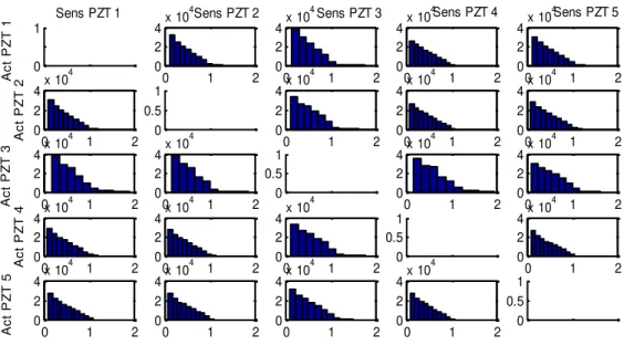
By rotating the reference signal and the test signals, a database of 124750 DI is obtained and allows characterizing the healthy behavior of the structure. Figure 2 shows the histograms of the DI for each actuator-sensor path. These histograms represent the distributions for each actuator-sensor path when the structure is healthy. The diagonal is empty since the sent signal is the same as the received one because the actuator is the sensor.
Figure 2. Histograms of the DI for each actuator-sensor path.
As an example, Figure 3 represents the histogram of the DI for the actuator 1 – sensor 5 path. This figure represents the distribution of the decision statistic for this path.
Figure 3. Decision statistic histogram for actuator 1 – sensor 5 path.
ESTIMATION OF THE DECISION STATISTIC AND DECISION THRESHOLD
The performance of a detector depends on a decision threshold to be applied to a decision statistics. This threshold has to be determined according to a requested probability which defines the first order error (probability of false alarm - 𝑝 𝑎). To determine the decision threshold, a first approach consists in estimating the probability
0 1 Sens PZT 1 A c t P Z T 1 0 1 2 0 2 4x 10 4Sens PZT 2 0 1 2 0 2 4x 10 4Sens PZT 3 0 1 2 0 2 4x 10 4Sens PZT 4 0 1 2 0 2 4x 10 4Sens PZT 5 0 1 2 0 2 4x 10 4 A c t P Z T 2 0 0.5 1 0 1 2 0 2 4x 10 4 0 1 2 0 2 4x 10 4 0 1 2 0 2 4x 10 4 0 1 2 0 2 4x 10 4 A c t P Z T 3 0 1 2 0 2 4x 10 4 0 0.5 1 0 1 2 0 2 4x 10 4 0 1 2 0 2 4x 10 4 0 1 2 0 2 4x 10 4 A c t P Z T 4 0 1 2 0 2 4x 10 4 0 1 2 0 2 4x 10 4 0 0.5 1 0 1 2 0 2 4x 10 4 0 1 2 0 2 4x 10 4 A c t P Z T 5 0 1 2 0 2 4x 10 4 0 1 2 0 2 4x 10 4 0 1 2 0 2 4x 10 4 0 0.5 1 0 0.2 0.4 0.6 0.8 1 1.2 1.4 0 0.5 1 1.5 2 2.5 3 3.5x 10 4 DI values Actuator 1 - Sensor 5
density of the overall decision statistics and to work with this estimate [4]. In this case, parametric and nonparametric density estimation methods can be used. A second approach consists to only estimate the tail of the decision statistics. In this case, the extreme value theory is used [5].
Extreme value theory (EVT) is often applied when it is necessary to estimate rare events despite the fact that the distribution of the studied sample is unknown. The interest is credited on the asymptotic behavior of the extreme values of a sample. Thus by identifying the distribution family to which extreme values will converge [8] (domain of attraction of the maximum – DAM: Fréchet, Weibull or Gumbel) (Figure 4), it is possible to use its distribution function.
Figure 4. Domain of Attraction of the Maximum – DAM : Fréchet, Weibull or Gumbel To characterize the DAM of the extremes, two theorems are essential:
Fisher-Tippet theorem [5]
Balkema-Haan-Pickands theorem [9].
These two theorems have resulted in two distribution tails estimation methods: the method of the maxima per blocks (Block Maxima - BM) that models
the distribution of standardized maxima by the generalized extreme value distribution (GEV), an adaptation of this method have been used in [10] and [11]
the method of excess (Peaks Over Threshold - POT) [12] that models the distribution of the excess beyond a learning threshold by the generalized Pareto distribution (GPD).
Here we applied the POT method to estimate the distribution of the decision statistic for each actuator-sensor path and to then determine decision thresholds for each actuator-sensor path.
PEAKS OVER THRESHOLD METHOD
The Peaks Over Threshold (POT) method [12], also called method of excess, focuses on the distribution of the excess above a high learning threshold. This modeling of the distribution tail is based on the theorem of Balkema-Haan-Pickands [9] [13] which is the equivalent of the central limit theorem for the extreme value theory.
This theorem states that if a decision statistic distribution belongs to one of the three domain of attraction (Fréchet, Weibull or Gumbel), then there exists a distribution function of the excess above a high learning threshold , denoted , which can be approximated by a generalized Pareto distribution (GPD) [5].
The generalized Pareto distribution of parameters ξ and β is defined by the following distribution function:
(2)
with 𝛽 > . For 𝜉 ≥ , the distribution support is [ ; + ∞[. When 𝜉 < , the distribution support is [ ; − 𝛽/𝜉].
The generalized Pareto distribution comprises three types of distributions limits according to the values of the shape parameter 𝜉:
P ro b a b ili ty d e n s it y > 0, Frechet DAM < 0, Weibull DAM = 0, Gumbel DAM 𝜉,𝛽 = 1 − 1 +𝜉 𝛽 −1 𝜉 𝜉 ≠ 0 1− 𝑝 − 𝛽 𝜉 = 0
if 𝜉 > , standard Pareto distribution (Frechet DAM), if 𝜉 < , Pareto distribution of type II (Weibull DAM), if 𝜉 = , exponential distribution (Gumbel DAM).
Before estimating the model, we must build a suitable excess sample. It is therefore necessary to find a learning threshold to select sufficient high extreme data and above which enough data are preserved for accurate estimates. If the learning threshold is too low, the estimates are biased and if the learning threshold is too high, the variance of the estimators is very important.
The method of excess (POT) consists in setting a learning threshold large enough to be applied to each learning sample (𝑁: the decision statistic) in order to define a sample of excess (𝑁 ) for each learning sample. The generalized Pareto distribution parameters are then estimated by maximum likelihood [14] from the sample of excess.
What particularly interests us in this study concerns the estimation of extreme quantiles, which represent decision thresholds, from the parameter estimates of the GPD. To do this, it is possible to use a semi-parametric estimator of quantiles from the POT method which has been obtained by inverting the distribution function of the GPD [15]. This enables to determine the value of a quantile (wich is the decision threshold S) corresponding to a probability of false alarm (𝑝 𝑎). This estimator is expressed as follows: 𝑆 ̂𝑝 𝑎= +𝛽̂ 𝜉̂ ( 𝑁 𝑁 − 𝑝 𝑎 ) −𝜉̂ − (3)
with 𝑁 the number of excess beyond the learning threshold , N the learning sample size, 𝛽̂ and 𝜉̂ estimated values (by maximum likelihood) of the generalized Pareto distribution parameters.
This estimator has been used to determine the decision thresholds for 𝑝 𝑎 = { − ; − ; − }. The experiment has been conducted on the basis of the previously obtained DI. Different sizes of learning samples were tested: 𝑁 =
{ ; ; ; } which corresponds respectively to
approximately 0.25 * 124750, 0.5 * 124750, 0.75 * 124750 and 1 * 124750. As the learning threshold is unknown a priori, different values for which the size of the samples of excess ranging from 1% to 10% of the total size of the learning samples 𝑁 were tested to determine the parameters of the generalized Pareto distribution. Subsequently, decision thresholds have been estimated.
In order to compare the POT thresholds (estimated decision thresholds), we considered a nonparametric Parzen window estimator [16] as reference and determine decision thresholds that have to be considered as reference for the same configuration described before. Before showing results, the Parzen estimator is described below. PARZEN WINDOW ESTIMATOR
The Parzen window [17] adjustment is a nonparametric mean to estimate the probability density function of a random variable 𝑌 (here, the decision statistic). It is commonly named kernel density estimator [13] because kernel functions are used to estimate the probability density function. The analytical expression of the nonparametric probability density function is [18]:
(11)
Where 𝐾 and are the kernel function and the window width, respectively. The idea behind the Parzen window is to estimate the density probability function on each decision statistic value thanks to a kernel function 𝐾 . which is most of the time a probability density function. The closer the observation is to training samples 𝑖 the larger is the contribution to ̂ℎ the kernel function centered on 𝑖. Conversely, training observations 𝑖 that are far from have a negligible contribution to ̂ℎ. This estimator of the probability density function is formed by averaging of the kernel function values (Figure 5).
N i i h h y y K h N y f 1 * 1 ) ( ˆFigure 5. Probability density function of a random variable and some Gaussian kernels. This estimator is governed by a smoothing parameter ℎ which is named window width. The estimation of a probability density function, which depends on the smoothing parameter ℎ, presents good statistical properties. Under some non-binding restrictions on ℎ, the Parzen window estimator is consistent. It exist several kernel functions (Gaussian, box, triangle…) but the Parzen window performance depend principally on the choice of the window width ℎ [19]. A tradeoff between the bias and the variance of the estimator must be determined to choose ℎ. It exist several methods to choose ℎ. The window width can be chosen thanks to cross validation or by maximizing the likelihood of the kernel function for example. In this study, a Gaussian kernel has been used. Silverman [18] has determined the optimal smoothing parameter value called “rule of thumb” when the distribution is Gaussian. This window width depends on an estimation of the variance and the learning data set size.
RESULTS
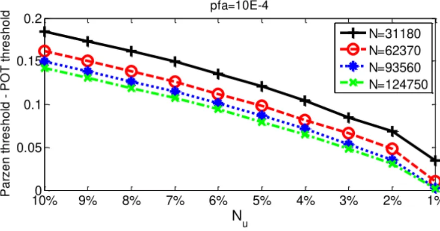
In order to compare the results of estimates of distribution tails the non-parametric Parzen window estimation has been applied to the same learning samples. Then the difference between the Parzen thresholds (reference) and the POT thresholds (test) has been computed. This difference is then plotted for several 𝑝 𝑎 and learning samples size (𝑁) values against the excess sample sizes (𝑁 ) as a percent of 𝑁.
The following figures represent the difference of Parzen thresholds and POT thresholds for several different configurations for actuator 1 – sensor 5 path. The x-axes represent the excess sample sizes (𝑁 ), used for the estimation of the generalized Pareto distribution parameters. The excess sample size is rounded to the integer of the actual theoretical size.
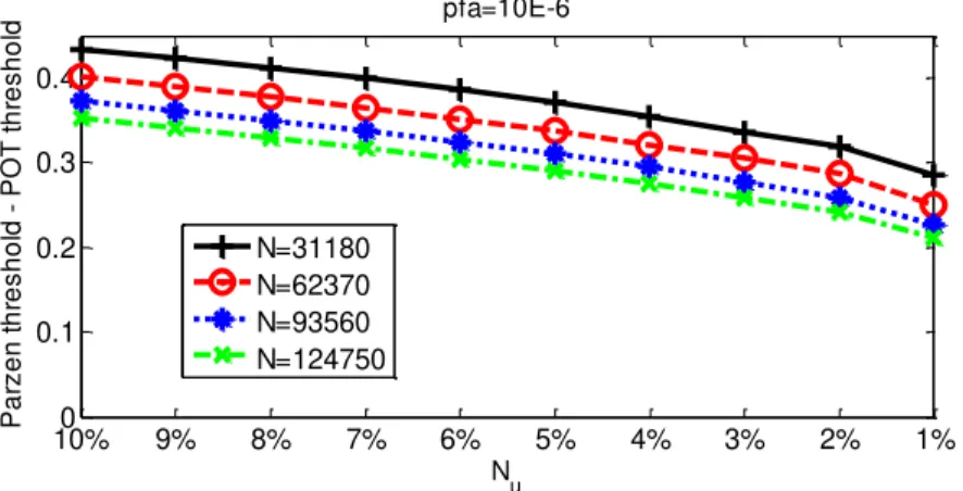
Figure 6 shows that whichever the learning sample size N, when 𝑁 decreases, the difference between Parzen thresholds and POT thresholds become close to zero. It can be explained by the fact that when the learning threshold increases, the DAM is well represented by the sample of the excess as explained in the POT description. This observation means that bigger the learning threshold better the estimation of the decision thresholds. However, when 𝑝 𝑎 decreases, Figure 7 and Figure 8 show that this difference increases and depart from zero. It means that despite of the large size of the learning samples, when we look for a very small value of 𝑝 𝑎, we need a much bigger learning sample than those available. Using the EVT needs thus a very large amount of data when looking for very low first order error.
Figure 6. Parzen threshold – POT threshold estimated on excess sample size Nu of 1% to 10% of 4 different learning sample sizes N for 𝑝 𝑎 = E − .
10%0 9% 8% 7% 6% 5% 4% 3% 2% 1% 0.05 0.1 0.15 0.2 Nu P a rz e n t h re s h o ld P O T t h re s h o ld pfa=10E-4 N=31180 N=62370 N=93560 N=124750
Figure 7. Parzen threshold – POT threshold estimated on excess sample size Nu of 1% to 10% of 4 different learning sample sizes N for 𝑝 𝑎 = − .
Figure 8. Parzen threshold – POT threshold estimated on excess sample size Nu of 1% to 10% of 4 different learning sample sizes N for 𝑝 𝑎 = − .
CONCLUSION
The objective of this communication is the design of a detector for the health monitoring of composite structures. The structure under monitoring is a substructure of an aircraft nacelle. In the absence of damage, the detector principle is to statistically characterize the healthy behavior of the structure. This characterization is based on the availability of a decision statistics synthesized from a damage index.
Once the decision statistic is available, the POT method has been used to determine decision thresholds in only considering the tail of the decision statistic. This has been done for different configuration of learning sample and probability of false alarm for each actuator – sensor path. In addition, a Parzen window has been used and acts as a reference to compare the estimated POT thresholds to those obtained by Parzen.
The results show that for a total sample size of 124750, only the thresholds estimated for 𝑝 𝑎 = − are correctly estimated when the size of the excess sample represents 1% of the total size of the learning sample. More the 𝑝 𝑎 decreases more the gap widens. This implies that it is necessary to increase the learning sample size when 𝑝 𝑎 decreases.
This approach of tail distribution estimation is interesting since it is not necessary to know the distribution of the decision statistic to develop a detector. This represents a real issue in the industry where the distribution of decision statistics is unknown due to the complexity of the studied systems and structures. On the other hand, the main drawback of this approach is that it is necessary to have very large databases to accurately estimate decision thresholds to then decide the presence or absence of damage.
REFERENCES
1. T. Massot, M. Guskov, C. Fendzi, M. Rebillat and N. Mechbal, "Structural Health Monitoring Process for Aircraft Nacelle," in ACMA, Marrackech, 2014.
2. C. Fendzi, J. Morel, M. Rébillat, M. Guskov, N. Mechbal and G. Coffignal, "Optimal Sensors
10%0 9% 8% 7% 6% 5% 4% 3% 2% 1% 0.1 0.2 0.3 0.4 Nu P a rz e n t h re s h o ld P O T t h re s h o ld pfa=10E-6 N=31180 N=62370 N=93560 N=124750 10%0 9% 8% 7% 6% 5% 4% 3% 2% 1% 0.2 0.4 0.6 0.8 Nu P a rz e n t h re s h o ld P O T t h re s h o ld pfa=10E-9 N=31180 N=62370 N=93560 N=124750
Placement to Enhance Damage Detection in Composite Plates," European Workshop on Structural health Monitoring, Nantes, 2014.
3. C. Hemez, M. Czarneckif, J. Shunk, D. Stinemates, D. Sohn, H. Farrar and B. Nalder, "A review of structural health monitoring literature : 1996-2001," Los Alamos National Laboratory Report, 2003. 4. O. Hmad, E. Grall-Maës, P. Beauseroy, J.-R. Masse and A. Mathevet, "A comparison of
distribution estimators used to determine a degradation decision threshold for very low first order error," in ESREL conference, Troyes, 2011.
5 O. Hmad, E. Grall-Maës, P. Beauseroy, J.-R. Masse and A. Mathevet, "Maturation of Detection Functions by Performances Benchmark. Application to a PHM Algorithm," in Prognostics and
System Health Management Conference, Milan, Italy, 2013.
6. J. Pickands, «Statistical inference using extreme order statistics,» Annals of statistics, vol. 3, pp. 119-131, 1975.
7. A. McNeil and T. Saladin, The peaks over thresholds method for estimating high quantiles of loss
distributions, 1997.
8. M. Lejeune, Statistique : La théorie et ses applications, Paris: Springer, 2010.
9. J. Hosking et J. et Wallis, «Parameter and quantile estimation for the generalized Pareto distribution,» Technometrics, vol. 29, pp. 339-349, 1987.
10. J. Hosking, «Maximum-likelihood estimation of the parameters of the generalized extreme-value distribution,» Applied Statistics, vol. 34, pp. 301-310, 1985.
11. E. Gumbel, Statistics of Extremes, New York: Columbia University Press, 1958. 12. R. Duda, P. Hart et D. Stork, Pattern classification, New York: Wiley, 2001.
13. L. De Haan et H. Rootzen, «On the estimation of high quantiles,» J. Statist. Plann. Inference, vol. 35, pp. 1-13, 1993.
14. S. Coles, An Introduction to Statistical Modeling of Extremes Values, London: Springer, 2001. 15. W. S. H. Park, «Parameter estimation of the generalized extreme value distribution for structural
health monitoring,» Probabilistic Engineering Mechanics, vol. 21, pp. 366-376, 2006.
16. H. Sohn, D. Allen, K. Worden et C. Farrar, «Structural Damage Classification Using Extreme Value Statistics,» Journal of Dynamic Systems Measurement and Control, vol. 127, pp. 125-132, 2005. 17. A. Charpentier, «Mesurer les grands risques,» Université Rennes 1, Rennes, 2008.
18. E. Parzen, «On estimation of a probability density function and mode,» Annals of Mathematical
Statistics, vol. 33, pp. 1065-1076, 1962.
19. B. W. Silverman, Density Estimation for Statistics and Data Analysis, London: Chapman and Hall, 1986.
20. A. Bowman et A. Azzalini, Applied Smoothing Techniques for Data Analysis, Oxford : Oxford University Press, 1997.
Powered by TCPDF (www.tcpdf.org) Powered by TCPDF (www.tcpdf.org)