1
Temporal variations of methane concentration and isotopic composition
1in groundwater of the St. Lawrence Lowlands, eastern Canada
23
Christine Rivard1*, Geneviève Bordeleau1, Denis Lavoie1, René Lefebvre 2, Xavier
4
Malet1 5
1 Geological Survey of Canada, 490 rue de la Couronne, Québec, QC, G1K 9A9, Canada 6
2 Institut national de la recherche scientifique – Centre Eau Terre Environnement, 490 rue 7
de la Couronne, Québec, QC, G1K 9A9, Canada
8
*corresponding author Email: [email protected] 9
10
Abstract
11 12
Dissolved methane concentrations in shallow groundwater are known to vary both spatially
13
and temporally. However, the extent of these variations is poorly documented and this
14
knowledge is critical for distinguishing natural fluctuations from anthropogenic impacts
15
stemming from oil and gas activities. This issue was addressed as part of a groundwater
16
research project aiming to assess the risk of shale gas development for groundwater quality
17
over a 500 km2 area in the St. Lawrence Lowlands (Quebec, Canada). A specific study was
18
carried out to define the natural variability of methane concentrations and carbon and
19
hydrogen isotope ratios in groundwater, as dissolved methane is naturally ubiquitous in
2
aquifers of this area. Monitoring was carried out over a period of up to 2.5 years in seven
21
monitoring wells. Results showed that for a given well, using the same sampling depth and
22
technique, methane concentrations can vary over time from 2.5 to 6 times relative to the
23
lowest recorded value. Methane isotopic composition, which is a useful tool to distinguish
24
gas origin, was found to be stable for most wells, but varied significantly over time in the
25
two wells where methane concentrations are the lowest. The use of concentration ratios, as
26
well as isotopic composition of methane and dissolved inorganic carbon (DIC) helped
27
unravel the processes responsible for these variations. This study indicates that both
28
methane concentrations and isotopic composition, as well as DIC isotopes, should be
29
regularly monitored over at least one year to establish their potential natural variations prior
30
to hydrocarbon development.
31 32
Keywords: methane concentrations and stable isotopes, groundwater monitoring, St.
33
Lawrence Lowlands (eastern Canada)
34 35
1 Introduction
36 37
Dissolved methane concentration in groundwater is known to vary spatially according to
38
various natural factors, including the geological context, groundwater geochemistry and
39
residence time, and topography (e.g. Molofsky et al. 2013; McIntosh et al. 2014; Moritz et
40
al. 2015; Siegel et al. 2015; Humez et al. 2016), but it is also known to vary temporally
41
(e.g. Gorody 2012; Coleman and McElreath 2012; Humez et al. 2015; Smith et al. 2016,
3
Currell et al., 2017; Sherwood et al., 2017; see section A1 in the Appendix for an in-depth
43
review). Many authors in the last decade have stressed the need for long-term monitoring
44
data of dissolved methane concentrations and isotopic composition (e.g. Hirsche and
45
Mayer 2009; Gorody 2012; Jackson et al. 2013; Jackson and Heagle 2016; Ryan et al.
46
2015). Knowledge of these natural variations to establish baseline methane concentrations
47
and isotopic composition prior to hydrocarbon exploration and exploitation is of utmost
48
importance to support the evaluation of potential impacts of these deep activities on
49
shallow aquifers used for water supply.
50
Ryan et al. (2015) discussed the issue of long-term methane monitoring data, suggesting
51
that before environmental impacts can be assessed in a meaningful way, the origin of
52
natural methane, its distribution, and temporal and spatial variability must be fully
53
characterized and understood. Jackson et al. (2013) identified an urgent need for baseline
54
geochemical mapping that would include time series sampling from a sufficient network
55
of groundwater monitoring wells to fill current science gaps related to hydrocarbon
56
development. Hirsche and Mayer (2009) and Cheung and Mayer (2009) have underlined
57
that knowledge of the extent of natural variability of concentrations and isotopic
58
composition of methane, higher alkanes, and CO2 in groundwater prior to sub-surface 59
industrial activities has to be a pre-requisite for a quantifiable assessment of potential
60
contamination cases.
61
Several authors (Hirsche and Mayer 2009; Coleman and McElreath 2012; Humez et al.
62
2015; Smith et al. 2016) documented that different wells do not exhibit the same degree of
63
variability in methane concentrations in a study area and that short-term variations may
64
even be very significant for a given well. Dusseault and Jackson (2014) stated that
4
hydrogeologists must consider the fact that concentrations may considerably vary over time
66
when designing the monitoring plan for sampling groundwater in observation wells. These
67
authors were, in particular, referring to potential seepage from faulty oil and gas well
68
casings that can lead to irregular “gas slugs” (i.e., the coalescence of numerous bubbles),
69
but it could be inferred that the latter could also perhaps be applicable to methane migration
70
through preferential pathways in hydrogeological systems.
71
Multiple environmental factors and anthropogenic activities are known to impact methane
72
concentrations. For instance, dissolved methane variations in aquifers are assumed to be
73
related to precipitation cycles, barometric pressure changes, aquifer mixing and microbial
74
processes, as well as pumping, irrigation and industrial activity (Gorody et al. 2005; 2012;
75
Hirsche and Mayer 2009; Coleman and McElreath 2012). The sampling technique may
76
also impact the concentrations measured in samples, especially for groundwater with high
77
concentrations of dissolved methane. Molofsky et al. (2016b) showed that the use of a
78
“closed” groundwater sampling system provided higher methane concentrations than the
79
traditional bottle-filling methods above 20 mg/L due to degassing occurring in “open”
80
sampling systems. For example, the Isoflask® disposable containers, which correspond to
81
one of the best known closed systems, sample both dissolved and free gas and can be
82
directly connected to instruments allowing the analysis of both phases.
83
Very few studies have included the monitoring of several wells for methane concentrations
84
and isotopic composition over time. The present paper documents this type of monitoring
85
carried out over a 2.5 year period in seven open borehole monitoring wells having very
86
different conditions. This study is part of a larger project studying the presence of potential
87
natural pathways for upward migration of fluids close to a shale gas well in an area with
5
no past or current shale gas production. It aims to document the temporal variability of
89
methane concentrations and isotopic composition, and to provide an example of how to
90
carry out groundwater monitoring to assess such variability.
91 92
2 Description of the study area
93 94
The 500-km2 study area where our monitoring wells were drilled is located in the St.
95
Lawrence Lowlands, about 65 km south-west of Quebec City, Quebec, Canada, and is
96
centered around Saint-Édouard (Fig. 1). This is a rural area with a few small municipalities.
97
Twenty-eight shale gas exploration wells were drilled in the St. Lawrence Lowlands
98
between 2006 and 2010, targeting the Upper Ordovician Utica Shale which covers over
99
10 000 km2 (Lavoie et al. 2014). Among these wells, two (one vertical and one horizontal)
100
were drilled in the Saint-Édouard area by Talisman Energy in 2009. The horizontal well
101
was hydraulically fractured in early 2010. All shale gas exploration activities stopped in
102
2010 when the Quebec de facto hydraulic fracturing moratorium came into force. The St.
103
Lawrence Lowlands and the Saint-Édouard study area can thus be considered in a
pre-104
development condition relative to oil and gas exploitation in general. Methane
105
concentrations and isotopes in groundwater from supply or monitoring wells in the study
106
area thus provide indications of the natural temporal variability of pre-development
107
baseline conditions.
108
The topography of the study area is relatively flat, being around 90 masl at well F2 in the
109
Appalachian piedmont (the most southerly observation well), to about 30 masl close to the
6
St. Lawrence River, 17 km to the north. Total precipitation in this region is on average
111
1170 mm/y and monthly mean temperatures vary from -11.7 to 19.8 ˚C (from the
112
Government of Canada website: www.climate.weather.gc.ca).
113 114
3.1 Geological context 115
116
In southern Quebec, a Middle Cambrian – Upper Ordovician sedimentary succession is
117
preserved in the St. Lawrence Platform (Lavoie, 2008). In its northeastern domain, such as
118
in the Saint-Édouard area, the surface geology consists only of Upper Ordovician
clastic-119
dominated units. Figure 1 shows that the study area comprises the Lotbinière, Nicolet and
120
Pontgravé formations of the St. Lawrence Platform (autochtonous domain), as well as the
121
Les Fonds Formation of the parautochthonous domain (Lavoie et al. 2014 and 2016). The
122
Lotbinière and Les Fonds formations consist predominantly of black, locally very
123
calcareous, shale interbedded with subordinate thin siltstone strata, whereas the Nicolet
124
Formation is mainly composed of grey and non-calcareous silty shale (Lavoie et al. 2016).
125
These Upper Ordovician shales were deposited in a fast subsiding tectonic foredeep with
126
the carbonates being produced from a coeval but distant shallow marine carbonate platform
127
that was backstepping on the craton (Lavoie and Asselin, 1998; Lavoie, 2008). The Utica
128
Shale is 2-km deep in the Saint-Édouard Talisman A267/A275 wells, but shallows to about
129
500 m underneath the Lotbinière Formation at the northwest limit of the study area (Lavoie
130
et al. 2016) (Fig. 1). It has long been known that shales of the basal section of the Lorraine
7
Group contain hydrocarbons, but in lower concentration than in the Utica Shale (Lavoie et
132
al. 2008).
133
The regional NE-trending Chambly-Fortierville open syncline is present in the central part
134
of the study area (Fig. 1). The St. Lawrence Platform is cut by the Rivière Jacques-Cartier
135
normal fault, which limits to the southeast, the Lotbinière Formation. The Aston
SE-136
verging and Logan NW-verging thrust faults in the southeastern part of the study area limit
137
the tectonized parautochthonous domain where St. Lawrence Platform-related units such
138
as Les Fonds Formation are present (Fig. 1). Between the Rivière Jacques-Cartier and
139
Aston faults, the Upper Ordovician succession consists of the Nicolet Formation. The
140
Appalachian domain begins southeast of Logan’s Line.
8 142
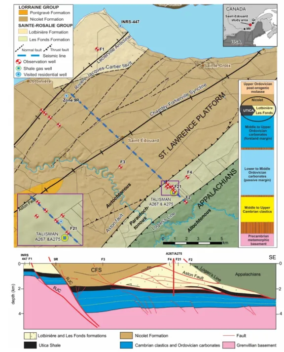
Fig. 1 Location of the study area and the monitoring wells discussed in this study (those
143
showing a name), the dashed blue line locates a seismic section, the interpretation of which
144
is shown at the bottom (from Lavoie et al., 2016). The position of monitoring wells
145
discussed in this study are projected on the geological cross-section. Inset: schematic
146
stratigraphic section of the Cambrian-Ordovician succession of the St. Lawrence Platform
147
in southern Quebec with, circled, the Upper Ordovician fine-grained clastic forming the
9
shallow bedrock of the study area (modified from Lavoie et al. 2016). Not to scale. RJC:
149
Rivière Jacques-Cartier fault, CFS: Chambly-Fortierville syncline, Mtl: Montreal, Qc:
150
Quebec City.
151 152
The detailed organic geochemistry of the shallow bedrock units of the study area has shown
153
that the shale-dominated successions have some good (Lotbinière and Les Fonds
154
formations) to low (Nicolet Formation) organic matter content and have generated and still
155
contain volatile hydrocarbons (Lavoie et al. 2016). The isotopic (δ13C and δ2H)
156
compositionof methane, ethane and propane extracted from the rock indicate a thermogenic
157
origin with increasing microbial contribution in the upper (< 50 m) and more fractured
158
intervals of the studied cores (Lavoie et al. 2016).
159
Surficial sediments in this region are usually thin (< 10 m) and made up of reworked tills
160
and near-shore sediments of the former Champlain Sea, except in a few areas where
fine-161
grained marine sediments have accumulated in local lows of the paleo-topography. When
162
thicker, these sediments usually contain coarser horizons that can be used for water supply,
163
as is the case for the municipality of Saint-Édouard.
164 165
3.2 Hydrogeological context and methane in groundwater 166
167
Groundwater in the St. Lawrence Lowlands has been known to contain high concentrations
168
of dissolved methane in certain areas since the 1950’s (Clark 1955). The Saint-Édouard
10
region was found to contain methane in groundwater almost everywhere during our
170
research project(Bordeleau et al. 2015, with measured dissolved methane concentrations
171
sometimes being above saturation under atmospheric conditions. Residential wells in this
172
area are mostly open boreholes completed into bedrock (shale) with generally unsealed
173
metal casing across surficial sediments. Residential wells have depths that generally vary
174
between 20 m and 80 m, with an average of about 50 m. This shale has a poor permeability,
175
having hydraulic conductivities between 10-9 to 10-6 m/s, and the active groundwater flow 176
zone is shallow (< 30 m within bedrock) (Ladevèze et al. 2016).
177
Methane concentrations in groundwater in the Saint-Édouard region is strongly correlated
178
to the water type, with higher concentrations (up to 80 mg/L) found in water containing
179
more sodium (NaHCO3 and NaCl types) compared to relatively less geochemically evolved 180
CaHCO3 water (Bordeleau et al. 2015). These findings are in agreement with many other 181
studies elsewhere (e.g. Molofsky et al. 2013 and 2016a; Darrah et al. 2014; LeDoux et al.
182
2016; Siegel et al. 2016), as well as over the entire St. Lawrence Lowlands (Moritz et al.
183
2015). Dissolved methane in the Saint-Édouard area was found to be of predominantly
184
microbial origin, with contribution of thermogenic methane in approximately 15% of the
185
wells (Bordeleau et al. 2017), which is also in agreement with the regional study over the
186
St. Lawrence Lowlands that found predominantly microbial methane in groundwater
187
(Moritz et al. 2015). In the study area, both types of methane were shown to come from the
188
shallow bedrock, which is mainly composed of organic-rich shales (Lavoie et al. 2016).
189
There is currently no Canadian drinking water quality guideline for dissolved methane as
190
this component is not related to a health issues. However, the Ontario drinking water
191
standards provide an aesthetic objective for methane of 3 L/m3 (i.e., 2 mg/L) to limit
11
problems with gas bubble release and spurting from taps (Kennedy and Drage 2015), while
193
the alert threshold for the province of Quebec and Pennsylvania State is 7 mg/L and for
194
Ohio State 10 mg/L, mainly to avoid risk of explosion. The U.S. Department of the Interior
195
recommends periodic monitoring when dissolved methane concentrations range between
196
10 and 28 mg/L and remedial action when concentration exceeds 28 mg/L (U.S.
197
Department of the Interior 2001).
198 199
3 Methodology
200 201
3.1 Drilling and selection of wells for the monitoring program 202
203
Fifteen observation wells were drilled into bedrock within the framework of the project, of
204
which eight were diamond-drilled in order to have core samples for various analyses (e.g.
205
Lavoie et al. 2016) and five were selected for frequent groundwater monitoring. The
206
locations of the 15 observation wells were chosen in order to achieve good spatial coverage,
207
obtain samples from the different geological formations, and collect a higher density of
208
data close to the faulted zones that could represent fluid migration pathways between the
209
deep and shallow domains. Indeed, a natural connection between deep units and surficial
210
aquifers is presumed possible only if permeable discontinuities are present, such as
211
permeable fault zones (Gassiat et al., 2013; Birdsell et al., 2015). Therefore, most of the
212
monitoring wells were drilled close to two known fault zones: the Logan’s Line – Aston
12
fault system (thrust faulting) in the southern part of the study area and the Jacques-Cartier
214
River fault (normal faulting) in the northern part (Fig. 1).
215
The seven (7) wells used for the temporal methane monitoring program reported in this
216
paper were selected based both on their spatial coverage and on their range of
217
concentrations and isotopic signatures. They included five (5) observation wells (F1, F2,
218
F3, F4 that were diamond-drilled in 2013 and F21 that was diamond-drilled in 2014), and
219
two residential wells (INRS-447 and Zone 9R) (Fig. 1). All the observation wells are open
220
to the fractured rock aquifer and a sealed metal casing was put across surficial sediments
221
and anchored in the top part of bedrock. They were developed just after completion using
222
compressed air to empty them to make sure that the water used as a drilling fluid was
223
removed before sampling. These observation wells are either under confined (wells F1, F3
224
and F4) or semi-confined (wells F2 and F21) conditions (Ladevèze et al. 2016) and their
225
general characteristics are summarized in Table 1. The confinement of the fractured rock
226
aquifer can either come from low-permeability surficial deposits or a lack of fractures in
227
the upper part of the shale unit making up the rock aquifer. More details on these wells and
228
their construction are provided in Ladevèze et al. (2016).
229
The use of residential wells in baseline studies has been discouraged by Jackson and Heagle
230
(2016), mainly due to potential surface contamination by septic tank effluent, de-icing salt
231
and agricultural residues, poor maintenance of the well and of the plumbing, as well as a
232
poor construction. However, we wanted to include both observation and residential wells
233
in the monitoring program, as their characteristics are very distinct: residential wells are
234
used continuously for domestic purposes and their construction dates back several years,
13
while our recent monitoring wells are dedicated, mostly isolated wells only pumped
236
sporadically and at a very low yield.
237 238
Table 1 Characteristics of the monitoring wells used in this study
239 Site Well type Drilling type Drilling year Total drilled depth (m bgs) Static water level (m bgs) Overburden thickness (m bgs) Sampling depth (m bgs) Geological unit F1 OW D-D 2013 50 -0.02 2.44 7.5 Lotbinière F2 OW D-D 2013 52 1.55 6.1 21.5 Les Fonds F3 OW D-D 2013 50 0.79 20.12 22.7 Nicolet F4 OW D-D 2013 60 7.51 40.84 54 Les Fonds F21 OW D-D 2014 147 4.77 4.57 145 Les Fonds
INRS-447 RW H-D 2009 12.8 1.22 9.2 At the tap Lotbinière
Zone 9R RW H-D 1967 45.7 1.22* 5.5 At the tap Nicolet
OW: Observation well drilled for the project; RW: Residential well used for water supply; D-D:
Diamond-240
drilled well with a 100 mm (4 in.) diameter; H-D: hammer-drilled well with a 152 mm (6 in.) diameter; m
241
bgs: meters below ground surface. * The only data available dates back to its drilling year (1967), as we did
242
not get the owner authorisation to open the well.
243 244
This decision to include residential wells was also based on the fact that sampling
245
residential (or irrigation) wells in a baseline study is almost inevitable, as it allows for a
246
much better coverage of a study area at a reasonable cost, compared to the drilling of costly
247
dedicated observation wells. In fact, this is typically what is done by oil and gas companies
248
to establish baseline conditions. We therefore wanted to follow both types of wells and
249
verify whether methane variations would be similar. While it is true that residential wells
250
are vulnerable to the potential issues discussed in Jackson and Heagle (2016), the water
251
geochemistry from the two residential wells selected for the temporal monitoring program
14
has been carefully examined, to ensure these wells were suitable for monitoring and that
253
their results were representative of natural groundwater. These two residential wells are
254
likely under confined or semi-confined conditions like the other wells in this study area
255
and did not appear to be contaminated by de-icing salts or other anthropogenic sources
256
based on their general geochemistry results. Another issue with residential wells is that
257
their usage could result in a significant drawdown in the well and, therefore, degassing in
258
the well. The two selected residential wells were always sampled at a low flow rate during
259
the day, while the owners were not home.
260 261
3.2 Monitoring program 262
263
Temporal geochemical monitoring began in November 2013 with the first four wells
264
drilled for the project (F1 to F4; Table 1). The two residential wells (INRS-447 and Zone
265
9R), which were first sampled in summer 2013, were added to the monitoring program the
266
next spring. The deepest observation well (F21; Table 1) was added to the program after
267
its completion in November 2014. These wells were sampled regularly (every 2 to 3
268
months), except during winter, when the frequency was lower due to accessibility and
269
freezing (when water level is close to the surface) issues such as for well F1. In the last
270
year of the project (March 2015 - February 2016), the sampling frequency was increased
271
to once a month for wells F4 and F1 (except in winter months for F1).
272
As part of the monitoring program, the collected water samples were analyzed for alkane
273
(methane, ethane, propane) concentrations and for methane isotopic composition (δ13
15
CH4, δ2H- CH4) when concentrations allowed (generally in the order of 150 µg/L of 275
methane). Relatively early in the monitoring program, dissolved inorganic carbon (DIC)
276
concentrations and its isotopic composition (δ13C-DIC) were also added, as these
277
parameters could provide important information regarding the origin of methane. To our
278
knowledge, this is the first documented record of such complete yearly geochemical
time-279
series.
280
Groundwater levels were also monitored every 15 minutes in each monitoring well with
281
pressure loggers, completed by barometric pressure measurements in three wells (F1, F2
282
and F4) (Ladevèze et al. 2016).
283 284
3.3 Groundwater sampling, storage and chemical analysis 285
286
Observation wells F1 to F4 were sampled using either a Redi-Flo2 impeller pump
287
(Grundfos, Bjerringbro, Denmark) or a Solinst (Georgetown, ON, Canada) model 407
288
bladder pump, both with 6.25 mm (¼”) diameter tubing. Observation well F21, due to its
289
greater sampling depth (145 m), had to be sampled using HydraSleeve (Las Cruces, NM,
290
USA) single-use sampling bags, a simple device consisting of a polyethylene bag sealed at
291
the bottom and with a self-sealing check valve at the top. Careful comparison of these
292
different devices will be documented in an upcoming paper; results showed that they
293
produce comparable results for concentrations and isotopic ratios.
294
Samples were always collected for a given well at the same depth (see Table 1). Packers
295
were not used to isolate a specific interval, because this technique would have been
16
extremely time consuming, and sampling five wells at such high frequency in this manner
297
would not have been practically feasible. Instead, the pump or bag was slowly and carefully
298
lowered in the well and was positioned at the depth where the most productive fracture(s)
299
had previously been identified by borehole geophysical methods (Crow and Ladeveze
300
2015), to ensure that only “fresh” groundwater from the flowing fractures was being
301
pumped. Physico-chemical profiles were carried out in four wells at 5-m intervals and the
302
distinct characteristics obtained at each interval confirmed that the sampling method was
303
appropriate for targeting water from a given depth. When pumps were used, the pumping
304
rate was kept at a minimum (well below the 500 mL/min low-yield recommended by the
305
EPA), which limited drawdown, thus preventing degassing of the water in the well. The
306
median drawdown was 59 cm for monitoring wells F1 to F4, due to the very
low-307
permeability rock. The two residential wells (INRS-447 and Zone 9R) were sampled
308
upstream from any treatment system, using 6.25 mm (¼”) diameter tubing connected to
309
the outdoor spout. Sampling was again performed at a very low yield (below the
310
recommended 500 mL/min) to minimize drawdown (average yield was 260 mL/min). It
311
was carried out during the day when the wells had not been used for a few hours. While
312
the use of an outdoor tap when the owners were not home can result in some gas loss
313
(although all sampled water tanks were pressurized), this also ensures that no domestic
314
device uses water at the time of sampling, which could cause important drawdown in the
315
well.
316
For all wells, samples for alkane concentrations and isotopic composition were collected
317
by placing the sampling bottle (40 mL glass amber vials for concentrations and 1L amber
318
glass bottles for isotopes) in a larger container, and positioning the sampling tube at the
17
bottom of the bottle, as recommended for analyses of dissolved gas by the U.S. Geological
320
Survey (http://water.usgs.gov/lab/chlorofluorocarbons/sampling/bottles/). Water filled the
321
bottle, then the larger container. The tube was slowly removed from the submerged bottle,
322
and the bottle was rapidly capped under water. This sampling procedure represents a
“semi-323
closed” system, as described by Molofsky et al. (2016b). Such a sytem provides good
324
results for low and intermediate methane concentrations (i.e. samples not supersaturated
325
with dissolved gases), but methane concentrations in gas-charged (effervescing) samples
326
are likely underestimated (Molofsky et al., 2016b). However, obtaining exact
327
concentrations was not crucial for this study, because the monitoring program was mainly
328
put in place to follow stable isotope ratios so as to identify methane origin. Nonetheless,
329
documenting the extent of methane concentration variations obtained under these typical
330
sampling conditions was also deemed valuable. The pH in the samples was lowered to <2
331
using hydrochloric acid to prevent microbial activity, and the bottles were kept refrigerated
332
either upside down or on their side. Samples for δ13C-DIC were collected by simply filling 333
the 40 mL amber glass vials completely (without air) with filtered groundwater (using a
334
0.45 µm nylon membrane). These samples were not acidified, as this would have caused
335
degassing of CO2. 336
Concentrations of alkanes were determined at the Delta-Lab of the Geological Survey of
337
Canada (Quebec City, QC, Canada) using a Stratum PTC (Teledyne Tekmar, Mason, OH,
338
USA) purge and trap concentrator system interfaced with an Agilent (Santa Clara, CA,
339
USA) 7890 gas chromatograph equipped with a flame ionisation detector (GC-FID).
340
Quantification limits on the samples were 0.006, 0.002, and 0.01 mg/L for methane, ethane
341
and propane, respectively. Methane carbon and hydrogen stable isotope ratios were
18
analyzed at the Delta-Lab, at the G.G. Hatch laboratory of the University of Ottawa (ON,
343
Canada) or at Concordia University (Montreal, QC, Canada) using gas chromatographs
344
interfaced with isotope ratio mass spectrometers (GC-IRMS). The methane in some
345
samples was analyzed in duplicate at the three labs to ensure that results were comparable.
346
Details concerning the analytical procedures and quality control at each lab are found in
347
Appendix A5. Results are expressed in the usual per mil notation relative to Vienna Pee
348
Dee Belemnite (VPDB, for δ13C) and Vienna Standard Mean Ocean Water (VSMOW, for 349
δ2H). Precision is typically ≤ 0.5‰ for δ13C and ≤ 3.0‰ for δ2H. Finally, analyses for δ13 C-350
DIC were done at the University of Waterloo (ON, Canada) using a MicroGas-IsoPrime
351
(Manchester, UK) mass spectrometer, and results are expressed with respect to VPDB.
352
Precision is ± 0.2‰.
353 354
3.4 Estimation of uncertainty related to sampling, handling and analytical procedures 355
356
The uncertainty due to sampling, handling and analytical procedures was evaluated for
357
alkane concentrations and methane C and H isotopes, using replicate samples collected
358
within the framework of the larger Saint-Édouard project. For concentrations, 55 samples
359
were collected and analyzed in triplicate. For each sample, the three bottles were collected
360
within a few seconds of one another in the field, under the same conditions and in the same
361
larger container, and were analyzed (one analysis each) sequentially. Methane
362
concentrations in the 165 bottles (55 samples x 3 bottles) varied between 0.15 and 57.2
363
mg/L. For convenience of comparison with other papers, the uncertainty was assessed
19
through two common approaches, i.e. using either the relative error ([Cmax-Cmin]/Cmax) or 365
the coefficient of variation (CV= standard deviation / mean). Relative errors and CVs were
366
used to remove the dependence of uncertainty on absolute concentrations. Indeed, methane
367
concentrations in our samples vary over nearly three orders of magnitude, and so does the
368
absolute uncertainty; hence, the use of relative values provides one criteria that is
369
applicable to all samples. For both approaches, descriptive statistics are presented in Table
370
A1 in Appendix A2. This table includes the minimum, maximum, median, and 90th 371
percentile values, all expressed in percent (%). Although estimated with only three values
372
each time, CVs provide an order of magnitude of the uncertainty that is useful for later
373
comparaison with monitored concentrations (in section 4). The statistics selected to
374
represent the uncertainty on all the methane concentration values in this research project is
375
the 90th percentile value of the coefficient of variation and is 15% in this case. 376
The approach used to estimate uncertainty on isotope ratios was slightly different, mainly
377
due to the higher analytical costs, and to the larger volume of water that needs to be
378
collected, handled and stored (3 x 40 mL bottle for concentrations versus 2 x 1L bottle for
379
isotope ratios). For the isotope ratios, an absolute uncertainty value may be reasonably
380
estimated, because the variations in magnitude between the isotopic ratios of individual
381
samples are actually very small; hence, the uncertainty is not very much affected by
382
individual sample results. Standard deviation is therefore used for convenience of
383
expressing uncertainty in per mil (‰) (Table A1). For methane carbon and hydrogen stable
384
isotope ratios, 15 samples were collected in duplicate in the field. The selected statistics
385
for methane isotopes is the 90th percentile value of the standard deviation rounded off to 386
20
the nearest integer, which is 1.7‰ for carbon isotopes (δ13C) and 19‰ for hydrogen
387
isotopes (δ2H). 388
389
4 Results and related discussion
390 391
Results obtained for residential wells are considered separately from those for observation
392
wells, since residential wells are used on a daily basis and could be subject to different
393
conditions affecting the concentrations and isotopic composition of methane (see Section
394
3.1). All geochemical results will be available in a public database to be released in 2017,
395
excluding name and address of well owners, as well as the geographical coordinates of
396
residential wells.
397 398
4.1 Concentrations of methane and higher alkanes 399
400
Concentrations measured in the selected monitoring wells are representative of the region,
401
and temporal variations of these concentrations are shown in Figures 2 and 3. For the two
402
residential wells, methane concentrations data go from summer 2013 to winter 2016,
403
whereas values for the observation wells either begin in the fall of 2013 (F1 to F4) or 2014
404
(F21) depending on their completion date. Values for methane concentrations were
405
classified either as “low” (detection limit to 1 mg/L), “intermediate” (1 to 7 mg/L, the latter
21
corresponding to the alert threshold for the Quebec Department of Environment), or “high”
407
(> 7 mg/L).
408
409
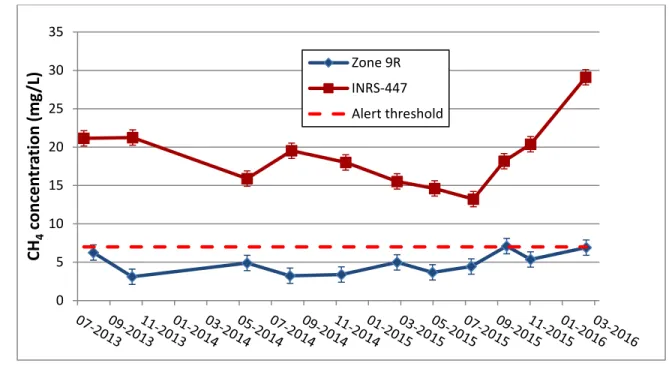
Fig. 2 Methane concentrations over time for the two residential wells. Uncertainty,
410
represented by error bars, is ±15% of the values. The alert threshold for the Department
411
of Environment of Quebec (7 mg/L) is shown using a dashed red line. Note: These two
412
wells were sampled the first two times using a 19 mm (¾’’) garden hose, then using a
413
6.25 mm (¼’’) hose, which may have led to an underestimation for well INRS-447 as
414
concentrations are high.
415 416
Water from both residential wells is of the geochemically evolved Na-HCO3 type and 417
contains hydrogen sulfide, with the accompanying typical strong “rotten egg” odor. Well
418
Zone 9R, constructed in 1967, is located along the Jacques-Cartier River fault in an area
419
underlain by the organic-lean Nicolet Formation (Lavoie et al. 2016) (Table 1 and Fig. 1).
420 0 5 10 15 20 25 30 35 CH4 con ce nt ra tion (m g/ L) Zone 9RINRS-447 Alert threshold
22
Well Zone 9R exhibits “intermediate” methane concentrations, varying between 3.1 and
421
7.1 mg/L, with a CV of 52% and a maximum over minimum (max/min) concentration ratio
422
of 2.29. Noteworthy, while ethane has never been detected in samples from this well,
423
propane was present in the first sample (350 μg/L), but was never detected in subsequent
424
samples. One factor that differs between the first sampling event and the following ones is
425
the duration of pumping before sampling, which was much longer at the first visit (about
426
90 minutes compared to 20 minutes for the subsequent visits). This well is not very
427
productive and, due to water shortage resulting from our first visit, the owner required that
428
we pump for a shorter period of time in the future. However, as this well is regularly used
429
for domestic needs, the physico-chemical parameters have always reached stability within
430
this 20-min period. It is inferred that the longer pumping time during the first sampling
431
event had drawn in water from different, lower strata, where thermogenic gas (containing
432
propane) is present.
433
Well INRS-447, constructed in 2009, is located within a few tens of meters of the St.
434
Lawrence River in an area underlain by the Lotbinière Formation, which is hydrocarbon
435
volatiles-rich (Lavoie et al. 2016) (Table 1 and Fig. 1). In residential well INRS-447,
436
methane concentrations are high and variations in the absolute concentrations are greater
437
than for the previous well, with observed measured concentrations between 13.2 and 29.1
438
mg/L. However, the relative variation is lower, with a CV of 25% and a max/min
439
concentration ratio of 2.20. Methane concentrations in this well gradually decreased during
440
the first 2 years (from 21 mg/L to 13 mg/L). Nonetheless, a marked increase is observed in
441
the last three sampling campaigns (Fig. 2), similarly to most observation wells (see below).
442
Groundwater consistently contained ethane and propane, with median concentrations of 96
23
and 78 μg/L, respectively. In all but one sample from this well, the proportions of methane
444
to ethane + propane (dryness ratio) varied between 103 and 656, pointing towards mixed
445
thermogenic and microbial gas origin (results of dryness ratios over time are provided in
446
section A3 of the Appendix).
447
Observation wells F1, F2, F4 and F21 have “high” (>7 mg/l) methane concentrations, while
448
well F3 generally has “low” (detection limit to 1 mg/l) concentrations. As for the residential
449
wells, high concentrations are found in wells drilled in the hydrocarbon volatiles-rich
450
Lotbinière and Les Fonds formations (i.e. wells F1, F2, F4 and F21, see Table 1 and Fig.
451
1). For all wells, concentrations vary considerably over time, with CV of 34% for F1, 57%
452
for F2, 236% for F3 (although large in percentage due to the first higher value, absolute
453
changes in concentration were not major for this low concentration well; see Figure 3),
454
22% for F4 (54 m depth), and 45% for F21. The temporal variation in each well is therefore
455
higher than the combined uncertainty introduced by sampling, handling and analytical
456
procedures, which is 15% (see section 3.4).
24 458
Fig. 3 Dissolved methane concentrations over time for the five observation wells.
459
Uncertainty, represented by error bars, is ±15% of the values. Notes: 1) the first two
460
values for wells F2, F3 and F4 were obtained using an impeller (Redi-Flo2) pump that
461
had a 19 mm (3/4’’) tubing, which may have lead to more degassing and thus
462
underestimated methane concentrations; 2) well F4 was initially pumped at a depth of 30
463
m, before a 90-m impeller pump was available.
464 465
For well F3 (drilled in the Nicolet Formation), the first value obtained a few days after
466
drilling was 11 mg/L. Concentrations rapidly dropped in the following months and have
467
remained between 0.1 and 1 mg/L for the last two years. This is likely due to the fact that
468
some of the methane contained in the rock surrounding the borehole was rapidly released
469
during and after drilling, while the free-flowing groundwater contains very little methane.
470 0 10 20 30 40 50 60 70 80 90 100 CH 4 con ce nt ra tion (m g/ L) F1 F2 F3 F4 (54 m) F21 F4 (30 m) Alert threshold
25
A somewhat similar situation occurred at well F1 (in the Lotbinière Formation), which was
471
visibly degassing just after drilling, with audible bubbling and fumes coming out of the
472
well, which stopped a few weeks later. In this well, methane, ethane and propane
473
concentrations were highest a few weeks after drilling (39.0, 4.8 and 3.4 mg/L,
474
respectively) and then declined during the first year. However, methane concentrations
475
started to rise the second year to eventually reach values similar to the one obtained during
476
the first sampling campaign, but this was not the case with ethane and propane. It is
477
therefore likely that the thermogenic gas present in the rock was released shortly after
478
drilling, being then replaced by mixed gas (with a higher proportion of microbial gas) found
479
in groundwater. The dryness ratio of 10 obtained in the first sample was the lowest of the
480
series, but the subsequent ratios remained quite low (between 44 and 247), within the
481
thermogenic or mixed gas domains (see Appendix A3). Only two samples from F1 had no
482
detectable ethane or propane, indicating a strong predominance of microbial gas at that
483
time (confirmed by isotopic ratios, see below).
484
For well F4 (in the Les Fonds Formation), the first value of five obtained at the 30 m depth
485
was also the highest concentration recorded at this depth. The same early degassing
486
situation as for F1 and F3 is thus suspected, although it is difficult to draw a firm conclusion
487
since the following concentrations were obtained at greater depth (Fig. 3). The
488
concentration at a 30 m depth appears to be approximately half of that at 54 m based on
489
the two sets of samples taken the same day, confirming that sampling must always be done
490
at the same depth within a timeseries in order to have comparable data.
491
In wells F2 and F21 (also in the Les Fonds Formation), early degassing is not suspected,
492
as the concentrations in the first samples are not the highest of the series. Well F2 contains
26
microbial gas (based on the very low ethane and propane concentrations, and on isotopic
494
ratios of methane, see below), while well F21 consistently contained ethane and propane,
495
with dryness ratios varying between 27 and 46, indicating the presence of thermogenic gas.
496
In four of the five observation wells, the max/min methane concentration ratios are
497
somewhat similar (2.54 for F1, 6.26 for F2, 2.87 for F4, 3.47 for F21), and resemble the
498
ratios in residential wells. In contrast, the max/min ratio is much higher for well F3 (>58),
499
because the first two values (and especially the first one) from this well were much higher
500
than the subsequent ones (this ratio drops to 5.2 when rejecting the first two values). In
501
most of our monitoring wells (except F3 and Zone 9R), an increase in methane
502
concentration was observed during the second year of sampling. In observation wells, the
503
increase generally began in November 2014, while the rise for the residential well
INRS-504
447 started only in July 2015. Because the project ended in March 2016, we do not know
505
whether the concentrations would have continued to increase, thus increasing the max/min
506
ratios.
507
Ethane concentrations were above a few μg/L only in three wells (INRS-447, F1 and F21;
508
all in the volatiles-rich Lotbinière and Les Fonds formations); they showed a quite good
509
coefficient of correlation with methane concentrations (R2=0.77). Propane in groundwater 510
was present in significant concentrations over time only in well F21, and the seven data
511
available showed a weak coefficient of correlation with methane (R2=0.30). Dryness ratio
512
values over time for the 7 observation wells are presented in Appendix (section A3). They
513
also show highly variable values, except for well F21 that has relatively stable ratios mainly
514
due to the quite good correlation between methane and ethane concentrations.
27 In an attempt to explain the temporal variation for methane concentrations in the different 516
wells, total precipitation and water level (corrected for barometric pressure changes) time-517
series were plotted against available methane concentrations. Comparisons were made 518
using daily, weekly and monthly precipitation and water-level data (not shown). Methane 519
concentrations do not appear to be strongly related to precipitation or groundwater levels, 520
either seasonally or over the whole period. Methane concentrations in a well (and even 521
more so in a collected water sample) depend on multiple factors, and recharge is a complex 522
process resulting from all the other water budget components. Hence, it does not appear 523
possible for methane concentrations to be predicted using parameters such as precipitation 524
and water levels, at least in the study area. It is expected that other regions that share a 525
similar hydrogeological context with high concentrations of dissolved methane in shallow 526
low-permeability aquifer would behave similarly (e.g., in Pennsylvania and West Virginia 527
as described in Sharma et al. 2013, Molofsky et al. 2013; Siegel et al. 2015). 528
529
4.2 Methane isotopic composition 530
531
The main interest of this study was to investigate whether methane carbon and hydrogen
532
stable isotope ratios varied over time, as do methane concentrations (Figures 4 and 5). In
533
most samples, carbon stable isotope ratios (δ13C-CH4) are between -70 and -50‰, and are 534
therefore somewhat close to the boundary between the typical isotopic domains defined for
535
thermogenic gas (> -50‰) and microbial gas (usually < -60‰, but sometimes heavier, i.e.
536
between -50 and -60‰, when originating from acetate fermentation or when subjected to
28
post-genetic transformation processes), as suggested by several authors (e.g. Whiticar
538
1999; Golding et al. 2013). Such intermediate values can be the result of mixing between
539
gas of different origins, or alterations of microbial gas through processes that increase the
540
δ13C value, such as partial methane oxidation or methane generation from an old, partially 541
exhausted carbon reservoir (late-stage methanogenesis) (Bordeleau et al. 2015). An
in-542
depth study of the origin of the methane found in the different wells of the study area will
543
be the subject of an upcoming paper.
544
Figure 4 shows that residential well INRS-447, which has high methane concentrations
545
(Fig. 2), exhibits δ13C values steadily around -60‰, with a standard deviation (SD) of
546
1.5‰. Its variations throughout the timeseries are therefore within the variations expected
547
from sampling, handling and analysis (1.7‰ for SD see Table A). As mentioned in section
548
4.1, samples from this well consistently contained ethane and propane, with resulting
549
dryness ratios being in the mixed thermogenic/microbial domain (see Figure A1 in
550
Appendix A3). In this case, mixing between both sources appears to be rather uniform in
551
parts of the aquifer penetrated by the well, which results in relatively constant δ13C values
552
obtained in the timeseries.
553
In contrast, in residential well Zone 9R, which contains intermediate methane
554
concentrations, the first sample has a significantly higher δ13C ratio (-43.5‰) compared to
555
subsequent samples (Fig. 4a); it was also the only sample from this well to contain propane.
556
All subsequent δ13C values obtained from this well were within the microbial domain (-557
61.3 to -76.6‰), but varied more than in well INRS-447 (SD of 8.0‰ when including the
558
first sample, and SD of 4.0‰ when excluding it). The variations in the timeseries therefore
559
exceed the uncertainty related to sampling, handling and analysis. The isotopic values in
29
well Zone 9R support our earlier hypothesis that the longer pumping time and higher
561
pumping rate exerted during the first sampling event drew in water from different strata
562
containing thermogenic gas. Therefore for this well, it seems possible to obtain gas from
563
different origins, but the proportions are not stable and rather depend on pumping duration
564
and the related drawdown.
565
In observation wells F1, F2, F4 (30 m and 54 m) and F21, variations of δ13C are also limited
566
(Fig. 4b), with SDs ≤ 2.2‰. Variations are therefore somewhat comparable to residential
567
well INRS-447, and generally lie within the uncertainty expected for sampling, handling
568
and analysis. In well F3, lower δ13Cvalues (-95 to -63‰) compared to those of the other
569
wells were found, and variations are much more important, with a SD of 10.8‰. In this
570
well, ethane and propane were never detected, but this may only be due to the fact that
571
methane concentrations are very low (generally below 1 mg/L), so a mixed gas origin
572
cannot be excluded. However, even if the gas is entirely microbial, due to the low methane
573
concentrations, processes affecting the methane (e.g. oxidation), even if occurring to a
574
limited extent, could have a pronounced effect on the isotopic ratios (see below).
30 576
577
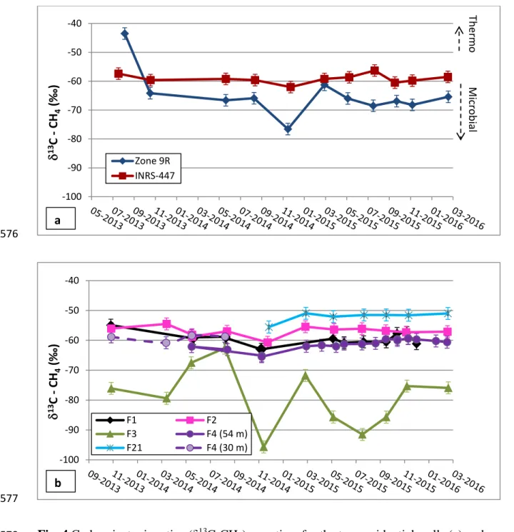
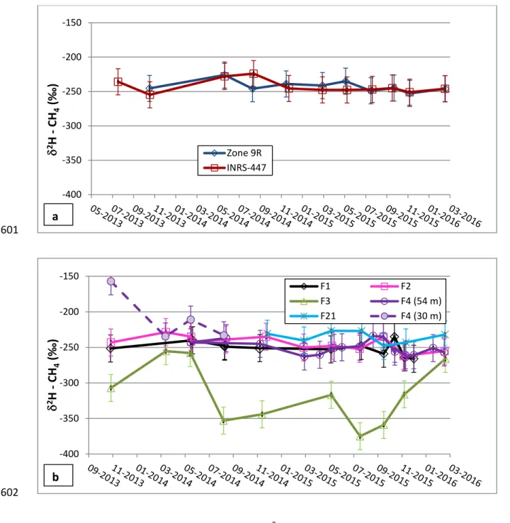
Fig. 4 Carbon isotopic ratios (δ13C-CH4) over time for the two residential wells (a) and 578
the five observation wells (b). Uncertainty, represented by error bars, is ±1.7‰. Note:
579 Thermo: thermogenic. 580 581 -100 -90 -80 -70 -60 -50 -40 δ 13 C -CH 4 (‰ ) Zone 9R INRS-447 -100 -90 -80 -70 -60 -50 -40 δ 13 C -CH 4 (‰ ) F1 F2 F3 F4 (54 m) F21 F4 (30 m) M ic ro bial a b Th er m o
31
Hydrogen stable isotopic values (δ2H) were also monitored over time. These values are
582
normally more variable than δ13C (Whiticar 1999; Golding et al. 2013) and there is 583
considerable overlap between the hydrogen isotopic domains defined for microbial and
584
thermogenic gas. The δ2H values must always be used together with δ13C values in order 585
to provide useful information concerning the origin of methane, because methane of
586
thermogenic and microbial origins would not necessarily have distinct δ2H values.
587
However, if processes such as oxidation affected methane in groundwater, the isotopic
588
effect would be more pronounced on hydrogen isotopes than on carbon isotopes (Alperin
589
et al. 1988; Grossman et al. 2002; Kinnaman et al. 2007).
590
In most of the wells, δ2H values were remarkably stable over time (Fig. 5). In residential
591
wells, the SDs are 7.7‰ for Zone 9R (excluding the first sample of the series, as there was
592
no δ2H value available for this sample) and 9.6‰ for INRS-447. Similar results were 593
obtained for observation wells F1, F2, F4 (54 m) and F21, with SDs ≤ 11.5‰. An exception
594
is well F4 (30 m depth), which had a surprisingly high δ2H value of -157‰ in the first
595
sample. No explanation has been found for this first value, as there does not seem to be a
596
mixing between microbial and thermogenic gas sources (no ethane or propane were
597
detected) and oxidation does not seem plausible (the carbon isotopic ratio in the first
598
sample is not different from subsequent samples).
599 600
32 601
602
Fig. 5 Values of methane hydrogen isotope (δ2H-CH
4) over time for the two residential 603
wells (a) and the five monitoring wells (b). Uncertainty, represented by error bars, is
604 ±19‰. 605 606 -400 -350 -300 -250 -200 -150 δ 2H -CH 4 (‰ ) Zone 9R INRS-447 -400 -350 -300 -250 -200 -150 δ 2H -CH 4 (‰ ) F1 F2 F3 F4 (54 m) F21 F4 (30 m) b a
33
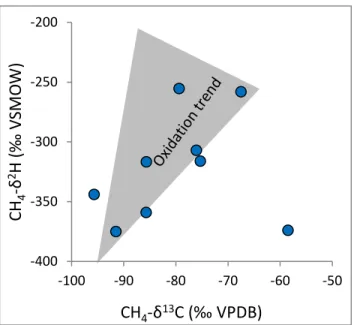
In well F3, as for δ13C values, the δ2H values are lower (between -375 and -255‰) and 607
more variable than in the other wells, spanning an impressive range of 120‰, with a SD
608
of 46.1‰. This suggests that methane may have been partially oxidized in this well and
609
because concentrations are low, the isotopic effect is readily perceptible. To evaluate this
610
hypothesis, we considered fractionation factors (α) documented by various authors
611
(Alperin et al. 1988 and authors therein; Kinnaman et al. 2007; Grossman et al. 2002),
612
which vary between 1.005 and 1.031 for carbon, and between 1.103 and 1.325 for
613
hydrogen. An original (non-oxidized) isotopic ratio of -95‰ was selected for carbon and
614
of -400‰ for hydrogen, based on the results of one of the F3 samples obtained with
615
HydraSleeve bags (thus not shown in Figures 4 and 5): δ13C = -95‰ and δ2H=-393‰ for 616
a methane concentration of 0.48 mg/L. These values, although extremely low, are
617
nonetheless within the range of uncertainty of the loest values shown in Figure 5b. The
618
range of δ13C versus δ2H values that could result from progressive methane oxidation was 619
calculated using the afore-mentioned fractionation factors (shown as a grey area in Fig. 6).
620
Most of the data points from well F3 do fit within this range (see Fig. 6), in support of the
621
oxidation hypothesis, to explain the highly variable isotopic ratios measured in this well.
34 623
Fig. 6 Isotopic values (δ13C and δ2H) for methane in well F3 (circles) and range of
624
isotopic values that could result from progressive methane oxidation (grey area).
625 626
Figures 4 and 5 reveal that wells from this study area that have high methane concentrations
627
(>7mg/L) generally have stable carbon and hydrogen isotope ratios with variations within
628
the expected uncertainty arising from sampling, handling and analysis. However, wells that
629
have low or intermediate methane concentrations (such as F3 and Zone 9R) appear to have
630
carbon and hydrogen stable isotopic values that vary more importantly over time, being
631
influenced either by mixing of two gas sources in varying proportions or by partial methane
632
oxidation. Because wells Zone 9R and F3 have lower methane concentrations than other
633
wells in the monitoring program, any process affecting methane would have an impact on
634
both stable isotope ratios that is more significant than in other wells, as long as these
635
processes involve a change in isotopic ratios (i.e. mixing of groundwater sources that have
636
distinct isotopic signatures or post-genetic processes that cause isotopic fractionation).
637 -400 -350 -300 -250 -200 -100 -90 -80 -70 -60 -50 CH4 -δ 2 H (‰ V SM O W ) CH4-δ13C (‰ VPDB)
35 638
4.3 Dissolved inorganic carbon isotope ratios (δ13C-DIC)
639 640
The δ13C-DICvalues were also monitored over time, mainly to provide additional
641
information on methane origin within the framework of the larger project. DIC is mainly
642
composed of two major species: CO2, mostly from decaying modern organic matter and 643
HCO3-, predominantly deriving from carbonate rock dissolution (Sharma and Baggett 644
2011). The soil CO2 derived from plant decay typically has δ13C values ranging from -23 645
to -27‰ under temperate climates where C3 plants (most common in cool, wet climates)
646
are dominant (Clark and Fritz 1997; Sharma et al. 2013). As CO2-laden water percolates 647
through the soil profile, it can dissolve carbonate minerals which typically have an original
648
δ13C value very close to 0 ± 2‰ when, as in our case, carbonates were formed in a marine 649
environment (Sharma et al. 2013). This creates a mixing model whose boundaries should
650
be the carbon stable isotope ratios of the two distinct DIC sources. In fact, DIC in most
651
groundwaters circulating in Lower Paleozoic or older rocks (i.e. before the advent of
652
terrestrial plants and associated terrestrial carbonates) is made up of similar proportions of
653
both end members and have a δ13C value ranging between -11 and -16‰ (Sharma et al.
654
2013). However, positive values of δ13C-DIC may be encountered when microbial
655
methanogenesis significantly affects the DIC pool in an aquifer. Indeed, due to preferential
656
use of 12C by methanogens (Sharma and Baggett 2011), the two major documented
657
methanogenic pathways (acetate fermentation and CO2 reduction, which are both 658
composed of several reaction steps) progressively increase the δ13C value of the associated
659
DIC pool (Whiticar 1999; Martini et al., 2003; Sharma et al., 2013).
36
At the onset of methanogenesis, when the DIC pool is large compared to the amount of
661
methane produced, isotopic effects (i.e., food preference of microbes) might not be
662
perceptible. The same is true if methanogenesis occurs in an open groundwater system
663
where fresh, isotopically-light DIC is being added at a sufficient rate. In contrast, an
664
important 13C–DIC enrichement will be particularly significant in old, hydraulically
665
isolated groundwater systems where the extent of methanogenesis is important, and where
666
the DIC pool is not being replenished by regular input of fresh, isotopically-lighter DIC
667
(Whiticar 1999). While low δ13C–DIC values do not exclude methanogenesis, values above
668
+2 or +3‰ are a good indication of its occurrence, while values above +10‰ constitute an
669
unequivocal indication (Sharma et al. 2013). A significant increase in δ13C–DIC values in
670
a well where such values are normally stable could indicate some replenishment from a
671
deeper source of methane. Of note, groundwater with very high values of δ13C-DIC may 672
contain both microbial and thermogenic methane (well F21 is a good example, see below).
673
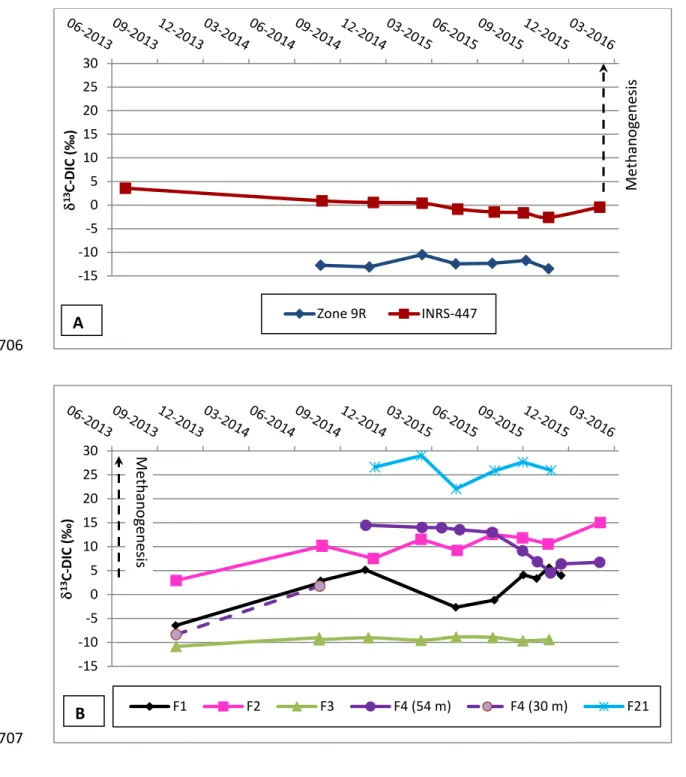
Figure 7a shows that residential well Zone 9R has stable and more typical δ13C-DIC values
674
for groundwater according to Sharma et al. (2013), varying between -10.5 and -13.5‰.
675
Except for the first sample, methane from this well is solely of microbial origin, and the
676
fact that methane does not show high δ13C-DIC values simply indicates that either: 1) the 677
carbon pool from which it is produced is being replenished by fresh carbon or 2) the carbon
678
pool is large and methane production is comparatively limited, such that the effect of
679
methanogenesis is not apparent on the δ13C-DIC values. In fact, Zone 9R is one of the two
680
wells with the highest concentration ratios of DIC/methane (between 17 and 28),
681
confirming that the carbon pool is important compared to the methane production.
682
Moreover, tritium analyses, which were conducted for the larger project, have shown that
37
there is an important modern component in the water from this well (8.2 tritium units, or
684
TU, see Table A2 in Appendix A4), indicating that there is likely some input of fresh
685
carbon in the aquifer. In the first sample collected from this well, a thermogenic gas
686
component was measured (δ13C-CH
4 of -43.5‰), but unfortunately no δ13C-DIC value is 687
available for this sample. However, the presence of thermogenic gas in this first sample
688
would not necessarily have altered the δ13C-DIC value.
689
The other residential well, INRS-447, consistently contained gas of a mixed thermogenic
690
and microbial origin. It has a comparatively higher δ13C-DIC values compared to well Zone
691
9R, varying between -2.6 and +3.6‰ (Fig. 7a). This may be due to the fact that the
692
DIC/methane ratios (between 6 and 13) are smaller than in Zone 9R and, hence, the isotopic
693
effects of methogenesis in well INRS-447 may be more visible on the DIC pool. Moreover,
694
the modern component of groundwater appears to be slightly less important (tritium result
695
of 5.7 TU, see Table A2), which suggests that the input of fresh carbon might be somewhat
696
more limited.
697
Among the observation wells, F3 is the only one with stable δ13C-DIC values that are close
698
to theoretical values for groundwater flowing into Lower Paleozoic aquifers, varying
699
between -9 and -11‰ (Fig. 7b). Methane concentrations in this well are low and the
700
DIC/methane ratio is the highest of all monitoring wells, being between 25 and 140, except
701
in the first sample where it was lower (5.8) due to the suspected early degassing of the
702
surrounding rock after drilling of the borehole. The low methane concentrations in
703
groundwater (especially compared to DIC) are not causing visible isotopic effects on the
704
DIC pool, although the methane is probably of microbial origin.
38 706
707
Fig. 7 Values of δ13C-DIC over time for residential wells (a) and observation wells (b)
708 709 710 -15 -10 -5 0 5 10 15 20 25 30 δ 13 C-DI C ( ‰ ) Zone 9R INRS-447 -15 -10 -5 0 5 10 15 20 25 30 δ 13 C-DI C ( ‰ ) F1 F2 F3 F4 (54 m) F4 (30 m) F21 M eth an og en es is M eth an og en es is A B
39
The other observation wells have higher δ13C-DIC values and more pronounced variations
711
over time (Fig. 7b). Wells F2 and F4, containing essentially microbial gas, have δ13C-DIC 712
values varying between +3 and +15‰, with half of the values being above +10‰,
713
suggesting strong microbial activity. The methane concentrations in these wells are high,
714
and DIC/methane concentration ratios are relatively low, varying between 1 and 10. Their
715
tritium content is lower than in the residential wells, with 3.8 and 1.3 TU in F2 and F4,
716
respectively (Table A2). This indicates that input of fresh carbon might be very limited in
717
these wells. Hence, the important methanogenic activity combined to isolated groundwater
718
conditions for these wells likely explains why the effect of methanogenesis is so significant
719
on the isotopic values of the DIC pool.
720
In contrast, wells F1 and F21 contain a mix of thermogenic and microbial gas, either in
721
varying (F1) or more stable (F21) proportions over time. In F1, the magnitude of variations
722
in δ13C-DIC values is similar to wells F2 and F4; however the values themselves tend to
723
be more depleted, being between -6.5 and +5.6‰ (see Figures 7b and 8a). In this case, the
724
variations appear to be related to the proportions of thermogenic and microbial gas in the
725
samples, as reflected by the relationship between dryness ratio and δ13C-DIC values (Fig.
726
8a). Samples with more microbial gas in the well F1 time-series have a higher dryness ratio
727
(less ethane and propane), lower δ13C-CH4 ratios and higher δ13C-DIC ratios. 728
40 729
730
Fig. 8 Carbon isotopic values of methane (CH4) and dissolved inorganic carbon (DIC) as 731
a function of dryness ratio, for wells F1 (a) and F21 (b).
732 733
Such correlation is not observed for well F21, which has stable dryness ratios and fairly
734
constant δ13C-CH4, but with more variable and overall higher δ13C-DIC compared to F1 735 -10 -5 0 5 -65 -60 -55 -50 0 100 200 300 δ 13 C-DI C (‰ ) δ 13 C-CH4 (‰ ) Dryness ratio (C1/(C2+C3)) Well F1, CH4 Well F1, DIC
20 25 30 35 -65 -60 -55 -50 0 100 200 300 δ 13 C-DI C (‰ ) δ 13 C-CH4 (‰ ) Dryness ratio (C1/(C2+C3)) Well F21, CH4 Well F21, DIC
b a