Morphometric, network and landscape predictors for carbon species in boreal lakes

UNIVERSITE DU QUÉBEC À MONTRÉAL

MORPHOMETRIC, NETWORK AND LANDSCAPE PREDICTORS FOR CARBON SPECIES IN BOREAL LAKES

MASTERS DEGREE THESlS IN

BlOLOGICAL SCIENCES

BY

JULIA JAKOBSSON

UNIVERSITÉ DU QUÉBEC À MONTRÉAL Service des bibliothèques

Avertissement

La diffusion de ce mémoire se fait dans le respect des droits de son auteur, qui a signé le formulaire Autorisation de reproduire et de diffuser un travail de recherche de cycles supérieurs (SDU-522 - Rév.0?-2011 ). Cette autorisation stipule que «conformément à l'article 11 du Règlement no 8 des études de cycles supérieurs, [l'auteur] concède à l'Université du Québec à Montréal une licence non exclusive d'utilisation et de publication de la totalité ou d'une partie importante de [son] travail de recherche pour des fins pédagogiques et non commerciales. Plus précisément, [l'auteur] autorise l'Université du Québec à Montréal à reproduire, diffuser, prêter, distribuer ou vendre des copies de [son] travail de recherche à des fins non commerciales sur quelque support que ce soit, y compris l'Internet. Cette licence et cette autorisation n'entraînent pas une renonciation de [la] part [de l'auteur] à [ses] droits moraux ni à [ses] droits de propriété intellectuelle. Sauf entente contraire, [l'auteur] conserve la liberté de diffuser et de commercialiser ou non ce travail dont [il] possède un exemplaire.»

UNIVERSITÉ DU QUÉBEC

À

MONTRÉAL

PRÉDICTION DES FORMES DE CARBONE DANS LES LACS

BORÉAUX,

À PARTIR DE LA MORPHOMÉTRIE, LE RÉSEAU

HYDROGRAPHIQUE ET LA STRUCTURE DU PAYSAGE

MÉMOIRE

PRÉSENTÉ

COMME EXIGENCE PARTIELLE

DE LA MAITRISE EN BIOLOGIE

PAR

JULIA JAKOBSSON

ACKNOWLEDGEMENTS

I am very grateful for the support from NSERC's CREA TE training program in lake and fluvial ecology (ÉcoLac), the Group for Interuniversity Research in Limnology and aquatic environment (GRIL), the Industrial Research Chair in Carbon Biogeochemistry in Boreal Aquatic systems (CarBBAS), my supervisors Paul del Giorgio and Yves T. Prairie, and everyone who has been involved in the sampling campaigns the last decade for making these two years of research possible.

Thanks to Richard Vogt, Tonya DelSontro and Joan Pere Casas for encouragement and improving my writing, and to Roy Nahas for bouncing GIS ideas with me. Thanks to ali colleagues in the research group: Ryan Hutchins, Marie Gerardin, Km·elle Desrosiers, Cynthia Soued, Mm1in Demers, Shoji Tottahill, Patricia Pernic, Felipe Rust, Paula Reis, Ji-Hyeon Kim, Tristy Yick-Majors, Sophie Crevceur, Sara Mercier-Blais, Alex Ducharme, Alice Parkes and Annick St-Pierre; without your invaluable feedback, laughs, chats and shared knowledge, Montreal would have been a much colder place. Also thanks to Sandro, Ariel, Lulu and Amir.

Ill Table of Contents ACKNOWLEDGEMENT ... 1 LI T OF FIGURE ... v LI T OF TABLES ... xi LIST OF ABREVATIONS ... xv

RÉ UMÉ SCIENTIFIQUE ... xvii SCIENTIFIC SUMMARY ... xix fNTRODUCTION ... 1

CHAPTER 1 ... 7

LAKE MORPHOLOGICAL REGlO S ACROS TEMPERA TE, BOREAL A D SUBARCTIC LANDSCAPES ... 7

1.1 INTRODUCTION ... 7

1.2 METI-IODS ... 12 1.3 RESUL TS ... 18 1.4 DISCUSSION ... : ... 39

1.5 CONCLUSIONS ... 44

CI-IAPTER 2 ... 47

CARBON PECIES fN RELATION TO LAKE MORPHOLOGICAL AND AQUATIC NETWORK METRICS fN BOREAL QUÉBEC ... .47

2.1 INTRODUCTION ... 47 2.2 METHODS ... 52 2.3 RESULTS ... 57 2.4 DISCUSSION ... 69 2.5 CONCLUSIONS ... 74 REFERE CES ... 77 APPENDIX ... 91 1. GIS FLOWCHARTS ... 91 11. xample images of lake cl as es ... 94

v

LIST OF FIGURES

Figure 1.2.4. An illustrated example of the transition from lake polygons to composite image. The 1 st step accounts for the calculations made from the lake polygons; the 2nd have had the lake shapes replaced with their center point; the yd have had Thies en polygons outlined; the 4th is a representation of the conversion from polygon to raster format; the 5th is the composite image of the three raster layers which will be the input to the classification ... 16 Figure 1.2.4.2 An illustrated example of the transition from an RGB-composite image of 3 PCA axes representing the red, blue and green, to an ISO cluster classification and finally a processed maximum likelihood classification ... 18 Figure 1.3.1.a-i Distribution of 9 morphometric parameters for lakes with between 0.005-1,370 km2 surface area in Québec. Ali distributions are on a logl 0 scale ... 21 Figure 1.3.2.1 Allometry regressions between ali metrics and Arca. a) Perimeter (R2=0.92), b) Maximum Depth (R2=0.1 5), c) Mean Depth (R2=0.1 5), d) Volume (R2=0.79), e) Edge Complexity (R2=0.36), t) Shape (R2=0.09), g) Percent Littoral (R2=0.17), h) Dynamic Ratio (R2=0.1 0). The Area data have been binned, ali parameters are log-transformed and the whiskers of the boxes represent the quanti le ranges. The fitted line through the data is based on the mean values within each bin . ... 25 Figure 1.3.2.2 Multivariate correlation scatter-plots and correlations of the 5 metrics: Maximum Depth, Edge Complexity, Shape, Percent Littoral, and Dynamic Ratio ... 26 Figure 1.3.3.1 The Principal Component Analysis graphs showing the vectors of the 9 metrics across the 3 first components where the first component (57.6%) is related to size, the second one to bathymetrie shape (27.6%) and the third to Complexity ( 1 1 .3%). The top plot shows the relation between components 1 and 2, the lower plots show components 1-3 and 2-3 ... 27

vi

Figure 1.3.3.2 Bar-chart displaying the relative contribution of each metric to the 3 first PCA components. Showing more clearly that the axes can be interpreted as: Size, Bathymetrie Shape, and Complexity ... 28 Figure 1.3.4.1 PCA plot showing the distribution of the 10 lake classes along component axis 1 and 2 ... 30 Figure 1.3.4.2. Abundance distribution of lake sizes. Size is one of the defining features for each class. Here it is shown which other lake sizes are distributed within the classes and the differences in slopes of the abundance distribution depending on which class (or ail) is regarded ... 31 Figure 1.3.4.3.a-b. Bar chart displaying the distribution lakes across the different lake regions. The large class cover more area with fewer lakes, hO\-vever the other sizes show large differences in composition ... 32 Figure 1.3.4.4 Map of the classification of 10 different lake type regions of Québec. Some classes are distributed across the whole province, white others are very specifie to sotne a reas ... 34 Figure l.3.5.1.a-d Maps showing the distribution of a) Bedrock, b) Sediment, c) Eco-Regions, and d) Slope in Québec. There is a striking alignment of the 10 lake classes and the bedrock, which was not used as a parameter in the classification. Ali of these additional layers may be helpful for further pecifications of the lake clas es depending on purpose ... .35 Figure 1.3.5.2 Distribution of surface layer geological compositions for alllakes in Québec ... ." ... 36 Figut·e 1.3.5.3 Multiple correspondence plot for geological setting (bedrock and sediment type) for each lake class ... 38 Figure 1.4.2.1 The relationship between the metrics Edge Complexity and Ft·actal Dimension. The two metrics clisplay a sharp eut-off and then spreads with increasing variation with growing complexity ... .42 Figure 2.2.1 Overview map of the sampling locations in Québec, Canada. Seven regions were sam pied between 45° and 56° North ... 52

vii

Figure 2.3.1 Overview of the carbon species; CH4, COz, DOC and DIC in relation to lake surface· a rea. a) CH4: R2=0.31, RMSE=0.48. b) C02: R2=0.08, RMSE=O.I9. c) DOC: R2_{=0.00, RMSE=û.22. d) DIC: R}2_{=0.04, RMSE=0.39 .............. 58} Figure 2.3.1.1 Plot of Actual vs. Predicted values of Latitude from the parameters in the dataset. The line going through is the 1:1 reference ... 64 Figure 2.3.1.2 Plot of Predicted vs. Actual of pCH4 (ppm) from a minimum AIC selection mode! combining both Morphology and Network metrics. RSq=0.60, RMSE=û.35. The diagonal line is the 1:1 reference ... 65 Figure 2.3.1.3 Plot of Predicted vs. Actual of pCOz (ppm) from a minimum AIC selection mode! combining both Morphology and Network metrics. RSq=0.30, RMSE=û.15. The diagonal li ne is the 1:1 reference ... 66 Figure 2.3.1.4 Plot of Predicted vs. Actual of DOC (mg/L) from a minimum AIC selection mode! combining both Morphology and Network metrics. R.Sq=0.33, RMSE=0.14. The diagonal li ne is the 1:1 reference ... 67 Figure 2.3.1.5 Plot of Predicted vs. Actual of DIC (mg/L) from a minimum AIC selection mode! combining both Morphology and-Network metrics. RSq=O.I4, RMSE=0.34. The diagonalline is the 1:1 reference ... 68 Figure Al.l Flowchart for calculation of metrics from lake polygons. Where a) shows the steps for area, perimeter, lake shape and edge complexity. b) shows the steps for maximum depth and volume. Blue circles are pre-existing spatial data, purple squares are processing tools and red circles are resulting data ... 91 Figure A1.2 Flowchart for producing the data to be used for image classification. Beginning with the lake data shapefile and resulting in the three PCA axis layers. Blue circles are pre-existing spatial data, purple squares are processing tools and red circles are resulting data ... 92 Figure A1.3 Flowchart for the image classification. Where a) produces an ISO classification signature file from the combined PCA layers and b) shows the ML classification which produces the final lake region classification. Blue circles are

pre-VIII

existing spatial data, purple squares are processing tools and red circles are resulting

data ... 93

Figure A2.2 Lake class 2. (ES RI 20 17) ... 94

Figure A2.1 Lake class 1. (ES RI 20 17) ... 94

Figure A2.6 Lake class 6. (ESRI 20 17) ... 94

Figure A2.5 Lake class 5. (ES RI 20 17) ... 94

Figure A2.4 Lake class 4. (ES RI 20 17) ... 94

Figure A2.3 Lake class 3. (ES RI 20 17) ... 94

Figure A2.8 Lake class 8. (ES RI 20 17) ... 95

Figure A2.7 Lake class 7. (ES RI 20 17) ... 95

Figure A2.9 Lake class 9. (ES RI 20 17) ... 95

xi

LIST OF TABLES

Table 1.1.2 Lake feature effects in the categories of physics, chemistry and biology. Only the effects studied as being directly influenced by the feature is included. Each of the effects listed have further cascading effects in ali categories ... 9 Table 1.3.1 Summarizing statistics for Québec lakes urface areas, perimeter , depths, volumes, edge complexities, shapes, percent littoral areas and dynamic ratios ... 20 Table 1.3.4.1 Statistics summary of .minimum, maximum, mean, and standard deviation for each of the 9 metrics and 1 0 lake classes ... 29 Table 1.3.4.2 Summary table of the attributable characteristics of each of the 10 lake region classes ... 33 Table 1.3.5 Percentage statistics of the geological setting each lake class is located in .

... 37 Table 2.2.1. Overview of the carbon species (CH4, C02, DOC and DIC) minimum, maximum, mean and standard deviation value for ali regions ... 53 Table 2.3.1.1 The parameters that are significantly correlated to Latitude and therefore able to be accounted for through the inclusion of Latitude in the following models. LC stands for landcover ... 64 Table 2.3.1.2 Summary of how much each metric contributes to the variation of pCH4 from the elastic net analysis and the results of a decision tree partitioning mode!. .... 65 Table 2.3.1.2 Summary ofhow much each metric contributes to the variation of pCH4 from the Elastic Net analysis ... 65 Table 2.3.1 .3 Summary of how much each metric contributes to the variation of pC02 from the elastic net analysis and the re su lts of a decision tree partition ing mode!. .... 66 Table 2.3.1.4 ummary of how much each metric con tri butes to the variation of DOC from the elastic net analysis and the results of a decision tree partitioning mode!. .... 67 Table 2.3.1.4 ummary of how much each metric con tri butes to the variation of DOC . ... 67

xii

Table 2.3.1.5 Summary of how much each metric con tri butes to the variation of DIC from the elastic net analysis and the results of a decision tree partitioning model. .... 68

LIST OF ABREVATIONS

C- Carbon

CDEM- Canadian Digital Elevation Mode! CDOM- Colored Dissolved Organic Matter C!-14-Methane

pCH4 - Methane partial pressure C02 - Carbon Dioxide

pC02-Carbon Dioxide partial pressure DEM- Digital Elevation Mode!

DIC- Dissolved Jnorganic Carbon DOC- Dissolved Organic Carbon GHG- Greenhouse gas

GIS - Geographical Informai ion Systems G LM - General Linear Mode!

ISO- Iterative SelfOrganizing LC -Landcover

ML- Maximum Likelihood NPP- Net primmy production PCA- Principal Component Analysis Z mean- Mean Depth

Z max - Maximum Depth %Littoral - Percent Lilloral

XVII

RÉSUMÉ SCIENTIFIQUE

Les eaux continentales jouent un rôle important dans le cycle du carbone et l'émission des gaz à effet de serre et la majorité des lacs dans le monde se trouve dans la région boréale. Alors que la technologie et les connaissances pour mesurer les propriétés de l'eau sont établies, les techniques pour les estimer par télédétection sont toujours à développer. Puisque le biome boréal est vaste et souvent inaccessible, il est nécessaire de développer des outils pour estimer les propriétés des lacs sans les échantillonner de façon exhaustive. Dans cette mémoire, nous avons réalisé une carte de la morphologie des lacs et nous avons exploré le rôle de la morphologie dans la variabilité de quatre formes de carbone dans le paysage boréal du Québec, Canada.

Le chapitre 1 vise à définir les région morphologiques des lacs du Québec en utilisant un ensemble de paramètres morphologiques qui peuvent être quantifiés par télédétection. Ces paramètres incluent: l'aire, le périmètre, la profondeur moyenne/maximale, le volume, la complexité de la rive, la forme du lac, le pourcentage de littoral et le ratio dynamique. Ces paramètres bathymétriques ont été extraits de la forme du bassin, que nous avons estimé à partir de la topographie autour du lac. Nous avons ensuite exploré les relations allométriques entre les paramètres et nous avons identifié trois variables indépendantes : la taille, la forme bathymétrique et la complexité. Nous avons utilisé ces trois variables pour séparer les 1,27 million de lacs du Québec ayant une superficie supérieure à 0.005km2

entre 10 catégories. Étant donné que le paysage du Québec a subi l'action de la glaciation, certaines régions ayant le même matériel géologique de base ont une structure de surface similaire et ainsi les aspects morphologiques des lacs sont souvent redondants dans ces régions. Les régions morphologiques des lacs s'alignent donc souvent avec la roche mère et les sédiments sous-jacents.

XVIII

Dans le deuxième chapitre, nous examinon la relation entre neuf paramètres morphologiques, sept caractéristiques du réseau hydrologique et quatre formes de carbone : le méthane (CH4), le dioxyde de carbone (C02), le carbone organique dissous (COD) et le carbone inorganique dissous (CID). Nous avons utilisé une base de données de 300 lacs, échantillonnés au travers Québec, pour examiner l'importance de la relation entre la quantité de carbone et les aspects morphologiques. La meilleure corrélation a été entre la morphologie et la concentration de CH4, expliquant 60% de la variabilité des concentrations. Quant au C02, c'était les variables qui décrivaient l'interface aquatique-terrestre des lacs qui ont expliqué la plupart de la variabilité (30%). Par contre le CID a été presque indépendant de la morphologie des lacs, mis à part d'une faible influence de volume et de la position clans le réseau hydrographique ( 14%). Les différente relations entre la morphologie et les formes de carbone ont largement dues aux différentes sources de carbone et leur parcours jusqu'aux lacs.

Les conclusions de ce mémoire mènent à plusieurs perspectives futures. Les sujets abordé dans les deux chapitres élargissent no connaissances sur la morphologie des lacs boréaux, la distribution de leurs paramètres et leurs impacts sur le cycle de carbone. D'autres études sur le ujet ou sur d'autre processus physique , chimiques ou écologiques peuvent également utiliser des régions morphologiques de lacs afin d'améliorer le design d'échantillonnage ou la modéli ation à grande échelle.

xix

SCIENTIFIC SUMMARY

Inland waters play a significant role in carbon processing and emitting greenhouse gases to the atmosphere. Where the largest abundance of lakes global! y is contained in the boreal. White the knowledge and technology in how to physically measure severa!

water chemistry parameters is weil developed, the techniques for estimation are still quite rough. Because the boreal biome i vast and largely inaccessible, it is necessary

to develop tools to approximate lake properties without the need for extensive sampling. ln this thesis we have developed a tool in the form of a lake morphological map and explored what role lake morphology plays in the variation of four carbon

species across the boreal Iandscape in Québec, Canada.

Chapter 1 focuses on establishing the lake morphological regions of Québec through

an ensemble of morphometric parameters that can be estimated remotely. These

metrics include: area, perimeter, mean/maximum depth, volume, edge complexity, lake

shape, percent littoral area and dynamic ratio. The bathymetrie parameters of that set

are derived from projecting an estimated basin shape from the topography surrounding

the lake. We explored the allometric relationships between the lake morphometric

parameters where three components were identified to vary relatively independently of

each other: size, bathymetrie shape and complexity. We found that the 1.27 million lakes of Québec larger than 0.005 km2 di vide into 10 distinct categories based on these

three aspects. Because the Québec landscape was formed from glacial processes, many

regions with the same geologie base material have similar surface structure and so the

morphological features of the lakes are often reoccurring within these areas. The lake

morphological regions that thus appear often align with the local bedrock and sediments.

In the second chapter we examine the relation of the nine morphometric parameters and seven additional metrics describing the upstream lake and river network

xx

configuration to four carbon species: methane (Cl-14), carbon dioxide (C02), dissolved

organic carbon (DOC), and dissolved inorganic carbon (OIC). From 300 lakes sam pied

across the Québec landscape, we were able to see the degrees to which the carbon

species concentrations covaried with morphological features. Cl-14, was the most influenced by morphological and network configuration metrics where 60% of the variation in concentrations could be predicted. ln the case of C02. it was the lake

metrics related to terrestrial contact area that explained the most (30%), for DOC it was

the dynamic ratio and metrics related to network configuration (36%). DIC on the other

hand was largely unaffected by lake morphology except for a small influence of volume and network position (14%). These differences in relation to the metrics for each of the

carbon species can largely be explained by their sources and methods ofdelivery to the

lakes.

There is much prospect for further studies based on the conclusions from this thesis. The subjects covered by these two chapters expand our knowledge regarding the morphology of boreal lakes, the distribution of their features and the impact it has on carbon cycling. Further studies on this subject and other physical, chemical or

ecological processes can use lake morphological regions for more informee! sampling

design or upscaling exercises.

Keywords: lake morphology, carbon biogeochemistry, boreal, limnology, physical geography, limnogeography

INTRODUCTION

Out of ali the biomes on earth, the boreal by far contains the highest abundance of inland waterbodies (Messager et al. 2016; Feng et al. 2016; Verpoorter et al. 2014) making the aquatic networks in boreal regions a substantial part of the landscape as a whole. Inland waters (i.e., Iakes, stream , rivers and reservoirs) transport, store and process considerable amounts of carbon. They also emit carbon in various fonns at levels capable of offsetting the terrestrial carbon sink (Cole et al. 2007). The boreal zone not only contains a majority of the non-glaciated fresh water on Earth, it also contains a significant amount of carbon in peatlands, soifs and vegetation (367.3

-1715.8 Pg.) (Bradshaw et al. 20 15). lt is therefore important to incorporate and quantify the carbon emissions from these dynamic systems into global and regional budgets to get an accurate view of its role in the global carbon cycle, also with respect to climate change (Buffam et al. 2011; Raymond et al. 20 13; !PCC 20 13; Seekell et al. 20 14). The higher northern latitudes are expected to be disproportionately affected by climate change (IPCC, 2007). ln fact, northern lake have already experienced a more rapid rate of surface water warming than lakes in other regions (0' Reilly et al. 20 15). Because our understanding of how different landscape features functions (terrestrial and aquatic) is fragmented, it therefore becomes critical to improve on this knowledge, in order to predict potential impacts of our changing environment. However, the features used for quantitively upscaling ali kinds of physical, chemical and ecological processes are still quite rough. This hampers our ability to understand, upscale and predict the impacts due to our changing climate on aquatic carbon cycling.

The sheer number of lakes and the remoteness of the boreal landscape in general, represents a major challenge in tenns of extrapolation of processes to larger scales. Methods th at canto a greater extent ut il ize data th at are obtained remotely are therefore important to develop in order to understand the no11hern landscapes. As multispectral satellite imagery improves, we are able to see that the abundances oflakes in the boreal are skewed towards smaller sized waterbodies (Cael & Seekell, 2016· Downing et al.

2

2006). We are also able to utilize more detailed features because of continuously improving spatial and radiometrie resolutions. The body of 1 iterature showing which processes scale with size is growing (see table 1.1 .2) (Post et al. 2000; Bastviken et al. 2004; Kortelainen et al. 2006; Staehr et al. 20 12; Kankaala et al. 20 13; Schilder et al. 2013; Hayden et al. 2014; Seekell et al. 2014 & 2018b; Rasilo et al. 2015; Hall et al. 20 16; 1-lolgerson & Raymond. 20 16). J-10\;vever, there are likely other morphological features that can give us insight about the biogeochemical profiles of inland waters.

Metrics such as lake area, perimeter and network configuration are now easily obtained through remote sensing (Quinlan et al. 2003; Yerpoorter et al. 2014; Downing 2010; Winslow et al. 20 13). Algorithms to estimate lake volume and depth based on the surrounding topography are also available (Heathcote et al. 20 15; Sobek et al. 201 1; Oliver et al20 16) and it has been shown that lake size is impottant to carbon processing (Rasilo et al. 20 15). 1-lowever, studying the influence of various facets of lake shape and what it may infonn us about the functioning of lakes seems to be overlooked in the literature. Some studies show the effects of connectivity and architecture of the aquatic network on water chemistry, although these studies are usually perfonned with a single metric for severa! water chemistry parameters (Sadro et al. 20 12; Kratz et al. 1997). ln addition, the carbon species often become overlooked in favor of nutrients, such as phosphorou , which COITelate weil to metrics like lake order (Soranno 1999). Objectives of stud ies oriented around biogeochem ica! pro fi les of lakes can be d ivided into two categories: i) The need to predict, extrapolate and upscale and ii) explorations of the factors that influence observed concentrations and fluxes. This thesis is aimed to examine some of the morphological features of lakes that may contribute to their carbon dynamics.

The first chapter will focus solely on defining the geomorphological aspects of lakes,

from which the results of this geographical classification can be applied broadly for multiple limnological purposes. The only features we are exploring are tho e that can

3

be obtained or estimated remotely for it to be applicable over large regions. These

include: area, perimeter, depth, volume, edge complexity, shape, percent littoral, and

dynamic ratio.

The second chapter is of a biogeochemical nature, exploring which of the metrics

developed in the first chapter is most relevant for each of the four carbon species in

question: dissolved organic carbon (DOC), dissolved inorganic carbon (DLC), carbon dioxide (C02) and methane (Cl-14). DOC and DIC are important carbon species in aquatic systems, either produced internally or imported from the surrounding landscape. The carbonic gas species, C02 and CH4, are greenhouse gases and regularly

produced, consumed and emitted from inland waters

The goal of the study is to focus on drivers or proxies that can be obtained remotely

(i.e. derived from remote sensing or geo-databases) such that these approaches can be

used as tools for upscaling and prediction of carbon species. While chemical factors,

such as pH or phosphorous, may be good predictors of carbon, their solubility and

impact on metabolism and other biological processes, limit their estimation to in situ

sampling only. Thereby the main issue ofquantities and inaccessibility ofboreallakes

is not solved. Colored dissolved organic matter (CDOM) and chlorophyll are linked to

the carbon cycles and can be derived through remote sensing to a certain degree.

However, the accuracy in the derived values are highly inconsistent across regions,

ti me and types of waterbodies (Brezonik et al. 20 15). They may therefore not be

suitable as predictive factors for the time being.

lt is not a new approach to hypothesise that the morphology of lakes or features of the

watershed could influence water chemistry (Rasmussen 1989; Nages 2009; Dodds et

al. 201 0). An increasing number of studies are looking at morphology, landscape

factors and configurations of aquatic networks as potential drivers of biogeochemical

properties of lakes and streams (Soran no et al. 1999 & 2009; Prepas et al. 200 1; Sobek

4

Winslow et al. 20 13; Hall et al. 20 15; Fergus et al. 20 17; etc.). There have been studies

showing th at watershed characteristics, geology and cl irriate influence aquatic carbon (Larsen et al. 20 Il), however, there have been few, if any, study explicitly looking at

lake morphology on regional scales or how lake shape may influence lake carbon dynamics. Considering the effects of for example small to large surface areas or

volumes on key physical factors in carbon processes such as temperature, water movement and contact areas (see table 1.1.2), it is not inconceivable that other morphological features would a Iso influence the biogeochem ica! lake environment.

In order to investigate spatial limnological carbon dynamics, there needs to be a large numberofsampled lakes covering a wide range olsizes, shapes, carbon concentrations,

network configurations, watershed characteristics and regions. Québec is thus weil suited as a boreal study region in the context of the overall goal of this work. The landscape was created by the Laurentian ice sheet during the last ice age, it generated

a wide range of geomorphological features, including many diftèrently shaped waterbodies (Fulton 1989; Hakansson 2005). A Il lake types encountered he re are therefore likely to be reoccurring throughout the global regions shaped by glacial processes and therefore widely replicable and comparable.

CHAPTER 1

LAKE MORPHOLOGICAL REGIONS ACROSS TEMPERA TE, BOREAL AND

SUBARCTIC LANDSCAPES

1 .1 INTRODUCTION

7

Lakes are dynamic components of the landscape with significant impact on the global

environment (Cole et al. 2007). lt is estimated that global inland waters caver about 3.7% of the worlds non-glaciated a reas, and the arctic and boreal conta in the highest

concentration ofwaterbodies, where the lakes a Iso have the largest areas and perimeters (Verpoorter et al. 20 14; Messager et al. 20 16). The morphology of lakes is a cri ti cal

factor in their ecological, biogeochemical and physical functioning (Wetzel 2001;

Hâkansson 2005).

1.1.1 Lake origins

The occurrence of a lake is a consequence of the surrounding landscape geomorphology. ln 1957, Hutchinson compiled a list of ali the lake types that

originated from different geomorphological processes. Glacial processes were one of

Il major types that was further broken up into more detailed subgroups. The glacial

subgroups included: (A) lakes in direct contact with ice, (B) glacial rock basins, (C)

morainic and outwash lakes and, (D) drift basins. This categorization has remained

fair! y intact with only small alterations over ti me, for example: group D is replaced by

periglacial basins (thermokarst) by Cohen (2003). Lakes in the northern landscapes are almost exclusively formed in the Pleistocene glacial period (Hutchinson 1957; Fulton 1989; Wetzel 2001; Hâkansson 20 12). ln Québec in particular the A-types are unlikely

to appear since there are no active glaciers. The majority are shield lakes, which represent inundated crevasses in areas where the glacial concourse mil led the landscape

8

the subgroup glacial rock basins along with cirque, valley rock basin, glint and fjord

lakes. The other large subgroup of glacial lakes are Glacial deposit dammed basins which includes: moraine dammed lakes, kettle lakes and dammed subglacial ice tunnels

(Cohen 2003). The resulting landscape from glacial processes alternate somewhat

depending on the local geology and the ice movements, and in doing so, create distinct regions characterized by relatively homogenous geomorphological features.

1.1.2 Lake feature effects

Whi le some lake features have been more studied th an others, su ch as surface a rea and depth, ail morphological features contribute in some way to establishing local

conditions that influence different ecological and biogeochemical processes, as weil as

organisms and their adaptations (Hershey et al. 2006; Hâkansson 2005, Staehr et al.

20 12; Kraemer et al. 20 15). Table 1.1.2, summarizes some of the most studied features

and their effects in three categories of lake functioning: physics, chemistry and biology.

Out of ail features, depth has been the most studied. Wh ile surface area, depth, volume,

shape and land/water interface are the main features, the metrics of them are s

ub-categorized. For example; depth may include both direct measurements, ratios of mean/max, and surface area/depth. The depth related ratios could be classified as a basin shape measurement, however in this case we would like to highlight shape as

referring to the littoral slope or overall hypsographic profile in that category. The

cascading effects from each process have not been included, the table is thus showing only what is direct! y influenced by the feature.

There are therefore multiple ecological, biogeochemical and physical reasons for

further understanding the interaction between lake size and shape. The effect of lake

size has been widely studied, and we know that the size distribution of lakes varies

regionally, and this has strong implications on a number of lake features (Seekell et al.

2013; Downing et al. 2006). More recently, it has been shown that mean and maximum depth is also regionally structured, and that as a result, lake volume per unit surface,

9

and related factors, such as water residence time per unit area, also vary systematically between regions (Heathcote et al. 20 15; Cael et al. 20 17). Other studies, which are also supporting the notion of the need for additional ways of describing the hydrological setting, have been focusing on aspects of connectivity (Fergus et al. 20 17) or geomorphological surface textures (Wolock et al. 2004). Here we are mainly providing tools for in-lake processes.

Table 1. 1.2 Lake feature effects in the categories of physics, chemistry and bio/ogy. On/y the effects studied as being direct/y influenced by the feature is included. Each of the effects listed have further cascading effects in al/ categories.

l'caturc 11actor Surface arca •A rea •Shoreline distances Dcpth •Mean •Max • Ratios Physics •Wave growth • Heat trans fer

•Horizontal diiTusion • Evaporation • Light penetration •Stratifïcation •Mixing depth •Sedimentation • Resuspens ion • Temperature ·-· _ _ _ •Ebull~. Volume Shape

•Total volume •Residence time

•Fetch •Basin shape/slope •Outgassing •Waves • M ixing/Strati fïcation •Internai seiches •Sedimentation hcrnistry •Gas nux • Photolysis •Oxidation • Hypoxia •Gas supersaturation •Isotopie profiles •Dilution •Concentration

• Littoral/Pelagie innucnce

majority

• A llochthonous/ Autochthono

us main carbon sources

13iology

•Total primary productivity • Planktonic distributions •Number oftrophic levels • Primary production • Fish communities • Macrophytes/vegetation • Vertical migration • Productivity • umber oftrophic levcls • Planktonic distributions • Macrophytes!Vegetat ion

•_?eqir~r]t.~r_<t~OI1 ____ . ________ . _ _ _ _ _ _ _ ·--· _ _ _ _ _ · - - - · · - - · · Land/\Vatcr

Jntcrlitcc

•Contact area •Gas supersawration •Microbial

•pH

• Nutrient input/exchange • Mineral availability • Redox potential

res pi ration/a~tivity • Bioturbation

• Macrophytes!Vegetation •Community compositions

Re re~~~~~~~ · -13;;g[55ü;;·&-~i~~5~i;;y-2üï2;wet;~ei 2ool;-iVï~"YiJëckl99s: Hâk~nsson :.ioos:·si3ëï;r-ë131.20ï2;-vâcho~-& Prairie 20 13; Hayden et al. 2014; Steele et al. 2014: Korteleincn et al. 2006: Kraemer et al. 20 15; Holgersson

10

The patterns in lake shape, on the other hand, have been very sparsely explored. Wh ile it is often repeated that lake shape is of a fractal nature, we do not actually know how the round ness of lake shape, the complexity of the ir shore! ine, or the shape of the ir basins vary as a function to the ir size. Neither do we know how these additional features

relate to each other, and if they also have a spatial structuring that determines a

regional ity in these properties.

Because lake size and horizontal and vertical shape may not be completely coupled, this will generate a wide range ofmorphometric configurations, which will in turn have

multiple, and often diverging influences on ecological, biogeochemical and physical processes. For example: both a small lake and a large lake could have a deep bowl

profile or a shallow plate profile and still have either a complex. convoluted shoreline

or a smooth round shape. Where a shallow plate profile is less likely to stratify (Wetzel

2001) and is more inviting for macrophytes to establish in the littoral zone (Rooney & Kalff2000), a deeper bowl profile is more likely to be stratified and have less relative macrophyte coverage. If one ofthese shallow plate lakes has a more complex shoreline th an a round one of the sa me area and pro fi le, it wi Il have relatively more contact area

with the surrounding landscape and a larger percentage of the total area could be overlying shallow ediment . lt is then important to understand the relationships that exist between the e dimensions of lake morphometry, and how these relationships vary

along gradients of lake size, and ac ross different landscapes.

More interesting, perhaps, is the type of distribution of lake features that emerges from

superimposing these different dimensions, and how this may expose regions where

lakes are characterized by a common set ofmorphometric features, which may be quite

different fi·om a regional distribution obtained on the basis of lake size or eco-regions

al one, and wh ich may genera te large-scale, emergent patterns in lake function th at are not obvious from considering any single dimen ion. ln addition, determining links

Il

between the various aspects of lake size and shape and their distribution across the landscape may provide tools for more effectively upscaling a variety of lake processes at a regional leve!. To illustrate this latter point, consider a process that becomes enhanced in lakes with a certain combination of morphological features, if the number of those specifie lakes out of the whole population can be estimated with a fair accuracy, the effects ofthat process can be more precisely quantified. If in addition to th at it is known where lakes with these features are more corn mon !y occurring, rn ore details on the environment and landscape can be added to the calculations.

Here we explore the allometry of lake shape (i.e. coup led or uncoupled morphological traits), and the regional patterns in lake morphological structure across temperate, boreal and subarctic landscapes in Québec. The basic questions we are looking to answer are;

• ls there any allometry associated to lake morphology? • How do different metrics of lake shape relate to each other?

• Are there geomorphological regions determined on distinct combinations of lake morphometric features?

We expect to see regional differences in various aspects of lake morphology due to the dynamic behaviour of the Laurentian ice sheet that shaped the Québec landscape. For example, whereas the lakes towards the St Lawrence lowlands on the Canadian shield (south- south-west) lie in deposits from the glacier retreat, the lakes in central Québec will mainly appear in glacial scars with shallow soi! depths (Fulton, 1989). These different topographies are likely to result in systematically different patterns in lake morphology.

12

1.2 METHODS

1.2.1 Spatial Data

The basic spatial data of digital elevation models (DEMs) and lake shapes was obtained fi·om the Canadian governmental open data source Geogratis, which is provided by the department of Natural Resources Canada; Earth Sciences Sector under the Open Government License- Canada. The software used to process the spatial datais ArcMap v 10.2-10.4 from ES RI.

The DEMs are the third issue of the Canadian Digital Elevation Mode! (CDEM) which have a 30m resolution.

The lake shapes are part of the National Hydro Network (GeoBase-NHN) which have

been derived from 1 :50,000 scale maps or better where source image re olution is about 3Qm. The distinction of lake vs wetland has thus already been made at the stage of production (GeoBase 201 0). A 0.005 km2 _{minimum surface area eut-off was decided} on based on the average resolution of the source data, so that elements of shape and

shape complexity would be adequately represented throughout the whole region. This cut-offreduced the number ofwaterbodies in the dataset from 2.71 * 106 to 1.27* 106. A total of 3,832 known reservoirs were also removed from the dataset.

1.2.2 Morphometry

ln addition to the basic metrics of area and perimeter, derived from the lake shape ,

seven other metrics were calculated: Maximum Depth (Zmax), Volume (V), Mean Depth

(ZmemJ, Edge Complexity, Lake Shape, Depth Profile (Dynamic Ratio) and Sediment

Edge Contact (Percent Littoral).

Maximum Depth and Volume was calculated using the method described in Heathcote et al. 2015, where the elevation change with in a 25-meter bu ffer arOLmd the lake is the key factor:

13

LoglO (Zmax) = 0.35 + LoglO (Elevation change₂₅)

*

LoglO (V) = LoglO (Lake A rea) * 0.96

+

*

Where Zmax is Maximum Depth, Vis Volume and Elevation change25 is the maximum topographie change within a 25-meter buffer around the lake. Similar methods have

been tested using 50 and 1 00-meter buffers (Sobek et al. 20 Il; Oliver et al. 20 16),

however this is most likely an adaptation to the resolution of the available elevation data or for regional differences.

Mean Depth was calculated from the volume and lake surface area:

v

z

- -

-Mean - arealake

Edge Complexity is a perimeter to area ratio, where increasing values expresses an increasing complexity. The square root of area is used to exclude any size dependency since that aspect is already accounted for in the basic metrics.

. perimeterlake Edge ComplexLty = '---r====-= .Jareatake

Lake Shape uses a smallest circumscribing circle around the lake and compare the area of which to the actual lake surface area. ln effect, it differentiates between oblong (shape approaches 1) and circular lakes (shape approaches 0). This metric is a Iso size

independent and unitless.

arealake

Lake shape

=

areacircle

Depth Profile was accounted for using the Dynam ic ratio (Hakansson 1982; Fer land et

al. 2012) which is the square root of lake area divided by mean depth:

. . .Jareatake DynamLc Ratw

=

14

Low dynamic ratios indicate lakes that are bowl-shaped, whereas high values of the ratio denote lakes that are dish-like.

Sediment Edge Contact was included in the metrics to highlight the littoral zones of lakes, which are hotspots for biogeochemical activity. For this we calculated the

Percent Littoral as the percentage of the lake area where the sediments are above 3 meters in depth as:

(

3 )Gbathymetricshape

%Littoral = 1 - 1 - - -

*

ZMax

Where qbathymetric shape is a scal ing factor th at represents an ideal ized lake bottom pro fi le:

Zmax

qbatl!ymetric shape

=

-2- - -_mean 1

Flowcharts of the metric calculation process can be fou nd in Append ix 1. 1.2.3 Statistics

We carried out regression analysis to explore the presence of allometric relationships

between lake size and the various metrics of lake morphology. The regressions are

simple yet effective explorative tools which also give insight needed for the principal component analyses. Ali metrics were log 10 transformed to maintain a normal distribution and ali analysis was conducted with JM P Pro v 13 statistical software from SAS lnstitute lnc.

1.2.3.1 Principal Component Analysis

We used principal component analysis (PCA) to visualize the distribution of lakes based on the ensemble of morphometric variables. The PCA scores on the first three

axes for each individuallake were subsequently used as the basi for the spatial analysis

15

1.2.4 Spatial Analysis

The scores from the first 3 PCA axes for ali the lakes were imported to the GIS software, and in order to carry out a surface interpolation of the data, the point-vector format (lake center point coordinates with PCA scores attributed) was transformed to Thiessen polygons and then converted to raster format with a 15m resolution (Figure 1.2.4). Thiessen polygons are created by equally dividing the space between ali neighboring point features (Yamada 20 16). This procedure results in an equal spatial expression, regardless of actual physical expansion of an individual lake but rather on the lake center point relation to its neighbors. This implies that a smalllake and a large lake will be spatially more equally represented in the regional characteristics. This method of interpolation is performed without using algorithms that alter the input values and requires less processing power, as long as the input values are transformed from floating-point to integer data.

A flowchart of the spatial analysis process can be found in Appendix 1. 1.2.4.1 Outlier Resolution

When the PCA scores were imported to the GIS software, ArcGIS desktop vl O.x

(ESRI, 2016), there was a high degree ofso-called salt-and-pepper noise. This occurs when there is a scatter of extremely high and low values throughout the image. The general approach for removing salt-and-pepper noise is to employa median filter. In our case the noise was not produced by any error but rather from true regional outliers. The data therefore still needed to be regionally homogenized. Thus, when resampling the initial raster resolution (15 rn) to a coarser scale (1.5 km) the cel! aggregation technique was driven by median selection. Prior to the resampling the raster values were rounded offthrough a reclassification using quanti le breaks. The three PCA raster layers were then combined into a composite RGB image on which the classification was performed.

16

1. Lake polygons

lake metric calculations

principal component analysis

attribute pca-scores to lake polygon to point conversion

2. Lake center points

point to Thiessen polygon conversion

3. Thiessen polygons

Thiessen polygon to raster conversion

4. Raster layers

create composite from layers

5. RGB composite Size

Complexity Bathymetrie shape

Figure 1.2.4. An illustrated example of the transition from lake polygons to composite image. The pt step accounts for the calculations made from the lake polygons; the 2"d have had the lake shapes replaced with their center point; the 3'd have had Thiessen polygons outlined; the 4th is a representation of the conversion from polygon to raster format; the sth is the composite image of the three raster layers which will be the input to the classification.

17

1.2.4.2 Iterative Self-Organizing (ISO) Cluster and Maximum Likelihood

Classification

The ISO Cluster classification procedure is an unsupervised method in the ArcGIS

Desktop software (ESRI, 2016), which functions much like k-means clustering. A

k-means clustering algorithm works by dividing the data points into groups where the

sum of squares within the group is optimized to a minimum (Hartigan et al.l979). Technically that means a number of clusters must first be specified for the algorithm

to iterative! y fi nd the optimal mean value for each group given the number of specified

clusters. In this case the optimal mean value is where the points assigned to the cluster are at the shortest distance compared to the mean of the other clusters. There is however

no direct way to determine the optimal number of clusters, apart from specifying the

minimal amount of data points to compose an individual cluster. Therefore, the sui table

number of clusters that effectively describe a certain set of observations has to be

estimated by iteration.

The ISO cluster method thus allows to derive an optimized number of classes from a set of observations and produce a signature file that can then be used as input to the

maximum likelihood classification procedure (ESRI, 2016).

Maximum likelihood classification considers the variance and covariance of the input

values that characterize an item and makes a Bayesian decision on which class the item

likely be longs to. More specifically, Bayes theorem makes estimations of probability

based on prior conditions.

P(AIB)

=

P(B)

Where: A and B are events_ P(B) # 0

The ISO Cluster signature file thus becomes a primer for the maximum likelihood that a certain data point belongs to a certain class. ln the postprocessing of the

ML-18

classification the raster is aggregated to a 5x5 km resolution to enhance the different regions.

A flowchart of the Image analysis process can be found m Appendix l.

.

..

·

.·

.

.

·

.

·

:

.

·

..

:

..

.

...

.

..

.

....

.

.

.

.

.

.

.

.

.

.

.

_..

·.

.

.

.

..

_{. .}

_.

.·

.

.

.

.

.

-cluster centroids are randomly assigned -wlthln-cluster euclldlan distance RMSE ls evaluated ·repeat un til optimized cluster asslgnments are fou nd

output signature file from Iso clusters used as Input for maximum likelihood classification

-bayes lan decision of llkellhood of class assignment ls evaluated

blue

ML classification ·end

Figure 1.2.4.2 An illustrated example of the transition from an

RGB-composite image of 3 PCA axes representing the red, blue and green, to

an ISO cluster classification and finally a processed maximum likelihood classification.

1.3 RESULTS

1.3.1 Distribution of lake sizes and morphological features

The upper lake size in our dataset corresponds to Lac Mistassini which is 2,100 km2, but the lower limit is somewhat arbitrary, since it depends on the cutoffthat was chosen for the lake shapes. The lowest cutoff possible, based on the source data resolution would be 0.001 km2, which would yield 2.7lx106 lakes, where 48% is in the 0.001 to

19

0.005 km2 size class. These ultra-small lakes are at the edge of effective resolution of the source image data. The largest resolution of the satellite imagery used to derive the lake shapes was 30 x 30 m (GeoBase 201 0), so in order not bias any regions as having more smaller lakes because the resolution of satellite imagery was higher there, ali regions must be held to the same cutoff. We therefore chose the more conservative cutoff of 0.005 km2 so that lake shapes and elements of shape complexity could be adequately represented. After removing 3,832 catalogued reservoirs from the dataset,

so as to not bias the morphometric parameters, the total number of lakes that were finally included in the analysis was 1 ,270,878. The average lake in this final dataset has a surface area of 0.15 km2 ( 15 hectares). The cumulative lake surface area is

- 187,000 km2

, which represents 12.3% of the total surface area of Québec covered in this study ( 1.52 x 1 06 km2).

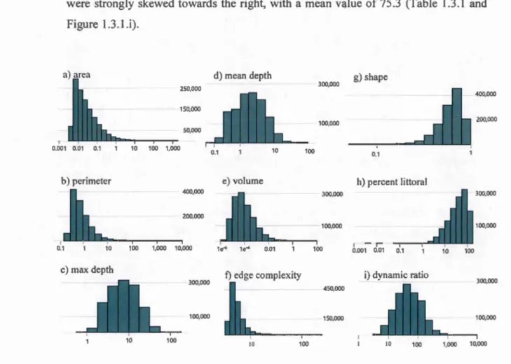
The lakes extracted covered very large ranges in ali of the morphometric parameters (Table 1.3. 1 and Figure 1.3 .1)

The shortest perimeter in the dataset is 0.25 km, whereas the longest perimeter is 5, 71 1 km and interestingly does not belong to the largest lake in the dataset. The mean perimeter length is 1.73 km, whereas the cumulative lake edge is 2,147,751 km (Table 1.3.1 ).

The empirical model based on the mean elevation change around the lake yields an average maximum depth of 9.93 m, and the range of maximum lake depths of 0.8

-144 m (Table 1.3.1). While this model may not adequately approximate depth for extreme situations such as for Lac Mistassini (max. depth 183 m) or for smaller lakes in highly variable topographies, or for kettle lakes, it was calibrated for lakes of glacier origin with surface areas between 0.005 to 1 030 km2 and 1.5 to 125 m max depth (Heath cote et al. 20 15), which represent the majority of lakes in this region and should therefore be generally suitable.

20

The calculated volumes using the above approach range severa! orders of magnitude, from 1.13·10-6 _{to 169 km}3 _{(Lac Mistassini, actual: 150 km}3

) where the mean volume is 2.6 x 1

o

-

(Table 1.3.1 ). The upper range in the distribution of mean depth (up to 143 m) is

unrealistic, however, and likely retlects bi ases in the algorithms used, but these extreme values hardly influence the overall regional lake mean depth.

The edge complexity of the lakes in Québec spans a large range, from 3.6 to 222 (Table

1.3.1 ), but with a distribution that is cl earl y skewed towards the less intricate (lower

values) part of the spectrum (Figure l.3.1.t).

The lake shape parameter approaches 0 for lakes that are perfectly round and 1 as lakes

become more oblong and elongated. The mean value and overall distribution of the

lake shape parameter, with a mean of 0.63 (Table 1.3.1 and Figure 1.3.1.g) thus

indicates that lakes in Québec tend to have more oblong shapes.

Table 1.3. 1 Summarizing statistics for Québec lakes surface areas, perimeters, depths,

volumes, edge complexities, shapes, percent littoral areas and dynamic ratios.

Lake Feature Min Max Mean Std Oev Std Err Mean Sum

urface /\rea (km') 0.005 1.369 0.15 3.14 0.003 185,762 Perimeter (km) 0.25 5.711 1.73 112 0.010 2.147.751 Maximum depth (m) 0.83 143 7 9 93 S.l4 0.007 12.295.877 Mean depth (m) 0.21 143.4 5.34 5.72 0.005 Volume (km') 1.13é 70 1 0 0026 0.15 0 0001 3.206 Edge complexity 3.57 222.4 5.65 2 74 0.002 Shape (circularity) 0.02 0.998 0.63 0.16 0.0001 Percent lilloral (%) 0.004 100 515 33.4 0.03 Dynamic ratio 4.34 7,115 76.5 94.3 0.085

1 0.001

21

That the average lake in Québec is relatively shallow is also reflected in the metric

describing the percent littoral habitat ofthese lakes. The mean percentage of the surface

area with depths that are shallower than 3 rn was 51.5%, with most' lakes ranging

between 20-80% littoral (Table 1.3.1 and Figure 1.3.1.h). Likewise, the distribution of

values of dynamic ratio, which increases as lakes go from bowl- to plate-shaped, suggest that most lakes in Québec tend to have a flat, plate-like profile, since the values were strongly skewed towards the right, with a mean v&lue of 75.3 (Table 1.3.1 and Figure 1.3.1.i).

d) mean depth g) shape

250,000 300,000 400,000 150,000 100,000 200,000 50,000 0.01 0.1 10 100 1,000 0.1 10 100 _0.1

b) perimeter e) volume h) percent littoral

400,000 _300,000 300,000 200,000 100,000 100,000 1 1 - ;-0.1 10 100 1,000 10,000 1e"' 100 0.001 0.01 c) max depth

f) edge complexity i) dynamic ratio

300,000 300,000

450,000

100,000 _150,000 100,000

10 100

10 100 10 100 1,000 10,000

Figure 1.3.1.a-i Distribution of 9 morphometric parameters for lakes with between 0.005-1,370 km2 _{surface area in Québec. Ali distributions are on a loglO}

22

1.3.2 Allometric relationships between lake metrics

We explored the relationships between the various lake metrics and lake area using

regression analysis. Ali the variables were log-transformed to ensure normality, and we further binned the variables into logarithmic-scale categories, in order to expose the

underlying patterns that are difficult to visualize due to the large density and scatter of

points.

Not surprisingly, perimeter was strongly related to lake area (R2=0.92) (Figure

1.3.2.1.a) but the log-log relationship was slightly non-linear and better captured by a

first order polynomial model.

Likewise, as lake area increases, so does the mean and maximum lake depth (R2=0.15) (Figure 1.3 .2.1.b and c), but in both cases, there was a non-linear trend where depth

tends to plateau with increasing lake size. While the range of our data is very large,

these trends offer support to the model used to estimate depth, as it in itself does not

incorporate lake size.

The mean depth tends to increase Jess with area than maximum depth and therefore the

ratio of the two tends to shi ft as lakes become larger, with consequences on the shape of the depth profile of lakes, as described below.

Volume has a strong linear log-log relationship to area (R2=0.79) (Figure 1.3.2.l.d),

which is partly attributable to surface area being a parameter in the volume algorithm.

Because depth a Iso increases with lake area, the log-slope of the relationship between

volume and area is significantly greater than 1.

The edge complexity metric also showed a wide range for any given lake area, but on average complexity tends to increase with lake size (R2=0.36) (Figure 1.3.2.l.e). This

could partially be related to the fractal nature of shorelines and the spatial resolution of

23

factor, such that a lake surface expanding over a large area in the boreal is more likely to follow a variety landscape contours than one with a smaller extent.

As mentioned before, a shape value of 1 is an almost complete diversion from a circle

and the reis a clear trend for larger lakes to converge to this value of 1 (R 2_{=0.09) (Figure}

1.3.2.1.f), suggesting that in this landscape lakes tend to become proportionally

narrower as they increase in size.

On a log-log scale, the percent of lake area overlaying sediments shallower than 3 rn

depth (% littoral) declined linearly with lake area (R2=0.17) (Figure 1.3.2.1.g).

However, this relationship was rather weak and the range in percent littoral is very

large for lakes for any given size of lake (Figure 1.3.2.l.g). Likewise, the dynamic ratio

in creas es with size (R2=0.1 0) (Figure 1.3 .2.1.h), suggesting th at although larger lakes tend to be deeper, as described above, they also tend to become more plate-like as they become larger.

We further explored the relationships that exist between the different aspects of lake

shape, and we found that there was structure in lake morphology beyond the above size

scaling (Figure 1.3.2.2). For simplicity we divided the metrics into two groups: those that depend on the depth profiles (max depth, percent littoral and dynamic ratio) and

those that are associated to shape (edge complexity and shape). The depth related

metrics ali strongly covaried, with R2 ranging from -0.75 to -0.96 and 0.70, and the two

shape metrics were also strongly coupled to each other (R2 = 0.69, Figure 1.3.2.2). The

relationships between the groups of variables were much weaker, with R2 _{ranging from}

-0.35 to -0.05 (Figure 1.3.2.2), indicating that these different dimensions of lake

morphology do not necessarily covary across the landscape, and that any given type of

- - - -- - - -- - - - -- - - -- - - -- -- - - -- -4.0 -3.0 ~ ~ ., 2.0 -E ~ 0 0, 1.0 .3 o.o 2.0 24 a) perimeter vs. area -2.0 -1.0 0.0 1.0 2.0 3.0 log10 Area (km2) Binned

c) mean depth vs. area

.

tt

.i-·2.0 ·1.0 0.0 1.0 2.0 3.0 Log10 Are• (km2) Binned

y= a) 1.01 + 0.73x + 0.04x2 b) 1.22 + 0.18x -0.02x2 c) 0.96 + 0.23x - 0.03x2 d) -1.96 + 1.28x e) 0.98 + 0.23x + 0.04x2 f) -0.12 + 0.04x -0.0 1 x2 g) 1.13 - 0.27x h) 2.06 + 0.27x + 0.02x2 x "' ~ 2.0 0 _1.0

:§'

g

d) volume vs. area

·2.0 -1.0 0.0 1.0 2.0 3.0

log10 Area (km2) Binned

RMSE R2 0.31 0.923 0.39 0.154 0.39 0.154 0.39 0.786 0.11 0.360 0.12 0.089 0.36 0.171 0.39 0.095

25

e) edge complexity vs. area f) shape vs. area

0.0 _lhill _w__ji

Log10 Area(km2) Binned Log10 Area (km2) Binned

g) percent littoral vs. area h) dynamic ratio vs. area 2.0 ... 1.0 _3.0 "ë g 0.0 :.:J 111 o'

î

Log10Area(km2) Binned Log10 Area (km2) Binn<d

Figure 1.3.2.1 Allometry regressions between ali metrics and Area. a) Perimeter (R2_=0.92),

b) Maximum Depth (R2_{=0.15), c) Mean Depth (R}2_{=0.15), d) Volume (R}2_{=0.79), e) Edge}

Complexity (R2_{=0.36), f) Shape (R}2_{=0.09), g) Percent Littoral (R}2_{=0.17), h) Dynamic Ratio}

(R2_{=0.10). The Area data have been binned, ali parameters are log-transformed and the}

whiskers of the boxes represent the quantile ranges. The fitted line through the data is

---~---

-26

~

ç======r

.

Figure 1.3.2.2 Multivariate correlation scatter-plots and correlations of the

5 metrics: Maximum Depth, Edge Complexity, Shape, Percent Littoral, and Dynamic Ratio.

1.3.3 Principal component analysis of lake metrics across the landscape We explored the distribution of sites based on the ensemble of morphometric parameters using principal components analysis (PCA), with ali input variables log-transformed to account for the large ranges and the often skewed distributions. The

resulting eigenvalues of the components quickly declined from 5.2 to 2.5 and 1.0, thus

only the first three components were retained as the most informative. These are the three dimensions of variation which is la ter used as the basis for the classification. The

*

..

-1

*

.,

\

'""

Figure 1.3.3.1 The Principal Component Analysis graphs showing the vectors of the 9 metrics across the 3 first components where the first component (57.6%) is related to size, the second one to bathymetrie shape (27.6%) and the third to Complexity (11.3%). The top plot shows

the relation between components 1 and 2, the lower plots show

components 1-3 and 2-3.

\

27

- - - -- - -

-28

PCA vectors cl earl y reflected both the importance of lake size, as weil as the allometry of lake morphology and the links that exist between specifie lake metrics.

The first axis explained up to 57.5% of the composition of the data (Figure 1.3.3.1),

and integrated severa( lake metrics, which also weighed to a lesser extent on axis 2 and

3, which explained 27.8% and 11.3% of the total variance, respectively. Mean and maximum depth, and percent littoral weighed heavily on component 1, with opposing effects which reflects that deeper lakes tend to have proportionately less shallow area and tend to be less flat. Almost orthogonally to depth Joad area, perimeter and edge complexity increase, suggesting that the larger lakes tend to have more complex shorelines but that this is relative( y independent of lake depth. Weakly increasing with the area group is the lake shape metric, suggesting that the larger lakes tend to be more oblong, however the feature is not exclusive to the large lakes.

The volume vector increases in the direction between depth and area, slightly closer to

the area, suggesting that both lake area and depth modulate lake volume. In a 90-degree angle to volume and in the same quadrant as percent littoral the dynamic ratio loads

most strongly on the 2nd component axis, again reinforcing the trend that lakes with a plate-like profile are more likely to have sediments shallower than 3 rn depth and

Figure 1.3.3.2 Bar-chart displaying the relative contribution of each metric to the 3 first PCA components. Showing more clearly that the axes can be