M. Camporese1 , C. Paniconi2 , M. Putti3, and J. J. McDonnell4
1Department of Civil, Environmental and Architectural Engineering, University of Padova, Padova, Italy,2Centre Eau Terre Environnement, Institut National de la Recherche Scientifique, Quebec, Canada,3Department of Mathematics, University of Padova, Padova, Italy,4School of Environment and Sustainability and Global Institute for Water Security, University of Saskatchewan, Saskatoon, Canada
Abstract
Integrated surface-subsurface hydrological models (ISSHMs) are well established numerical tools to investigate water flow and contaminant transport processes over a wide range of spatial and temporal scales. However, their ability to correctly reproduce the response of hydrological systems to natural and anthropogenic forcing depends largely on the accuracy of model parameterization, including the level of detail in the representation of the bedrock. This latter is typically incorporated in some way via the bottom boundary of the model domain. Issues of bedrock topography, variable soil depth, and the resulting hillslope storage distribution representation in ISSHMs are vitally important but to date have received little attention. A standard treatment of the bottom boundary, especially in large catchment and continental scale applications, is to model it as a flat or inclined (e.g., parallel to the surface) impermeable base (sometimes with some simple leakage term). This approach does not allow the model to correctly reproduce bedrock-controlled threshold responses such as the fill and spill process, as observed across many hillslope and catchment scale field studies. It is still unclear whether Richards equation-based numerical models are actually able to generate such responses. Here we use a Richards equation-based model (CATHY) to simulate internal transient subsurface stormflow dynamics observed at the well-characterized Panola experimental hillslope in Georgia (USA). Soil and bedrock properties were calibrated starting from values reported in previous studies at the site. Our simulation results show that the model was able to reproduce threshold mechanisms, which in turn affected both the integrated and distributed hydrologic responses of the Panola hillslope. We then developed a set of virtual experiments with modified boundary conditions and base topography at the soil-bedrock interface to explore the bedrock boundary control on transient groundwater flow patterns. Our results show that accurate representation of the lower boundary is crucial for ISSHM simulations of hillslope-scale storm runoff and for connectivity of transient groundwater. We summarize our findings with the development of a new bedrock topographic wetness index that takes into account the unsaturated infiltration dynamics. The index is able to help represent the spatial variability of water table response over the bedrock surface compared to standard surface topography-based indices. This new index may be useful in larger-scale ISSHM applications where an exact bedrock topography representation is not feasible or possible.1. Introduction
Recent advances in hydrogeophysics (Binley et al., 2015; Singha et al., 2015) now make it possible to charac-terize the spatial variability of bedrock topography with relatively little effort. This alleviates the information constraint on numerical models, allowing fuller investigation of the impact of a bedrock interface on hydro-logic responses and of the ability of current models to reproduce these responses (Fatichi et al., 2016). In the development of groundwater models over the past five decades, this marks a step forward analogous in some respect to, first, the transition from treating the water table as a simple specified-head bound-ary to unified models of saturated and unsaturated zone phenomena and, more recently, the advent of integrated surface-subsurface hydrological models (ISSHMs) that can resolve interactions across the land surface boundary (Paniconi & Putti, 2015).
Field and modeling experiments over a range of scales suggest that the way the bedrock interface is treated (e.g., smooth versus nonuniform, i.e., with or without microtopographic relief features, impermeable versus Key Points:
• Physics-based models reproduce the fill and spill response of hillslopes with complex bedrock geometry • Water table spatial variability can
be partly explained by a modified wetness index
• As a dominant control on groundwa-ter flow patgroundwa-terns, bedrock geometry should be accurately represented
Supporting Information: • Supporting Information S1 • Movie S1 Correspondence to: M. Camporese, [email protected] Citation: Camporese, M., Paniconi, C., Putti, M., & McDonnell, J. J. (2019). Fill and spill hillslope runoff representation with a Richards equation-based model. Water
Resources Research, 55, 8445–8462. https://doi.org/10.1029/ 2019WR025726
Received 7 JUN 2019 Accepted 24 SEP 2019
Accepted article online 15 OCT 2019 Published online 5 NOV 2019
©2019. American Geophysical Union. All Rights Reserved.
leaky, and inclusion or not of underlying formations such as fractured aquifers) has a large impact on hydro-logic response (pressure head distributions, preferential flow pathways, residence times, water table levels, groundwater recharge, groundwater-surface water interactions, streamflow discharge, etc,)( Banks et al., 2009; Buttle & McDonald, 2002; Ebel et al., 2008; Freer et al., 2002; Katsuyama et al., 2005; Kosugi et al., 2008; Uchida et al., 2002; Uchida et al., 2003). One key manifestation of bedrock-influenced processes is the fill and spill mechanism (Spence & Woo, 2003), which has been used to explain threshold-driven hillslope responses (Tromp-van Meerveld & McDonnell, 2006a).
Fill and spill is the process whereby free water forms in depressions at the soil-bedrock interface and then spills downslope over the bedrock ridge when the water level reaches the crest at the edge of a depression (Tromp-van Meerveld & McDonnell, 2006a). For fill and spill, connectivity becomes very important and contributing areas do not necessarily grow upslope from the stream channel, as conceptualized in earlier saturated wedge assumptions (Weyman, 1973). The delayed release of stored water that is characteristic of fill and spill also impacts solute transport (e.g., enhanced mixing and mass transfer in subsurface depressions) (Jackson et al., 2016), wherein the flushing frequency in the spill areas results in a stripping of weatherable products (Burns et al., 1998).
Bedrock-mediated fill and spill and associated phenomena such as threshold behaviors and connectivity-controlled flow are now well recognized experimentally; whether these processes require new theoretical frameworks and models is still an unresolved issue. New field evidence of fill and spill has led to new model approaches (Ameli et al., 2015; Janzen & McDonnell, 2015; Lehmann et al., 2007) and new theory (McDonnell et al., ??; Spence, 2010). These have been aimed largely at improving the capability of simpler approaches (e.g., low-dimensional and probabilistic models) to simulate processes associated with storage filling and connectivity spilling threshold behaviors. There has not as yet been extensive model testing of these phenomena with ISSHMs, which represent the current state of the art in hydrological modeling at the hillslope and catchment scales. Owing in part to the information constraint regarding bedrock characteristics discussed earlier, hydrological models, including ISSHMs, have traditionally relied on simplified representations of the soil-bedrock interface, generally treating it as a smooth, impermeable “surface,” sometime with a freely draining or leaky bottom boundary (e.g., Broda et al., 2011; Koussis et al., 1998; Tromp-van Meerveld & Weiler, 2008). Other studies have set the bottom boundary of the model domain deeper than the soil-bedrock interface (Ebel et al., 2007, 2008).
A small handful of physics-based modeling studies have taken into account detailed representation of bedrock features (Ameli et al., 2015; Hopp & McDonnell, 2009; James et al., 2010; Lanni et al., 2013). These studies have all been done at the Panola Mountain Research Watershed, an experimental trenched hills-lope in Georgia (USA) with a comprehensive observational data set of hydrologic and hydrostratigraphic variables. The present study builds on this previous work and investigates whether physics-based models, fed with accurate and representative data, can properly simulate the behavior of complex hydrological sys-tems and provide useful insights into the development of threshold-driven responses. We use the CATHY (CATchment HYdrology) simulator (Camporese et al., 2010; Weill et al., 2011), an ISSHM that uses rigorous numerics to solve the mass conservation equations governing water flow and solute transport. ISSHMs are well tested (Kollet et al., 2017; Maxwell et al., 2014) and increasingly used in diverse applications, including at continental scales (e.g., Condon & Maxwell, 2015; Lemieux et al., 2008), where open questions remain regarding the representation and role of bedrock boundaries and formations. Our objective is to run the model with different soil depths, bedrock depths, bedrock resolutions, and boundary conditions, in order to explore the level of accuracy required to capture the threshold-driven response of systems like the Panola hillslope and to assess the capability of various topographic wetness indices to explain the spatial variability of observed water table responses and connectivity at the soil-bedrock interface, including a new index that accounts for unsaturated zone dynamics.
2. Methods
2.1. Study Area
The study site is the Panola experimental trenched hillslope, a forested hillslope located within the Panola Mountain State Conservation Park, in the state of Georgia (USA). The climate at the Panola Mountain State Conservation Park is humid continental to subtropical, with average temperature and annual precipitation of 15.2◦C and 1,220 mm, respectively (NOAA, 1991; Peters et al., 2003). Winter rainfall events are typically
Figure 1. (a) Three-dimensional finite element mesh of the Panola hillslope. (b) Map of the soil-bedrock interface elevation. (c) Map of the soil thickness. The color bars indicate elevation (m) in (a) and (b) and thickness (m) in (c).
long, low-intensity rainstorms, while short and intense convective thunderstorms are common in spring and summer.
Over the last 25 years, experimental investigations on the Panola hillslope have contributed important knowledge about threshold rainfall-runoff response and its relation to patterns of transient water table development. A comprehensive set of climate, hydrogeological, and hydrological data are publicly available (Tromp-van Meerveld et al., 2008), which provide a full description of the assembled data types, their orga-nization, and their origins. In this study, we used the 2002 rainfall-runoff data set as it includes extensive spatiotemporal measurements of internal hillslope hydrological response, in the form of water table devel-opment, and subsurface stormflow delivered to a trench that was specifically excavated for rainfall-runoff data collection. The trench extends vertically to the interface between the soil and the bedrock. For more detailed information on the Panola hillslope and data collection, see the http://www.sfu.ca/PanolaData/ index.htm website. Hereafter, water table is relative to the soil-bedrock interface, unless otherwise specified.
2.2. Numerical Model
The CATHY (CATchment HYdrology) numerical model (Camporese et al., 2010) is one of several ISSHMs recently developed with an overall goal of providing a holistic representation of hydrological processes in different compartments of terrestrial systems at scales ranging from hillslope to continental.
CATHY consists of a finite element solver of the three-dimensional Richards equation for water flow in partially saturated porous media coupled with a path-based finite difference solution of the zero-inertia wave approximation of the Saint-Venant equation for surface water dynamics. Coupling between the two computational domains is obtained through a time-splitting and boundary condition-switching procedure that ensures continuity at the surface-subsurface interface (Camporese et al., 2010, 2014). Other features implemented in the model include solute transport (Weill et al., 2011) and data assimilation (Camporese et al., 2009).
2.3. Model Setup and Calibration
As in James et al. (2010), the model grid (Figure 1) was built to accurately represent the geology of the Panola hillslope, consisting of a layer of sandy loam overlying a weathered granite bedrock. The soil thickness is variable in space, ranging from 0.12 to 1.86 m, based on field estimations with soil corer and hand auger, while the bedrock is represented, in this present study, with a 1-m uniform thickness. The soil zone is dis-cretized into 16 computational layers of variable thickness and the bedrock formation into four layers of uniform (25 cm) thickness. Combined with a surface digital terrain model of 1-m resolution, this results in a finite element mesh of 23,100 nodes and 123,480 elements.
Boundary conditions for all simulations were assigned as follows: water fluxes corresponding to throughfall estimated from rainfall data at the surface boundary (evapotranspiration was considered negligible as the simulated periods correspond to the winter season)( James et al., 2010; Keim et al., 2006); no flow across the lateral boundaries, except for the downslope one, where a seepage face (limited to the soil numerical layers)
Table 1
Soil and Bedrock Parameter Values Used in This Study Compared to the Corresponding Values in James et al. (2010) Material type Ks(m/s) Ss(m−1) 𝜙(—) 𝛼(cm−1) n(—) 𝜃 r(—) Present study Soil 2.6×10⁻³ a 5.0×10⁻³ 0.58 0.362a 1.26a 0.09 Bedrock 2.1×10⁻⁶a 5.0×10⁻³ 0.33 0.305a 1.26a 0.09 James et al. (2010) Soil 2.5×10⁻⁴ N/A 0.58 0.706 1.25 0.09 Bedrock 2.5×10⁻⁶ N/A 0.33 0.196 1.25 0.09
Note. N/A = not applicable.aCalibrated.
was used to reproduce trenchflow; and free drainage across the bottom boundary (base of the 1-m bedrock layer) to reproduce deep percolation. Two precipitation events were simulated. The first event occurred on 8 February 2002 and consisted of a 24-hr low-intensity rainstorm. The second event occurred on 30 March 2002 and consisted of a short, high-intensity convective thunderstorm. It was only during these two largest rainstorms of 2002 that an extensive saturation at the soil-bedrock interface occurred, which led to a signifi-cant hillslope response in terms of trenchflow (Tromp-van Meerveld et al., 2008). Here we focus our attention on the 30 March 2002 thunderstorm, which was used for parameter calibration and testing of different sce-narios, while the 8 February 2002 rainstorm was used for validation purposes only. In both cases, model initialization was achieved by running a long warm-up simulation with measured atmospheric forcing, to achieve realistic initial conditions at the beginning of the event under consideration. Warm-up periods were from 9 February 2002 and from 1 January 2002, for calibration and validation, respectively, meaning that the two simulation periods never overlap each other.
Parameter calibration was carried out by means of the shuffled complex evolution method (Duan et al., 1994). The objective of the calibration was to find a set of soil and bedrock parameters that minimizes the root-mean-square error between observed and simulated trenchflow for the 30 March 2002 thunderstorm. Observed trenchflow is defined here as the total of matrix and macropore flow (Tromp-van Meerveld & McDonnell, 2006a). We opted to not include other data types in the objective function in order to avoid a complex multiobjective calibration exercise and because we wished to assess whether a model parameteri-zation optimizing the hillslope integrated response resulted in (1) a realistic representation of the transient water table patterning and (2) a correct representation of the emergent fill and spill behavior driving the trenchflow. The calibrated parameters were the saturated hydraulic conductivity, Ks, and the shape param-eters,𝛼 and n, of the soil hydraulic functions (van Genuchten, 1980). All other soil and bedrock parameters (specific storage coefficient, Ss, porosity,𝜙, and residual water content, 𝜃r) were either taken from James et al. (2010) (𝛷 and 𝜃r) or assigned based on experience (Ss).
Table 1 reports the soil and bedrock parameters resulting from the calibration as well as the fixed parameters. Even though anisotropy was allowed in the calibration procedure for the hydraulic conductivity, the shuffled complex evolution algorithm converged to isotropic Ksvalues. The final values of the calibrated parameters are close to the values suggested by James et al. (2010), except for the sandy loam soil, for which we found a value of Ksthat is an order of magnitude larger.
2.4. Synthetic Experiments
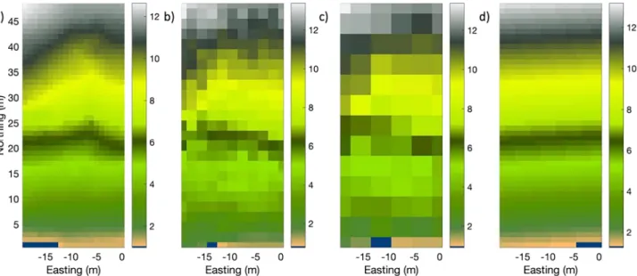
Following model calibration, henceforth referred to as the reference simulation, we conducted a number of synthetic experiments (summarized in Table 2) to explore the influence on the hillslope water budget and flow patterns of (i) the thickness of the bedrock formation, (ii) the boundary conditions at the bottom of the bedrock (free drainage vs. no flow), (iii) the soil thickness (spatially variable versus uniform), and (iv) the geometry of the soil-bedrock interface. In this last factor we included two common assumptions used in ISSHM modeling, typically as a result of lack of data: a soil-bedrock interface that is parallel to the surface and a soil-bedrock interface represented by a straight sloping plane. Four of the soil-bedrock configurations used are shown in Figure 2. All the scenarios described in Table 2 were carried out using the same 30 March 2002 rainfall event as in the reference simulation and with the same warm-up procedure to generate the initial conditions.
Table 2
Summary Description of the Reference Simulation and Synthetic Experiments
Scenario tag Bedrock thickness Bottom boundary conditions Soil thickness Soil-bedrock interface Reference 1 m Free drainage Spatially variable, from Spatially variable, from
measured data measured data
Deep10_fd 10 m NC NC NC
Deep10_nf 10 m No flow NC NC
Deep50_fd 50 m NC NC NC
Deep50_nf 50 m No flow NC NC
Parallel_1 NC NC Uniform (1 m) Soil surface parallel
to measured soil-bedrock interface
Parallel_2 NC NC Uniform (1 m) Soil-bedrock interface parallel to
Reference (measured) soil surface
Coarse_2 NC NC NC Reference soil-bedrock interface
but coarsened to 2 m resolution
Coarse_4 NC NC NC Reference soil-bedrock interface
but coarsened to 4 m resolution
Straight NC NC NC Soil-bedrock interface
is a straight sloping plane Note.NC = not changed with respect to the Reference simulation.
2.5. Topographic Wetness Indices
In addition to the simulation experiments described above, we also investigated the capability of various topographic wetness indices to explain the spatial variability of the distributed response and the connectivity patterns over the soil-bedrock interface in the Panola hillslope. Along with the standard topographic wetness index of the surface topography, TWI (Beven & Kirkby, 1979),
TWI =ln(a∕ tan𝛽), (1)
where a is the upslope contributing area per unit contour length and tan𝛽 is the local slope, we considered here also its equivalent for the bedrock topography, TWIbr, where a and tan𝛽 are now computed from the geometry of the soil-bedrock interface. As neither TWI nor TWIbrtake into account the soil hydraulic prop-erties, we also examined two variants that include soil thickness, D, time-averaged infiltration rate, I, and
Figure 2. Map of the soil-bedrock interface for four of the scenarios reported in Table 2: (a) Parallel_2, (b) Coarse_2, (c) Coarse_4, and (d) Straight. All other scenarios have the same soil-bedrock interface as the reference simulation (see Figure 1).
saturated or unsaturated hydraulic conductivity: STW Isat=ln Ia KsDtan𝛽 , (2) STW Iuns=ln Ia K(𝜓D)Dtan𝛽 , (3)
where K(𝜓D)is computed with the calibrated van Genuchten curve assuming pressure head,𝜓, equal to negative soil thickness, −D. Note that STWIsatand STWIunsare dimensionless and that the products KsD
and K(𝜓D)Dare indicators of soil transmissivity, wherein the former assumes a fully saturated soil while the latter takes into account the spatially varying saturation state. As for TWIbr, a and tan𝛽 are calculated from the soil-bedrock interface also for STWIsatand STWIuns.
The performance of the wetness indices was evaluated first by computing their Pearson and Spearman rank correlation coefficients with the water table spatial distribution at the moment of maximum storage during the simulation. To further expand this analysis, following Lanni et al. (2011), we investigated the capability of the wetness indices to explain the subsurface connectivity paths. To this aim, the maps of pressure head over the soil-bedrock interface and wetness index were converted into binary maps (wet/dry) defined by an indicator function I(zi;zk), equal to 1 (wet) if zi ≥ zkand 0 (dry) otherwise, where ziis the value of the wetness index or pressure head in node i and zkis a chosen threshold value separating dry from wet areas. Another indicator function I(zi;zk), equal to 0 if zi ≥ zkand 1 otherwise, was used to ensure that ∑N
i=1I(zi;zk)I(zi;zk) =N, N being the number of surface nodes in the finite element mesh. The following similarity coefficients were computed:
𝜆 = ∑N i=1I(W Ii;W Ik)I(𝜓i;𝜓k) ∑N i=1I(W Ii;W Ik)I(𝜓i;𝜓k) + ∑N i=1I(W Ii;W Ik)I(𝜓i;𝜓k) , (4) 𝜇 = ∑N i=1I(W Ii;W Ik)I(𝜓i;𝜓k) ∑N i=1I(W Ii;W Ik)I(𝜓i;𝜓k) + ∑N i=1I(W Ii;W Ik)I(𝜓i;𝜓k) , (5) SM = ∑N i=1I(W Ii;W Ik)I(𝜓i;𝜓k) + ∑N i=1I(W Ii;W Ik)I(𝜓i;𝜓k) N , (6) SC = ∑N i=1I(W Ii;W Ik)I(𝜓i;𝜓k) ∑N i=1I(𝜓i;𝜓k) , (7) Ck= SM − RA 1 − RA , (8)
where WI represents the wetness index being considered (TWI, TWIbr, STWIsat, or STWIuns). The coefficients
𝜆 and 𝜇 indicate the rates of false negatives and false positives, respectively, while SM is a measure of simple
matching, SC of direct spatial coincidence, and Ckis the Cohen's kappa coefficient (Lanni et al., 2011), which takes into account the overall probability of random agreement, RA:
RA = ∑N i=1I(W Ii;W Ik) N ∑N i=1I(𝜓i;𝜓k) N + ∑N i=1I(W Ii;W Ik) N ∑N i=1I(𝜓i;𝜓k) N . (9)
To produce time-independent connectivity patterns over the soil-bedrock interface, we conducted steady-state simulations assuming a constant throughfall of 1.0×10⁻⁶m/s (3.6 mm/hr). This led to constant distributions of pressure head over the soil-bedrock interface. Two pressure head thresholds were tested to distinguish dry from wet soil areas:𝜓 = 0.0 m and 𝜓 = −8.87 × 10⁻⁴m, the former being the conventional definition of a water table and the latter being the air entry pressure head corresponding to the calibrated van Genuchten retention curve (Or et al., 2015), thus accounting for possible effects of the capillary fringe. For each wetness index, 19 possible thresholds were considered, corresponding to percentiles ranging from the 5th to the 95th with a step of five.
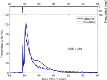
Figure 3. Observed and modeled trenchflow for the 30 March 2002 thunderstorm simulation. NSE is Nash-Sutcliffe efficiency.
3. Results
3.1. Reference Simulation: Measured Bedrock Geometry With Calibrated Parameters
Figure 3 shows the comparison between observed and modeled trenchflow for the 30 March 2002 simula-tion. The agreement is quite good, with a Nash-Sutcliffe coefficient of 0.86, even though the model exhibits a slightly faster recession phase compared to the observed one. This is probably due to the choice of the objective function in the calibration algorithm (root-mean-square error), which tends to give more weight to the peaks rather than the recession phases. The total volume of the hydrograph is also well captured by the model. Figure 4 compares simulated and observed trenchflow for the 8 February 2002 validation event. The model performance is not as good as for the calibration event, but it is nonetheless satisfac-tory (Nash-Sutcliffe coefficient of 0.72), providing confidence that the model is realistically reproducing the hydrological dynamics in the hillslope.
We now analyze in detail the results of the 30 March 2002 simulation in terms of the internal distributed response of the hillslope. Two types of water table data are available in the Panola hillslope: maximum water level rise at the soil-bedrock interface, measured with 135 crest-stage gauges, and continuous water level, measured in a series of 29 water table recording wells located along two downslope transects and within a bedrock hollow (Tromp-van Meerveld & McDonnell, 2006a).
Figure 4. Observed and modeled trenchflow for the 8 February 2002 rainstorm simulation. NSE is Nash-Sutcliffe efficiency.
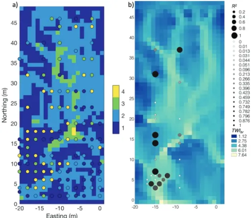
Figure 5. (a) Simulated maximum water level rise above the soil-bedrock interface in response to the 30 March 2002 rainstorm. The circles represent corresponding measurements from the crest-stage gauges (James et al., 2010). Both simulated and measured values are binned in the categories of 4 = high (>20 cm), 3 = medium (10–20 cm), 2 = low (<10 cm), and 1 = no (0 cm) rise. (b) Squared correlation coefficient (equivalent to coefficient of determination, R2) of simulated versus observed water table in 29 continuously monitored boreholes for the 30 March 2002 rainstorm. The color bar corresponds to the topographic wetness index of the soil-bedrock interface, while both size and color of the circles vary as a function of the R2values.
Figure 5a shows the maximum water level rise over the soil-bedrock interface modeled in the 30 March 2002 simulation, compared with the crest-stage measurements. The reported values are binned in categories of high (>20 cm), medium (10–20 cm), low (<10 cm), and no (0 cm) rise. The maximum values simulated by CATHY generally fall below those observed (e.g., highest modeled maxima of about 30 cm against mea-sured values of more than 40 cm), probably due to the fact that parameter calibration was carried out against trenchflow data only. However, the spatial patterns are in broad qualitative agreement. Comparing simply whether the water table at the soil-bedrock interface responds or not, out of 116 available observations, the model and measurements agree in 89 locations, while in 16 cases the model simulates a response that was not observed and in other 11 cases the model fails to show an observed response (see also Figure S1 in the supporting information). There is also a clear correlation between the simulated maximum water table rise in Figure 5a and the topographic wetness index of the soil-bedrock interface, TWIbr(Figure 5b). This is in agreement with previous results for the Panola hillslope (Freer et al., 2002). Figure 5b also shows the squared correlation coefficient, R2, between measured and simulated water level (the latter extracted at the position of each of the 29 recording wells) calculated over the entire simulation. Once again, despite a general under-estimation of the water table data by the model, the subsurface dynamics is captured fairly well, especially along the main subsurface flow paths identified by high values of TWIbr. Points with R2 = 1(large black circles) indicate boreholes where neither the model nor the measurements detected any response. Overall, there is qualitative agreement between model and observations for 21 of the 29 recording wells. In four other cases the model simulates a response while the observations do not show any response, and in the remaining four cases the opposite occurs.
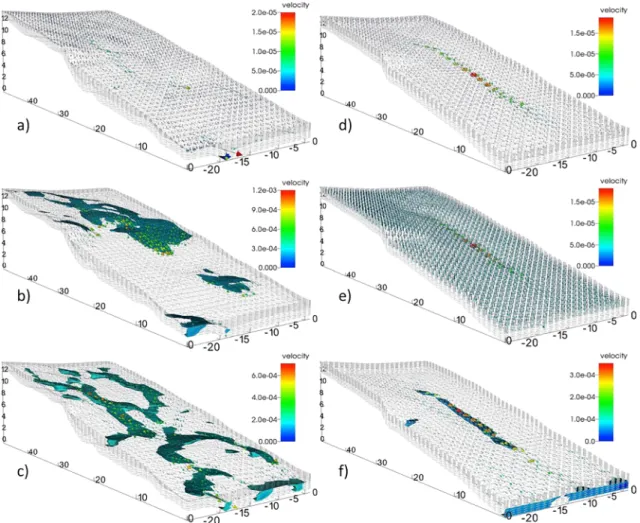
Figure 6. Snapshots of simulated Darcy velocity and extent of water buildup (shown by isovolumes bounded by pressure head values between 0 and 0.3 m) over the soil-bedrock interface for (a–c) the Reference scenario and (d–f) the Parallel_2 scenario, at times (a and d) 88.3 day, (b and e) 88.9 day, and (c and f) 89.1 day. Distances are in meters and velocities in meters per second.
In Figures 6a–6c, as well as in the movie provided in the supporting information that shows the modeled subsurface response over the duration of the simulation, it can be seen how the hillslope, initially unsatu-rated, is first subject to vertical infiltration (panel a), followed by the development of a complex pattern of perched water table (panels b and c) that results from the progressive filling and connecting of upslope and downslope depressions in the soil-bedrock interface. As a consequence, Darcy fluxes are concentrated in the flow paths connecting these depressions, with maximum computed flow velocities of about 10−3m/s. This is consistent with estimates by Tromp-van Meerveld and McDonnell (2006b), who obtained, based on various measurements, flux velocities of 8 m/hr (2.2 × 10⁻³m/s). The video clearly shows that the main contribu-tion to the trenchflow comes from the left-hand side porcontribu-tion of the hillslope, in agreement with previous experimental analyses (Tromp-van Meerveld & McDonnell, 2006a).
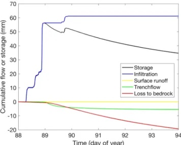
We also analyze, in Figure 7, the different terms of the water balance in the hillslope for the 30 March 2002 rainstorm simulation, including the cumulative input (infiltration) and output (surface runoff, trenchflow, and loss to bedrock) fluxes, together with the time evolution of total subsurface storage. Surface runoff out-flow is always negligible, consistent with observations (Tromp-van Meerveld & McDonnell, 2006b), although the CATHY surface module was very briefly activated at the beginning of the rainstorm, resulting in a small amount of Hortonian overland flow that reinfiltrated downslope. This also agrees with previous literature: James et al. (2010) reported, for high-intensity storms, indirect evidence of overland flow (such as displaced leaves), on small portions of the hillslope below bedrock outcrops that quickly reinfiltrated. The final val-ues of trenchflow, loss to bedrock, and storage change account for about 10%, 30%, and 60% of infiltration, respectively. By comparison, James et al. (2010) reported estimates based on measurements of 11%, 71%, and 18%, respectively. We note that our simulation yields a comparable percentage of trenchflow, whereas the
Figure 7. Time evolution of different terms of the water balance during the simulation of the 30 March 2002 rainstorm.
disagreement with the estimates of storage change and loss to bedrock can probably be explained by a differ-ent domain of integration for the bedrock layers. If we compare instead to the modeled estimates reported in James et al. (2010), simulated with TOUGH2, our computed water budget terms are in closer agreement, notwithstanding a difference in the soil to bedrock Ksratio (1000:1 for CATHY and 5000:1 in James et al. (2010)).
3.2. Synthetic Experiments: Modified Bedrock and Soil Geometries
Having thus demonstrated an adequate correspondence between simulations and observations for the Panola hillslope, in terms of both hydrograph and water table response, we will further explore, in this section, bedrock-driven thresholding behavior with the numerical model for the scenarios reported in Table 2.
Table 3 summarizes the percent differences in the water balance terms of the virtual scenarios relative to the reference simulation. It is immediately apparent that the boundary conditions at the bottom of the bedrock layer (no flow versus free drainage) have a paramount influence on the hillslope response, the no flow scenar-ios showing dramatic changes with respect to the reference simulation. With the same boundary conditions (free drainage), the scenario with the 10-m-deep bedrock is quite similar to the reference run, while the 50-m-deep case, being affected by a much larger initial storage, exhibits an overestimated loss to bedrock and, as a consequence, a largely negative storage change and underestimated trenchflow.
The two parallel scenarios give important indications on the relative roles of soil thickness and soil-bedrock interface on the hillslope response. Both runs are characterized by a uniform soil thickness of 1 m, but the
Table 3
Changes in Water Balance for the Simulations With the Modified Bedrock and Soil Geometries and the Modified Bottom Boundary Conditions Compared to the Reference Simulation Scenario tag 𝛥trenchflow (%) 𝛥storage change (%) 𝛥loss to bedrock (%)
Deep10_fd +7 +8 −11 Deep10_nf +710 −57 −100 Deep50_fd −66 −239 +477 Deep50_nf +1,150 −118 −100 Parallel_1 +7 +2 +6 Parallel_2 −12 +23 −40 Coarse_2 +10 −20 +38 Coarse_4 −5 −16 +87 Straight −17 +31 −43
Figure 8. Simulated trenchflow for the reference and synthetic scenarios described in Table 2 for the 30 March 2002 rainstorm.
first one has the same soil-bedrock interface as the reference simulation and produces less deviation in the water balance terms. The second scenario has a (virtual) soil-bedrock interface parallel to the (measured) surface and produces much larger differences. This is evidence that at Panola the hillslope response is mainly controlled by the soil-bedrock interface geometry, with soil thickness exercising a second-order control. The last three scenarios in Table 3 feature a progressive coarsening of the soil-bedrock interface resolution. In Coarse_2, a 2-m resolution was used instead of the original 1-m resolution, resulting in appreciable changes of the water balance terms but still smaller than other scenarios such as Deep50_fd or Parallel_2. With a 4-m resolution, there is a large increase in the loss to bedrock, associated with an underestimation of the trenchflow. Finally, using a straight sloping plane for the soil-bedrock interface results in the largest differences, especially in terms of trenchflow underestimation.
Figure 8, which shows the simulated trenchflow for the virtual scenarios, and Figure 9, which reports the corresponding maximum water table rise over the soil-bedrock interface, confirm the inferences drawn from Table 3. The simulations with deeper bedrock and no flow boundary conditions resulted in sustained base-flow caused by return base-flow from the bedrock, as is apparent from Figure 9e, which exhibits an area of water accumulation immediately upstream of the trench. A bedrock depth of 50 m with free drainage bound-ary conditions yielded almost no trenchflow and water table response, while the Deep10_fd run simulated a response very similar to the reference run. Similar to Deep50_nf, the Deep10_nf run exhibits a slightly larger extent of saturation upstream of the trench compared to Deep10_fd, which is sufficient to explain the larger baseflow. Of the two parallel scenarios, the one with a “wrong” soil-bedrock interface resulted in a largely dampened trenchflow hydrograph and limited water table response relative to the reference, while the one with measured bedrock geometry but uniform soil thickness had a qualitatively similar trenchflow dynamics, albeit generally overestimated, and a similar water table rise distribution. Figure 9h and the bot-tom panel of Figure 8 demonstrate how coarsening the resolution of the soil-bedrock interface from 1 to 2 m did not result in dramatic changes of trenchflow and water table rise, although a slight overestimation of the main peak of the hydrograph did occur. A further coarsening to 4 m led to significant inaccuracies in
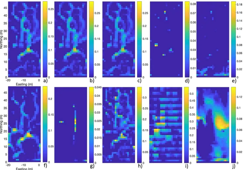
Figure 9. Simulated maximum water table rise over the soil-bedrock interface for scenarios (see also Table 2): (a) Reference, (b) Deep10_fd, (c) Deep10_nf, (d) Deep50_fd, (e) Deep50_nf, (f) Parallel_1, (g) Parallel_2, (h) Coarse_2, (i) Coarse_4, (j) Straight. Note that the color scales are not the same for all the panels.
the description of both trenchflow (Figure 8) and water table response (Figure 9i), while a straight bedrock geometry (Figure 9j) not surprisingly completely altered the response of the hillslope.
3.3. Performance of Topographic Wetness Indices
From a visual inspection of the water table results for the reference run (Figure 6), it would seem that the TWI of the soil-bedrock interface is a good indicator of subsurface dynamics, as reported also by Freer et al. (2002). We examined this relationship for the 30 March 2002 rainstorm by computing the correlation between the water table rise over bedrock at the time of peak subsurface storage and the topographic wetness indices presented in section 2.5.
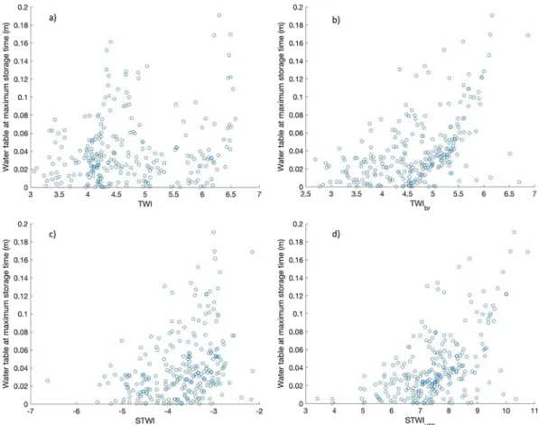
Figure 10 shows the relationships between the four topographic indices and the water table at the time of peak subsurface storage for the reference simulation, while Table 4 summarizes the correlation values, expressed in terms of both Pearson and Spearman rank correlation coefficients, the latter accounting for possible effects of nonlinearity. It is clear that the standard TWI is a poor indicator of water table spatial variability, while TWIbris much better at explaining the water table dynamics. Interestingly, STWIsatis sig-nificantly worse than TWIbr, whereas STWIuns, thanks to the additional spatial variability taken into account with the unsaturated hydraulic conductivity, yields appreciably larger correlations.
Figure 11 reports the similarity coefficients of equations (4)–(8) for the indices TWIbr, STWIsat, and STWIuns, as a function of wetness index thresholds and the two definitions of wet versus dry areas, as described in section 2.5. The patterns are very similar for all the wetness indices. However, it is clear that, with a fixed
Figure 10. Scatter plots of simulated water table level at peak subsurface storage and different topographic wetness indices for the reference simulation: (a) TWI of surface topography, (b) TWIbrof soil-bedrock interface, (c) STWIsat (equation (2)), and (d) STWIuns(equation (3)). TWI = Topographic Wetness Index.
definition of wet/dry areas (either𝜓 = 0.0 or −8.87 × 10⁻⁴m), the proposed index STWI
uns outperforms TWIbrand STWIsatfor a broad range of percentiles (from 20 to 75), as evidenced by a smaller count of false negatives (𝜆) and positives (𝜇) and larger simple matching (SM), spatial coincidence (SC), and Cohen's kappa (Ck) similarity coefficient values. This is particularly apparent for Ckand𝜆 in the range of percentiles from 50 to 75.
4. Discussion
4.1. Ability of Richards Equation-Based Models to Represent Hillslope Fill and Spill
The physically based ISSHM CATHY was set up and calibrated to reproduce the integrated and distributed response of the Panola hillslope, characterized by a complex bedrock topography. The simulations using the measured bedrock topography demonstrated that a Richards equation-based model, without additional parameterization or other enhancements, is able to capture the main features of the threshold-driven, fill, and spill-type hydrological response observed at Panola, reproducing satisfactorily both the trench-flow and water table rise measurements. This result shows that an ISSHM is indeed able to reproduce
Table 4
Correlation Coefficients Between Simulated Water Table at Peak Subsurface Storage for the Reference Simulation and Various Topographic Wetness Indices
Index Pearson Spearman
TWI 0.1889 0.1399
TWIbr 0.5084 0.5084
STWIsat 0.3472 0.3751
Figure 11. Similarity coefficients of the proposed topographic wetness indices with varying percentile thresholds and two different definitions of wet versus dry areas above the soil-bedrock interface. TWI = Topographic Wetness Index.
bedrock-controlled fill and spill processes. This contrasts with James et al. (2010), who were unable to find a parameterization for the TOUGH2 model that could satisfactorily reproduce both trenchflow and water table response for the 30 March 2002 Panola rainstorm. This was likely due to their simplification of the bedrock model layers, allowing for dynamics along the vertical direction but not the lateral directions. Good model performances have been achieved in other numerical studies of the Panola hillslope (Hopp & McDon-nell, 2009; Ameli et al., 2015) using the Hydrus-3D and HydroGeoSphere models, respectively. In both these studies, however, model verification was focused on trenchflow and matric potential in the unsaturated zone and not on the distributed water table response over the soil-bedrock interface. It should be noted that the hydraulic conductivities found in this present work are broadly consistent with those reported in previous Panola modeling studies, especially the bedrock values. However, Ameli et al. (2015) obtained a Ksvalue of the soil layer of about 640 mm/hr, whereas our value (9,360 mm/hr) is closer to the one reported by Hopp & McDonnell (2009; 3,500 mm/hr), which was not calibrated but assumed based on field observations. It is also worth noting that both Hopp and McDonnell (2009) and Ameli et al. (2015) used a transition layer between the soil and the underlying granite, in contrast to the simple two-layer configuration used here. It is of course difficult to make precise comparisons between our results and previous studies, owing to the complexity of the Panola hillslope system and the model forcings used. The inverse problem at the core of the model calibration phase is typically ill posed, with possibly multiple parameterizations leading to similar responses. Additionally, the inherent scarcity of measurements in relation to the complexity of the processes allows only an incomplete characterization of the system. Our results show that a systematic use of bedrock geometry data resulted in predicted states of reasonable accuracy without the need to introduce additional processes into CATHY. Although it has been reported that lateral pipe flow plays an important role in sub-surface stormflow at the Panola hillslope (Tromp-van Meerveld & McDonnell, 2006b; Uchida et al., 2005), not enough information regarding the geometry and distribution of the soil pipes is available upon which to base alternative approaches, for example, dual continuum. The relatively high value for Ksfound by CATHY may indeed reflect indirectly the preferential flow impacts on lateral downslope flow at the soil-bedrock interface as reported elsewhere (Graham et al., 2010). Nevertheless, the use of a dual continuum approach to simulate pipe flow at the Panola hillslope would necessarily increase the parameter set, ultimately leading to even larger uncertainties in the results due to increased ill posedness.
A series of synthetic experiments with modified boundary conditions, soil thickness, and representations of the bedrock topography illustrated a number of issues associated with the common assumptions in ISSHM applications at the hillslope scale (e.g., assumptions of smooth and linear soil-bedrock interfaces or deep bedrock formations with no flow boundary conditions). No previous study of the Panola hillslope has addressed these issues. Our results showed that such assumptions can lead to large errors. Our results also showed that relatively small uncertainties in the definition of the soil-bedrock interface can result in sig-nificant differences in the various terms of the water balance. For instance, we found that a deep bedrock formation with no flow boundary conditions at the base does not always ensure a correct representation of the flow and water table patterns. Moreover, for the configuration with “real” surface topography but with the soil-bedrock interface assumed parallel to the surface, it was impossible to capture the Panola hillslope's fill and spill dynamics, leading to a delayed and damped hydrological response. In contrast, we also showed that the configuration with measured bedrock geometry but uniform soil thickness yielded results that were closer to the reference simulation. This suggests that the soil-bedrock interface geometry can exercise a more important control on hillslope response than soil thickness. This follows other studies (e.g., Bertoldi et al., 2006) that found that soil thickness alone had a weaker control on the various terms of the catchment water budget compared to other geomorphic variables such as terrain slope and the river network length. Other important implications of our study derive from the observation that a progressive coarsening of the soil-bedrock interface resolution (from 1 m to a representation of the interface as a straight surface with an average slope) rapidly leads to a model incapable of reproducing the real hillslope dynamics and water budget terms. Whether this has significant consequences on Earth system modeling at continental or global scales, where typically the resolution does not allow a detailed description of the bedrock geometry, warrants future investigations (and is discussed in section 4.3).
4.2. On the Usefulness of Index Approaches
The Earth system modeling community also recognizes the important role played by the bedrock in con-trolling hydrological fluxes in hillslopes and catchments (e.g., Fan et al., 2019). However, how to upscale processes to the typical resolution of Earth system models, that is, ∼20–200 km, remains a formidable chal-lenge. A possible step forward in this direction can perhaps stem from the development and application of wetness indices for the bedrock geometry, similar to the well-known TWI (Beven & Kirkby, 1979), originally proposed to predict the location of saturated areas from readily available topographic data. Of course, this index has subsequently been used in many other variants and for various purposes, for example, to identify sources of subsurface flow; to estimate the hydrological, physical, and chemical properties of soils; to charac-terize vegetation patterns; or to investigate scaling effects (Ali et al., 2014). Freer et al. (2002) already showed that the bedrock-derived upslope accumulated area can be a good predictor of the water table response in the Panola hillslope, ultimately controlling the subsurface storm flow response. This suggests that variants of the TWI that include soil information, such as soil depth and hydraulic conductivity, that is, soil topo-graphic wetness indices (STWIs), if derived from the bedrock geometry, may have the capability to describe the saturated connectivity patterns forming at the soil-bedrock interface which are then responsible for threshold-driven hydrological responses.
Within this context, we conducted further analyses of the simulation results to explore the potential of var-ious topography- and bedrock-derived wetness indices to be used as predictors of saturated connectivity patterns within the hillslope. These analyses show that the standard TWI, as expected, could not explain the spatial variability of the water table. On the other hand, an analogous index derived from the bedrock rather than land surface topography resulted in good correlations with the saturation distribution over the soil-bedrock interface. This can be further improved by taking into account the soil thickness and unsat-urated hydraulic conductivity. The newly proposed index, STWIuns, represents a potentially useful tool to visualize the tendency of catchments or hillslopes to produce threshold-driven hydrological responses. However, it is worth noting that, although statistically significant, none of the correlation and similarity coefficients exceeds 0.6, indicating that no topographic index (yet) can capture the full complexity of water table dynamics as can be done in physics-based models.
4.3. Beyond the Hillslope Scale
Overall, our results corroborate the fact that, if a sufficiently accurate geometrical characterization of the active boundary of the process domain is available, the calibration of a horizontally homogeneous parame-terization leads to reasonably accurate and robust ISSHM predictions. This is consistent with the dissipative character of Richards equation and the existence of a maximum principle (Celia et al., 1990), whereby
boundary conditions dictate the solution in the domain interior. This conclusion can have important impli-cations also for larger-scale appliimpli-cations of ISSHMs, where the simplified parallel-to-surface paradigm is often used (e.g., Condon & Maxwell, 2015; Lemieux et al., 2008).
Scaling issues are pervasive in hydrological science and have been studied extensively in the literature (Blöschl & Sivapalan, 1995; Beven, 2002; Hrachowitz & Clark, 2017); nevertheless, upscaling frameworks remain elusive. We argue that the collection of extensive subsurface structural data, beyond the drilling of a few boreholes, should be an important part of hillslope and catchment characterization. Rapid advances and improvements in hydrogeophysical methods (Binley et al., 2015) such as direct current resistivity, ground penetrating radar, and electromagnetic surveys (including airborne)( e.g., Vittecoq et al., 2019) pro-vide unprecedented opportunities to improve the field characterization of groundwater storage mechanisms in catchments (e.g., Cochand et al., 2019; Staudinger et al., 2017) and to build the multiscale data sets (e.g., Pelletier et al., 2016; Shangguan et al., 2017; Xu & Liu, 2017) needed to develop mathematically and physically sound methodologies (e.g., Heimsath et al., 1997; Nicótina et al., 2011; Pelletier, 2013) for upscaling local observations, such as bedrock information from borehole data.
Lastly, parameterizing at the macroscale, the effects of relatively microscale processes at the hillslope are indeed a grand challenge. The large catchment is not simply a linear superposition of soil core scale pro-cesses (McDonnell, 2003), and the modeling work herein shows how important fill and spill can be. Many papers like Dooge (1986) have pushed the community to “search for hydrologic laws” and “regularities” in hydrology. Along these lines, “fill and spill” as a working hypothesis for runoff generation across scales may be a way of breaking this theory and scaling impasse. Fill and spill is ubiquitous within runoff generation behavior across all scales and an alternate approach is possible whereby one defines the scale of interest first and then evaluates if and how fill and spill manifest at the scale. So, ultimately, incorporating fill and spill into large domain ISSHMs may be more about finding what fill and spill features manifest at the particular scale of interest in the model domain and including those details in the parameterization. Certainly, for the hillslope scale as shown in this paper, subsurface topography is key.
5. Conclusions
We have applied the Richards equation solver of CATHY, an ISSHM that uses rigorous numerics to solve the mass conservation equations governing water flow and solute transport, to simulate the internal tran-sient subsurface stormflow dynamics observed at the well-characterized Panola experimental hillslope in Georgia, USA. The model was able to capture the effects of bedrock boundary conditions on hillslope-scale threshold behavior related to fill and spill processes in the lower profile. We then ran the model on a series of virtual experiments with different soil depths, bedrock depths, bedrock resolutions, and boundary con-ditions to explore the level of detail required to capture with a sufficient accuracy the threshold-driven response. We found that, even with an accurately represented soil-bedrock interface, the bedrock thickness and boundary conditions at its bottom are crucial to reproducing the fill and spill processes; soil thick-ness was a secondary controlling factor on threshold-driven hillslope dynamics. Lastly, we investigated the capability of various topographic wetness indices to explain the spatial variability of observed water table responses and connectivity at the soil-bedrock interface and found that a bedrock topographic index that includes information on the soil unsaturated hydraulic conductivity can partially predict spatial patterns of saturation over the soil-bedrock interface. For ISSHM modeling applications, our study points to a need to devote more effort to the characterization of bedrock geometry in catchments, or, when this is not possible, to take into account bedrock-associated uncertainty.
References
Ali, G., Birkel, C., Tetzlaff, D., Soulsby, C., McDonnell, J. J., & Tarolli, P. (2014). A comparison of wetness indices for the prediction of observed connected saturated areas under contrasting conditions. Earth Surface Processes and Landforms, 39(3), 399–413. https//doi. org/10.1002/esp.3506
Ameli, A. A., Craig, J. R., & McDonnell, J. J. (2015). Are all runoff processes the same? Numerical experiments comparing a Darcy-Richards solver to an overland flow-based approach for subsurface storm runoff simulation. Water Resources Research, 51, 10,008–10,028. https// doi.org/10.1002/2015WR017199
Banks, E. W., Simmons, C. T., Love, A. J., Cranswick, R., Werner, A. D., Bestland, E. A., et al. (2009). Fractured bedrock and saprolite hydrogeologic controls on groundwater/surface-water interaction: A conceptual model (Australia). Hydrogeology Journal, 17(8), 1969–1989. https://doi.org/10.1007/s10040-009-0490-7
Acknowledgments
The simulation data from this study are available from the corresponding author upon request, while the CATHY model is available at the https://bitbucket.org/cathy1& urluscore;0/cathy/ URL. Experimental data collected in the Panola hillslope can be freely downloaded from the http://www.sfu.ca/PanolaData/index. htm website. We thank Ilja van Meerveld, Jake Peters, Jim Freer, Luisa Hopp, April James, Ali Ameli, and many others for contributions to the Panola database and previous model studies of this hillslope. We gratefully acknowledge the contributions of students Nadine Gärtner and Giovanni Scarso from the University of Padova, who ran preliminary simulations of the Panola hillslope for the current study as part of their master's theses. We also thank three anonymous reviewers for their excellent comments, which greatly helped to improve the manuscript.
Bertoldi, G., Rigon, R., & Over, T. M. (2006). Impact of watershed geomorphic characteristics on the energy and water budgets. Journal of
Hydrometeorology, 7(3), 389–403. https//doi.org/10.1175/JHM500.1
Beven, K. (2002). Towards a coherent philosophy for modelling the environment. Proceedings of the Royal Society of London A, 458, 2465–2484. https//doi.org/10.1098/rspa.2002.0986
Beven, K. J., & Kirkby, M. J. (1979). A physically based, variable contributing area model of basin hydrology. Hydrological Sciences Bulletin,
24(1), 43–69. https//doi.org/10.1080/02626667909491834
Binley, A., Hubbard, S. S., Huisman, J. A., Revil, A., Robinson, D. A., Singha, K., & Slater, L. D. (2015). The emergence of hydrogeophysics for improved understanding of subsurface processes over multiple scales. Water Resources Research, 51, 3837–3866. https//doi.org/10. 1002/2015WR017016
Blöschl, G., & Sivapalan, M. (1995). Scale issues in hydrological modelling: A review. Hydrological Processes, 9(3-4), 251–290. https//doi. org/10.1002/hyp.3360090305
Broda, S., Paniconi, C., & Larocque, M. (2011). Numerical investigation of leakage in sloping aquifers. Journal of Hydrology, 409, 49–61. https//doi.org/10.1016/j.jhydrol.2011.07.035
Burns, D. A., Hooper, R. P., McDonnell, J. J., Freer, J. E., Kendall, C., & Beven, K. (1998). Base cation concentrations in subsurface flow from a forested hillslope: The role of flushing frequency. Water Resources Research, 34(12), 3535–3544. https//doi.org/10.1029/98WR02450 Buttle, J. M., & McDonald, D. J. (2002). Coupled vertical and lateral preferential flow on a forested slope. Water Resources Research, 38(5),
18–1–18–16. https//doi.org/10.1029/2001WR000773
Camporese, M., Daly, E., Dresel, P. E., & Webb, J. A. (2014). Simplified modeling of catchment-scale evapotranspiration via boundary condition switching. Advances in Water Resources, 69, 95–105. https//doi.org/10.1016/j.advwatres.2014.04.008
Camporese, M., Paniconi, C., Putti, M., & Orlandini, S. (2010). Surface-subsurface flow modeling with path-based runoff routing, boundary condition-based coupling, and assimilation of multisource observation data. Water Resources Research, 46, W02512. https//doi.org/10. 1029/2008WR007536
Camporese, M., Paniconi, C., Putti, M., & Salandin, P. (2009). Comparison of data assimilation techniques for a coupled model of surface and subsurface flow. Vadose Zone Journal, 8, 837–845. https//doi.org/10.2136/vzj2009.0018
Celia, M. A., Bouloutas, E. T., & Zarba, R. L. (1990). A general mass-conservative numerical solution for the unsaturated flow equation.
Water Resources Research, 26(7), 1483–1496. https//doi.org/10.1029/WR026i007p01483
Cochand, M., Christe, P., Ornstein, P., & Hunkeler, D. (2019). Groundwater storage in high alpine catchments and its contribution to streamflow. Water Resources Research, 55, 2613–2630. https//doi.org/10.1029/2018WR022989
Condon, L. E., & Maxwell, R. M. (2015). Evaluating the relationship between topography and groundwater using outputs from a continental-scale integrated hydrology model. Water Resources Research, 51, 6602–6621. https//doi.org/10.1002/2014WR016774 Dooge, J. C. I., (1986). Looking for hydrologic laws. Water Resources Research 22(9S), 46S–58S. https//doi.org/10.1029/WR022i09Sp0046S Duan, Q., Sorooshian, S., & Gupta, V. K. (1994). Optimal use of the SCE-UA global optimization method for calibrating watershed models.
Journal of Hydrology, 158(3), 265–284. https://doi.org/10.1016/0022-1694(94)90057-4
Ebel, B. A., Loague, K., Montgomery, D. R., & Dietrich, W. E. (2008). Physics-based continuous simulation of long-term near-surface hydrologic response for the Coos Bay experimental catchment. Water Resources Research, 44, W07417. https//doi.org/10.1029/ 2007WR006442
Ebel, B. A., Loague, K., VanderKwaak, J. E., Dietrich, W. E., Montgomery, D. R., Torres, R., & Anderson, S. P. (2007). Near-surface hydrologic response for a steep, unchanneled catchment near Coos Bay, Oregon: 2. Physics-based simulations. American Journal of Science, 307, 709–748. https//doi.org/10.2475/04.2007.03
Fan, Y., Clark, M., Lawrence, D. M., Swenson, S., Band, L. E., Brantley, S. L., et al. (2019). Hillslope hydrology in global change research and Earth system modeling. Water Resources Research, 55, 1737–1772. https//doi.org/10.1029/2018WR023903
Fatichi, S., Vivoni, E. R., Ogden, F. L., Ivanov, V. Y., Mirus, B., Gochis, D., et al. (2016). An overview of current applications, challenges, and future trends in distributed process-based models in hydrology. Journal of Hydrology, 537, 45–60. https//doi.org/10.1016/j.jhydrol. 2016.03.026
Freer, J., McDonnell, J. J., Beven, K. J., Peters, N. E., Burns, D. A., Hooper, R. P., et al. (2002). The role of bedrock topography on subsurface storm flow. Water Resources Research, 38(12), 5–1–5–16. https//doi.org/10.1029/2001WR000872
Graham, C., McDonnell, J. J., & Woods, R. (2010). Hillslope threshold response to rainfall: (1) A field based forensic approach. Journal of
Hydrology, 393, 65–76. https//doi.org/10.1016/j.jhydrol.2009.12.015
Heimsath, A. M., Dietrich, W. E., Nishiizumi, K., & Finkel, R. C. (1997). The soil production function and landscape equilibrium. Nature,
388, 358–361. https//doi.org/10.1038/41056
Hopp, L., & McDonnell, J. J. (2009). Connectivity at the hillslope scale: Identifying interactions between storm size, bedrock permeability, slope angle and soil depth. Journal of Hydrology, 376, 378–391. https//doi.org/10.1016/j.jhydrol.2009.07.047
Hrachowitz, M., & Clark, M. P. (2017). HESS opinions: The complementary merits of competing modelling philosophies in hydrology.
Hydrology and Earth System Sciences, 21(8), 3953–3973. https://doi.org/10.5194/hess-21-3953-2017
Jackson, C. R., Du, E., Klaus, J., Griffiths, N. A., Bitew, M., & McDonnell, J. J. (2016). Interactions among hydraulic conductivity distributions, subsurface topography, and transport thresholds revealed by a multitracer hillslope irrigation experiment. Water Resources
Research, 52, 6186–6206. https//doi.org/10.1002/2015WR018364
James, A. L., McDonnell, J. J., Tromp-van Meerveld, I., & Peters, N. E. (2010). Gypsies in the palace: Experimentalist's view on the use of 3-D, physics-based simulation of hillslope hydrological response. Hydrological Processes, 24(26), 3878–3893. https//doi.org/10.1002/hyp. 7819
Janzen, D., & McDonnell, J. J. (2015). A stochastic approach to modelling and understanding hillslope runoff connectivity dynamics.
Ecological Modelling, 298, 64–74. https//doi.org/10.1016/j.ecolmodel.2014.06.024
Katsuyama, M., Ohte, N., & Kabeya, N. (2005). Effects of bedrock permeability on hillslope and riparian groundwater dynamics in a weathered granite catchment. Water Resources Research, 41, W01010. https//doi.org/10.1029/2004WR003275
Keim, R., van Meerveld, H. T., & McDonnell, J. (2006). A virtual experiment on the effects of evaporation and intensity smoothing by canopy interception on subsurface stormflow generation. Journal of Hydrology, 327(3), 352–364. https//doi.org/10.1016/j.jhydrol.2005.11.024 Kollet, S., Sulis, M., Maxwell, R. M., Paniconi, C., Putti, M., Bertoldi, G., et al. (2017). The integrated hydrologic model intercomparison
project, IH-MIP2: A second set of benchmark results to diagnose integrated hydrology and feedbacks. Water Resources Research, 53, 867–890. https//doi.org/10.1002/2016WR019191
Kosugi, K., Katsura, S., Mizuyama, T., Okunaka, S., & Mizutani, T. (2008). Anomalous behavior of soil mantle groundwater demonstrates the major effects of bedrock groundwater on surface hydrological processes. Water Resources Research, 44, W01407. https//doi.org/10. 1029/2006WR005859
Koussis, A. D., Smith, M. E., Akylas, E., & Tombrou, M. (1998). Groundwater drainage flow in a soil layer resting on an inclined leaky bed.
Water Resources Research, 34(11), 2879–2887.
Lanni, C., McDonnell, J. J., Hopp, L., & Rigon, R. (2013). Simulated effect of soil depth and bedrock topography on near-surface hydrologic response and slope stability. Earth Surface Processes and Landforms, 38, 146–159. https//doi.org/10.1002/esp.3267
Lanni, C., McDonnell, J. J., & Rigon, R. (2011). On the relative role of upslope and downslope topography for describing water flow path and storage dynamics: A theoretical analysis. Hydrological Processes, 25, 3909–3923. https//doi.org/10.1002/hyp.8263
Lehmann, P., Hinz, C., McGrath, G., Tromp-van Meerveld, H. J., & McDonnell, J. J. (2007). Rainfall threshold for hillslope outflow: An emergent property of flow pathway connectivity. Hydrology and Earth System Sciences, 11(2), 1047–1063. https://doi.org/10.5194/ hess-11-1047-2007
Lemieux, J.-M., Sudicky, E. A., Peltier, W. R., & Tarasov, L. (2008). Simulating the impact of glaciations on continental groundwater flow systems: 2. Model application to the Wisconsinian glaciation over the Canadian landscape. Journal of Geophysical Research, 113, F03018. https//doi.org/10.1029/2007JF000929
Maxwell, R. M., Putti, M., Meyerhoff, S., Delfs, J.-O., Ferguson, I. M., Ivanov, V., et al. (2014). Surface-subsurface model intercomparison: A first set of benchmark results to diagnose integrated hydrology and feedbacks. Water Resources Research, 50, 1531–1549. https//doi. org/10.1002/2013WR013725
McDonnell, J. J. (2003). Where does water go when it rains? Moving beyond the variable source area concept of rainfall-runoff response.
Hydrological Processes, 17(9), 1869–1875. https//doi.org/10.1002/hyp.5132
NOAA (1991). Local climatological data, annual summary with comparative data, 1990, Atlanta, Georgia (Tech. rep.) Asheville, NC: National Climatic Data Center.
Nicótina, L., Tarboton, D. G., Tesfa, T. K., & Rinaldo, A. (2011). Hydrologic controls on equilibrium soil depths. Water Resources Research,
47, W04517. https//doi.org/10.1029/2010WR009538
Or, D., Lehmann, P., & Assouline, S. (2015). Natural length scales define the range of applicability of the Richards equation for capillary flows. Water Resources Research, 51, 7130–7144. https//doi.org/10.1002/2015WR017034
Paniconi, C., & Putti, M. (2015). Physically based modeling in catchment hydrology at 50: Survey and outlook. Water Resources Research,
51, 7090–7129. https//doi.org/10.1002/2015WR017780
Pelletier, J. (2013). Fundamental principles and techniques of landscape evolution modeling. In J. F. Shroder (Ed.), Treatise on
geomorphology(pp. 29–43). San Diego: Academic Press. https://doi.org/10.1016/B978-0-12-374739-6.00025-7
Pelletier, J. D., Broxton, P. D., Hazenberg, P., Zeng, X., Troch, P. A., Niu, G.-Y., et al. (2016). A gridded global data set of soil, intact regolith, and sedimentary deposit thicknesses for regional and global land surface modeling. Journal of Advances in Modeling Earth Systems, 8, 41–65. https//doi.org/10.1002/2015MS000526
Peters, N. E., Freer, J., & Aulenbach, B. T. (2003). Hydrological dynamics of the Panola Mountain Research Watershed, Georgia.
Groundwater, 41(7), 973–988. https://doi.org/10.1111/j.1745-6584.2003.tb02439.x
Shangguan, W., Hengl, T., Mendes de Jesus, J., Yuan, H., & Dai, Y. (2017). Mapping the global depth to bedrock for land surface modeling.
Journal of Advances in Modeling Earth Systems, 9, 65–88. https//doi.org/10.1002/2016MS000686
Singha, K., Day-Lewis, F. D., Johnson, T., & Slater, L. D. (2015). Advances in interpretation of subsurface processes with time-lapse electrical imaging. Hydrological Processes, 29(6), 1549–1576. https//doi.org/10.1002/hyp.10280
Spence, C. (2010). A paradigm shift in hydrology: Storage thresholds across scales influence catchment runoff generation. Geography
Compass, 4(7), 819–833. https://doi.org/10.1111/j.1749-8198.2010.00341.x
Spence, C., & Woo, M.-K. (2003). Hydrology of subarctic Canadian Shield: Soil-filled valleys. Journal of Hydrology, 279, 151–166. Staudinger, M., Stoelzle, M., Seeger, S., Seibert, J., Weiler, M., & Stahl, K. (2017). Catchment water storage variation with elevation.
Hydrological Processes, 31(11), 2000–2015. https//doi.org/10.1002/hyp.11158
Tromp-van Meerveld, H. J., James, A. L., McDonnell, J. J., & Peters, N. E. (2008). A reference data set of hillslope rainfall-runoff response, Panola Mountain Research Watershed, United States. Water Resources Research, 44, W06502. https//doi.org/10.1029/2007WR006299 Tromp-van Meerveld, H. J., & McDonnell, J. J. (2006a). Threshold relations in subsurface stormflow: 2. The fill and spill hypothesis. Water
Resources Research, 42, W02411. https//doi.org/10.1029/2004WR003800
Tromp-van Meerveld, H. J., & McDonnell, J. J. (2006b). Threshold relations in subsurface stormflow: 1. A 147-storm analysis of the Panola hillslope. Water Resources Research, 42, W02410. https//doi.org/10.1029/2004WR003778
Tromp-van Meerveld, H. J., & Weiler, M. (2008). Hillslope dynamics modeled with increasing complexity. Journal of Hydrology, 361, 24–40. Uchida, T., Asano, Y., Ohte, N., & Mizuyama, T. (2003). Seepage area and rate of bedrock groundwater discharge at a granitic unchanneled
hillslope. Water Resources Research, 39(1), 1018. https//doi.org/10.1029/2002WR001298
Uchida, T., Kosugi, K., & Mizuyama, T. (2002). Effects of pipe flow and bedrock groundwater on runoff generation in a steep headwater catchment in Ashiu, central Japan. Water Resources Research, 38(7), 24–1–24-14. https//doi.org/10.1029/2001WR000261
Uchida, T., van Meerveld, I. T., & McDonnell, J. J. (2005). The role of lateral pipe flow in hillslope runoff response: An intercomparison of non-linear hillslope response. Journal of Hydrology, 311(1), 117–133. https//doi.org/10.1016/j.jhydrol.2005.01.012
van Genuchten, M. T. (1980). A closed-form equation for predicting the hydraulic conductivity of unsaturated soils. Soil Science Society of
America Journal, 44, 892–898.
Vittecoq, B., Reninger, P.-A., Lacquement, F., Martelet, G., & Violette, S. (2019). Hydrogeological conceptual model of andesitic watersheds revealed by high-resolution heliborne geophysics. Hydrology and Earth System Sciences, 23(5), 2321–2338. https://doi.org/ 10.5194/hess-23-2321-2019
Weill, S., Mazzia, A., Putti, M., & Paniconi, C. (2011). Coupling water flow and solute transport into a physically-based surface-subsurface hydrological model. Advances in Water Resources, 34, 128–136. https//doi.org/10.1016/j.advwatres.2010.10.001
Weyman, D. (1973). Measurements of the downslope flow of water in a soil. Journal of Hydrology, 20(3), 267–288. https://doi.org/10.1016/ 0022-1694(73)90065-6
Xu, X., & Liu, W. (2017). The global distribution of Earth's critical zone and its controlling factors. Geophysical Research Letters, 44, 3201–3208. https//doi.org/10.1002/2017GL072760