Deep learning on attributed graphs

(1)

HAL Id: tel-02085864

https://pastel.archives-ouvertes.fr/tel-02085864

Submitted on 31 Mar 2019

HAL is a multi-disciplinary open access archive for the deposit and dissemination of sci-entific research documents, whether they are pub-lished or not. The documents may come from teaching and research institutions in France or abroad, or from public or private research centers.

L’archive ouverte pluridisciplinaire HAL, est destinée au dépôt et à la diffusion de documents scientifiques de niveau recherche, publiés ou non, émanant des établissements d’enseignement et de recherche français ou étrangers, des laboratoires publics ou privés.

Martin Simonovsky

To cite this version:

Martin Simonovsky. Deep learning on attributed graphs. Signal and Image Processing. Université Paris-Est, 2018. English. �NNT : 2018PESC1133�. �tel-02085864�

(2)

Deep Learning on Attributed Graphs

A Journey from Graphs to Their Embeddings and Back

Martin SIMONOVSKY

A doctoral thesis in the domain of automated signal and

image processing supervised by Nikos KOMODAKIS

Submitted to École Doctorale Paris-Est

Mathématiques et Sciences et Technologies

de l’Information et de la Communication.

Presented on 14 December 2018 to a committee consisting of:

Nikos Komodakis École des Ponts ParisTech Supervisor Matthew B. Blaschko KU Leuven Reviewer Stephen Gould Australian National University Reviewer Renaud Marlet École des Ponts ParisTech Examiner

(3)

LIGM-IMAGINE

6, Av Blaise Pascal - Cité Descartes Champs-sur-Marne

77455 Marne-la-Vallée cedex 2 France

Université Paris-Est Marne-la-Vallée École Doctorale Paris-Est MSTIC Département Études Doctorales 6, Av Blaise Pascal - Cité Descartes Champs-sur-Marne

77454 Marne-la-Vallée cedex 2 France

(4)

Abstract

A graph is a powerful concept for representation of relations between pairs of entities. Data with underlying graph structure can be found across many disciplines, describing chemical compounds, surfaces of three-dimensional models, social interactions, or knowledge bases, to name only a few. There is a natural desire for understanding such data better. Deep learning (DL) has achieved significant breakthroughs in a variety of machine learning tasks in recent years, especially where data is structured on a grid, such as in text, speech, or image understanding. However, surprisingly little has been done to explore the applicability of DL on arbitrary graph-structured data directly.

The goal of this thesis is to investigate architectures for DL on graphs and study how to transfer, adapt or generalize concepts that work well on sequential and image data to this domain. We concentrate on two important primitives: embedding graphs or their nodes into a continuous vector space representation (encoding) and, conversely, generating graphs from such vectors back (decoding). To that end, we make the following contributions.

First, we introduce Edge-Conditioned Convolutions (ECC), a convolution-like opera-tion on graphs performed in the spatial domain where filters are dynamically generated based on edge attributes. The method is used to encode graphs with arbitrary and varying structure.

Second, we propose SuperPoint Graph, an intermediate point cloud representation with rich edge attributes encoding the contextual relationship between object parts. Based on this representation, ECC is employed to segment large-scale point clouds without major sacrifice in fine details.

Third, we present GraphVAE, a graph generator allowing us to decode graphs with variable but upper-bounded number of nodes making use of approximate graph matching for aligning the predictions of an autoencoder with its inputs. The method is applied to the task of molecule generation.

Keywords: deep learning, graph convolutions, graph embedding, graph generation, point

(5)

Le graphe est un concept puissant pour la représentation des relations entre des paires d’entités. Les données ayant une structure de graphes sous-jacente peuvent être trouvées dans de nombreuses disciplines, décrivant des composés chimiques, des surfaces des mod-èles tridimensionnels, des interactions sociales ou des bases de connaissance, pour n’en nommer que quelques-unes. L’apprentissage profond (DL) a accompli des avancées signi-ficatives dans une variété de tâches d’apprentissage automatique au cours des dernières années, particulièrement lorsque les données sont structurées sur une grille, comme dans la compréhension du texte, de la parole ou des images. Cependant, étonnamment peu de choses ont été faites pour explorer l’applicabilité de DL directement sur des données structurées sous forme des graphes.

L’objectif de cette thèse est d’étudier des architectures de DL sur des graphes et de rechercher comment transférer, adapter ou généraliser à ce domaine des concepts qui fonctionnent bien sur des données séquentielles et des images. Nous nous concentrons sur deux primitives importantes : le plongement de graphes ou leurs nœuds dans une représentation de l’espace vectorielle continue (codage) et, inversement, la génération des graphes à partir de ces vecteurs (décodage). Nous faisons les contributions suivantes.

Tout d’abord, nous introduisons Edge-Conditioned Convolutions (ECC), une opération de type convolution sur les graphes réalisés dans le domaine spatial où les filtres sont générés dynamiquement en fonction des attributs des arêtes. La méthode est utilisée pour coder des graphes avec une structure arbitraire et variable.

Deuxièmement, nous proposons SuperPoint Graph, une représentation intermédiaire de nuages de points avec de riches attributs des arêtes codant la relation contextuelle entre des parties des objets. Sur la base de cette représentation, l’ECC est utilisé pour segmenter les nuages de points à grande échelle sans sacrifier les détails les plus fins.

Troisièmement, nous présentons GraphVAE, un générateur de graphes permettant de décoder des graphes avec un nombre de nœuds variable mais limité en haut, en utilisant la correspondance approximative des graphes pour aligner les prédictions d’un auto-encodeur avec ses entrées. La méthode est appliquée à génération de molécules.

Mots clés: apprentissage profond, convolution sur de graphes, plongement de graphes,

(6)

Résumé substantiel

Le graphe est un concept puissant pour la représentation des relations entre les paires d’entités. Sa polyvalence et sa solide compréhension théorique permettent une pléthore de cas d’utilisation dans une variété de disciplines scientifiques et de problèmes techniques. Par exemple, les graphes peuvent naturellement être utilisés pour décrire la structure des composés chimiques, les interactions entre les régions du cerveau, les interactions sociales entre les personnes, la topologie des modèles tridimensionnels et des plans de transport, les dépendances des pages Web liées, les flux des programmes ou les bases de connaissance. Le développement de la théorie et des algorithmes pour manipuler les graphes a donc été d’un intérêt majeur.

La théorie classique des graphes, que remonte au XVIIIe siècle, se concentre sur la compréhension et l’analyse de la structure des graphes et sur les problèmes combinatoires tels que la recherche de applications, chemins, flots, ou colorations. D’autre part, il y a eu beaucoup de recherches sur les données structurées par graphes au cours des dernières décennies, particulièrement dans les disciplines du traitement du signal et de l’apprentissage automatique. Dans le premier cas, la recherche a notamment porté la transformée de Fourier à des domaines irréguliers, donnant naissance à la théorie spectrale des graphes et adaptant des opérations fondamentales de traitement du signal comme le filtrage, la translation, la dilatation ou la sous-échantillonnage (Shuman et al., 2013). Habituellement, un graphe fixe est considéré avec des données changeantes sur ses nœuds. Dans le domaine de l’apprentissage automatique, les chercheurs ont explicitement utilisé des structures de graphes dans les données dans des domaines tels que le partitionnement des graphes pour le clustering, la propagation des étiquettes pour l’apprentissage semi-supervisé, des méthodes sur variétés pour réduire la dimensionnalité, des noyaux pour décrire la similarité entre différents graphes ou des modèles graphiques pour enregistrer une interprétation probabiliste des données.

Au cours des dernières années, l’apprentissage profond (DL) a permis de réaliser des avancées significatives en termes de performance quantitative par rapport aux approches traditionnelles d’apprentissage automatique dans un éventail de tâches et le domaine est devenu une technologie utile pour les applications commerciales. En particulier, une classe d’architecture spécifique, réseau neuronal convolutif (CNN), a gagné en popularité dans les tâches où la représentation des données sous-jacentes a une structure de grille, comme dans le traitement de la parole et la compréhension du langage naturel (1D, convolutions temporelles), dans la classification et la segmentation des images (2D, convolutions

(7)

spatiales) et dans la compréhension des vidéos et images médicales (3D, convolutions volumétriques) (LeCun et al., 2015). D’autre part, le cas des données sur des domaines irréguliers ou généralement non euclidiens avait reçu comparativement beaucoup moins d’attention dans la communauté mais est devenu un sujet brûlant lors de la préparation de cette thèse (Bronstein et al.,2017).

Encouragés par le succès de DL sur les grilles, nous étudions dans cette thèse les architectures pour les données structurées en graphes. Plus précisément, nous nous concentrons sur deux primitives importantes: le plongement de graphes ou leurs nœuds dans une représentation spatiale vectorielle continue (codage) et, inversement, la génération de graphes à partir de ces vecteurs en retour (décodage). Nous présentons les deux problèmes, leurs applications et leurs défis dans les deux sous-sections suivantes. Suivant la philosophie de DL qui consiste à abandonner les fonctions faites à la main pour leurs équivalens apprises. La principale question de notre recherche est: Comment

pouvons-nous transférer, adapter ou généraliser les concepts DL qui fonctionnent bien sur les données séquentielles et les données d’image aux graphes? Néanmoins, comme

le domaine est plutôt jeune, nous pensons que de nombreuses approches traditionnelles seront adaptées avec succès au DL en les rendant différentiables.

Plongement de graphes et leurs nœuds. L’une des tâches centrales abordées par DL est celle de l’apprentissage de la représentation (Bengio et al., 2013), c’est-à-dire trouver une correspondance entre les entrées bruts et un espace vectoriel continu à dimensionnalité fixe. L’objectif est d’optimiser cet application afin que les propriétés d’objets d’entrée pertinentes aux tâches soient préservées et reflétées dans les relations géométriques dans l’espace de plongement appris. Par exemple, dans le cas de la classification des chiffres écrites, l’application devrait enregistrer les propriétés concernant le type de chiffre, être invariante par rapport à celles concernant le style d’écriture et s’efforcer de rendre les plongements des images appartenant aux différentes classes séparable par hyperplan.

Dans le cas des graphes, nous nous intéressons principalement à la représentation des nœuds individuels ainsi qu’à celle des graphes entiers. Habituellement, l’information provenant du voisinage local d’un nœud est prise en compte dans son plongement, tandis que leplongement des graphes est ensuite calculée comme une forme d’agrégation (pooling) des plongements de nœuds. L’analogie dans l’apprentissage profond sur les images est, respectivement, le comptage des caractéristiques en pixels (par exemple pour la segmentation sémantique des images) et des caractéristiques en images (par exemple pour la reconnaissance des images). Dans le cas des graphes, deux types d’informations

(8)

vii

sont disponibles. La première est la structure du graphe définie par des nœuds et des arêtes. Le deuxième sont les données associées au graphe, c’est-à-dire les attributs des noeuds et des arêtes. On peut soutenir qu’un puissant réseau de plongement devrait être capable d’exploiter autant d’informations que possible.

La possibilité de calculer les plongements de nœuds a donné lieu à de nombreuses applications, telles que la prédiction de liens (Schlichtkrull et al.,2017), la classification (semi-supervisée) dans les réseaux de citation (Kipf and Welling,2016a), la réalisation de tâches de raisonnement logique (Li et al., 2016b), la recherche des correspondances entre meshes (Monti et al., 2017) ou de segmentation des points de nuage (chapitre 4). Le plongement de graphes a également été utile dans de nombreuses tâches, par exemple pour mesurer la similarité des réseaux cérébraux par apprentissage métrique (Ktena et al.,

2017), suggérer des mouvements heuristiques pour approximer les problèmes NP-durs (Dai

et al., 2017), prévoir la satisfaction des propriétés formelles des programmes (Li et al.,

2016b), classifier les effets chimiques des molécules (chapitre 3) et la régression leurs

propriétés physiques (Gilmer et al.,2017), ou classification des nuages de points (chapitre

3).

La pierre angulaire des architectures de réseau populaires pour le traitement des images naturelles, de la vidéo ou de la parole est la couche convolutionnelle (LeCun

et al.,1998). L’invariance à translation, l’utilisation de filtres avec un support compact

et l’application sur plusieurs résolutions s’adaptent très bien aux propriétés statistiques de ces données: la stationnarité, la localisation et la compositionnalité.

En plus du fait que l’architecture impose un prieur particulièrement adapté aux images naturelles (Ulyanov et al., 2017), un autre avantage majeur est la forte liaison des paramètres induite (partagement des poids) sur la grille, qui réduit considérablement le nombre de paramètres libres dans le réseau par rapport à une couche entièrement connectée (perceptron) sans aucun sacrifice en capacité expressive et permet de traiter des entrées à dimensions variables (Long et al., 2015).

Supposant que les principes de stationnarité, de localité et éventuellement de compo-sition de la représentation s’appliquent également aux données de graphes, il est utile de considérer une architecture hiérarchique de type CNN pour leur traitement afin de bénéficier des avantages décrits ci-dessus.

Génération de graphes. Les modèles génératifs basés sur l’apprentissage profond ont gagné en popularité massive au cours des dernières années, en particulier dans le cas des images et des textes. L’idée principale est de collecter une grande quantité de données dans un domaine donné, puis de former un modèle pour générer des données

(9)

similaires, c’est-à-dire échantillonner d’une distribution apprise qui se rapproche de la distribution réelle des données. Comme le modèle a beaucoup moins de paramètres que la taille de l’ensemble de données, il est forcé de découvrir "l’essence" des données plutôt que de les mémoriser. Habituellement, le processus de génération (aussi appelé décodage) est conditionné par un vecteur aléatoire et/ou un point d’un espace vectoriel défini, tel que l’espace de plongement d’un codeur.

Dans le cas des graphes, nous sommes intéressés à générer à la fois la structure et les attributs associés. Il existe de nombreuses applications d’un tel générateur de graphes, par exemple créer des graphes similaires (Bojchevski et al.,2018) ou maintenir des représentations intermédiaires dans les tâches de raisonnement (Johnson,2017). Dans une configuration encodeur-décodeur, tout type d’entrée peut être encodé dans un espace de plongement latent puis traduit en graphe. Parmi les applications possibles, on peut citer la découverte de médicaments par optimisation continue de certaines propriétés chimiques dans l’espace latent (Gómez-Bombarelli et al.,2016), l’échantillonnage de molécules ayant certaines propriétés (chapitre5) ou correspondant à des mesures de laboratoire (soit par conditionnement soit par traduction), ou simplement la pré-apprentissage de codeurs dans le cas de données annotées sont chères.

Résumé des contributions. Après avoir tracé les deux grandes orientations de cette thèse, nous présentons un résumé de nos contributions.

• Nous proposons Edge-Conditioned Convolution (ECC) dans le chapitre 3, une nouvelle opération de type convolution sur des graphes exécuté dans le domaine spatial où les filtres sont conditionnés par des attributs des arêtes (discret ou continu) et générés dynamiquement pour chaque graphe spécifique en entrée. Cela permet à l’algorithme d’exploiter suffisamment d’informations structurelles dans les voisinages locaux. Notre formulation permet de généraliser la convolution discrète sur les grilles. En raison de son application dans le domaine spatial, la méthode peut travailler sur des graphes avec une structure arbitraire et variable. Dans le chapitre4, nous intégrons l’ECC dans un réseau récurrent et réduisons ses besoins en mémoire et en computation, en le reformulant comme ECC-VV.

• Nous présentons SuperPoint Graph (SPG) dans chapitre 4, une nouvelle représen-tation de nuages de points avec des fonctions des arêtes riches codant la relation contextuelle entre les parties d’objet. Sur la base de cette représentation, nous sommes en mesure d’appliquer l’apprentissage profond sous la forme d’ECC/ECC-VV sur des nuages de points à grande échelle sans sacrifice majeur dans les détails fins.

(10)

ix

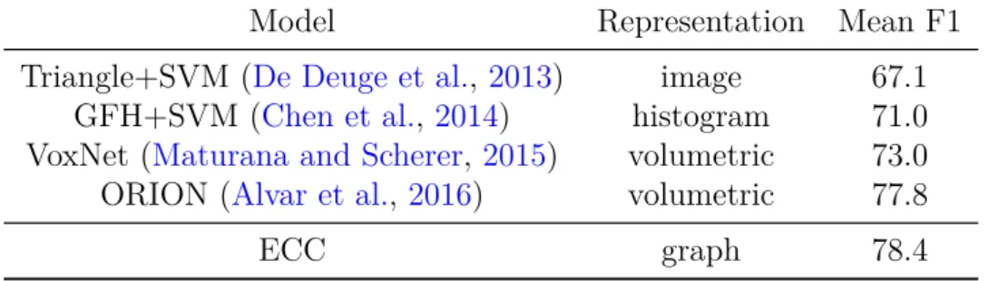
• Nous démontrons les multiples applications de l’ECC/ECC-VV. Le chapitre 3 ex-amine les applications de classification des graphes, en particulier pour les graphes représentant des composés chimiques et pour les graphes de voisinage sur nuages de points. De plus, nous évaluons la performance sur la classification des nœuds dans le contexte de la segmentation sémantique des scènes à grande échelle au chapitre4. ECC est également utilisé comme codeur dans l’autoencodeur moléculaire présenté au chapitre5. En plus d’avoir obtenu l’état de l’art en performance sur plusieurs ensembles de données parmi les méthodes DL aux moments respectifs de publi-cation (NCI1 (Wale et al., 2008), Sydney Urban Objects (De Deuge et al.,2013), Semantic3D (Hackel et al., 2017) et S3DIS (Armeni et al., 2016)), nous étions les premiers à appliquer des convolutions sur graphes pour nuages de points, avec la motivation de préservation de creux et la précision dans le traitement des détails.

• Nous proposons un décodeur de graphes formulé dans le cadre des auto-encodeurs variationnels (Kingma and Welling, 2013) au chapitre 5. Le décodeur produit directement un graphe probabiliste entièrement connecté d’une taille maximale prédéfinie. C’évite quelque peu les problèmes de discrétisation, et utilise la corre-spondance des graphes pendant l’apprentisage afin de tenter de relever le défi du classement indéfini de nœuds. Nous évaluons sur la tâche difficile de la génération de molécules.

(11)

Simonovsky, M. and Komodakis, N. (2016). OnionNet: Sharing Features in Cascaded Deep Classifiers. In Proceedings of the British Machine Vision Conference (BMVC).

Simonovsky, M., Gutiérrez-Becker, B., Mateus, D., Navab, N., and Komodakis, N. (2016). A Deep Metric for Multimodal Registration. In International Conference on Medical

Image Computing and Computer-Assisted Intervention (MICCAI).

Simonovsky, M. and Komodakis, N. (2017). Dynamic Edge-conditioned Filters in Con-volutional Neural Networks on Graphs. In IEEE Conference on Computer Vision and

Pattern Recognition (CVPR).

Landrieu*, L. and Simonovsky*, M. (2018). Large-scale Point Cloud Semantic Segmen-tation with Superpoint Graphs. In IEEE Conference on Computer Vision and Pattern

Recognition (CVPR).

Simonovsky, M. and Komodakis, N. (2018). Towards Variational Generation of Small Graphs. In Sixth International Conference on Learning Representations (ICLR),

work-shop track.

Simonovsky, M. and Komodakis, N. (2018). GraphVAE: Towards Generation of Small Graphs Using Variational Autoencoders. In 27th International Conference on Artificial

Neural Networks (ICANN).

(12)

Acknowledgements

Foremost, I would like to express gratitude to my supervisor Nikos Komodakis for accepting me as his student and securing funding for the whole period, for useful discourses and insights, and especially for giving me the trust and freedom to pursue the research directions I personally found the most interesting and promising. I’m also grateful to the rest of my committee for devoting their precious time to reviewing this thesis and for coming up with many great, thought-provoking questions.

I have experienced very friendly and relaxed atmosphere in my research group, Imagine. In particular, I’m obliged to Renaud Marlet for his warm attitude, negotiating difficult issues and, with the strong support of Brigitte Mondou, for shielding the lab from the outside world. I thank Guillaume Obozinski for his research attitude and didactics, as well as the organization of reading groups, together with Mathieu Aubry. I was also fortunate enough to collaborate on interesting problems with external researchers who taught me a lot along the way. Thank you, Loïc Landrieu, Benjamín Gutiérrez-Becker, Martin Čadík, Jan Brejcha, and Shinjae Yoo.

Uprooted and replanted to France, I was blessed with amazing labmates, many of whom have become good friends of mine. Thank you for all the fun, chats, help, ideas, as well as putting up with GPU exploitation, Benjamin Dubois, Francisco Massa, Laura Fernández Julià, Marina Vinyes, Martin De La Gorce, Mateusz Koziński, Pierre-Alain Langlois, Praveer Singh, Raghudeep Gadde, Sergey Zagoruyko, Shell Hu, Spyros Gidaris, Thibault Groueix, Xuchong Qiu, and Yohann Salaun, as well as Maria Vakalopoulou and Norbert Bus. The past three years would have been lonely and boring without you! Professionally, I’m especially grateful to Sergey, who bootstrapped me into the engineering side of deep learning and taught me lots of good practice, to Francisco for stimulating discussions on everything, and to Shell for keeping me in touch with the theory.

Furthermore, I’m indebted to the community behind Torch, PyTorch, and the whole Python universe. Without all of you, I would still be implementing my first paper now. A very special thanks goes to my dear parents, Dana and Vašek, for their strong belief in education and for their unconditional support through my whole studies; to you I dedicate this thesis. Last but certainly not least, I would like to thank my partner Beata for her patience and tolerance, for enduring our long long-distance relationship, as well as for all the love, moral support, and fun.

(13)

(14)

Chapter 1 Introduction

1.1 Motivation

A graph is a powerful representation of relations between pairs of entities. Its versatility and strong theoretical understanding has resulted in a plethora of use cases across a variety of science disciplines and engineering problems. For example, graphs can naturally be used to describe the structure of chemical compounds, the interactions between regions in the brain, social interactions between people, the topology of three-dimensional models and transportation plans, dependencies of linked web pages, program flows, or knowledge bases. The development of the theory and algorithms to handle graphs has therefore been of major interest.

Formally, a (directed) graph is an ordered pair G = (V, E ) such that V is a non-empty set of vertices (also called nodes) and E ⊆ V × V is a set of edges. Additional information can be attached to both vertices and edges in the form of attributes. A vertex-attributed graph assumes function V → Rdv _{assigning attributes to each vertex. An edge-attributed}

graph assumes function E → Rde _{assigning attributes to each edge.}

The classical graph theory, foundations of which date back to the 18th century, focuses on understanding and analyzing the graph structure and addressing combinatorial problems such as finding mappings, paths, flows or colorings. On the other hand, there has been a lot of research on graph-structured data in the past decades, especially in the signal processing and machine learning communities. In the former, the research has notably brought Fourier transform to irregular domains, giving rise to spectral graph theory and adapting fundamental signal processing operations such as filtering, translation, dilation, or downsampling (Shuman et al., 2013). Usually, a fixed graph is considered with changing data on its nodes. In machine learning, researchers have explicitly made use of graph structures in the data in areas such as graph partitioning

(19)

for clustering, label propagation for semi-supervised learning, manifold methods for dimensionality reduction, graph kernels to describe similarity between different graphs, or graphical models for capturing probabilistic interpretation of data.

In recent years, deep learning (DL) has achieved significant breakthroughs in quantita-tive performance over traditional machine learning approaches in a broad variety of tasks and the field has matured into technologies useful for commercial applications. Promi-nently, a specific class of architecture, called Convolutional Neural Networks (CNNs), has gained massive popularity in tasks where the underlying data representation has a grid structure, such as in speech processing and natural language understanding (1D, temporal convolutions), in image classification and segmentation (2D, spatial convolutions), and in video and medical image understanding (3D, volumetric convolutions) (LeCun et al.,

2015). On the other hand, the case of data lying on irregular or generally non-Euclidean domains has received comparatively much less attention in the community but has become a hot topic during the preparation of this thesis (Bronstein et al.,2017).

Encouraged by the success of DL on grids, in this thesis we study DL architectures for graph-structured data. Specifically, we concentrate on two important primitives: embedding graphs or their nodes into a continuous vector space representation (encoding) and, conversely, generating graphs from such vectors back (decoding). We introduce both problems, their applications and challenges in the following two subsections. Following the DL philosophy of abandoning hand-crafted features for their learned counterparts, our contributions pragmatically build more on accomplished DL methods rather than on past approaches from the machine learning and signal processing community amendable to differentiable re-formulation. The main research question we ask is: How can we

transfer, adapt or generalize DL concepts working well on sequential and image data to graphs?

1.1.1 Embedding Graphs and Their Nodes

One of the central tasks addressed by DL is that of representation learning (Bengio et al.,

2013), i.e. finding a mapping from raw input objects to a continuous vector space of fixed dimensionality Rd_{. Both the mapping and the vector space are also interchangeably called}

embedding or encoding in the literature. The goal is to optimize this mapping so that task-relevant object properties are preserved and reflected in the geometric relationships within the learned embedding space. As an example, in the task of hand-written digit classification, the mapping should capture properties regarding the type of digit, be invariant to those concerning writing style, and strive to make embeddings of images belonging to different classes separable by hyperplanes.

(20)

1.1 Motivation 3

In the case of graphs, we are primarily interested in finding representation of individual nodes as well as of the entire graphs. Usually, information from the local neighborhood of a node is considered in its embedding, while graph embeddings are further computed as some form of aggregation (pooling) of node embeddings. The analogy in deep learning on images is computing pixel-wise features (e.g. for semantic image segmentation) and image-wise features (e.g. for image recognition), respectively. In the case of graphs, there are two kinds of information available. The first is the graph structure as defined by the nodes and edges. The second is the data associated to the graph, i.e. its node and edge attributes. Arguably, a powerful embedding network should be able to exploit as much information as possible.

The ability to compute node embeddings has given rise to many application, such as link prediction (Schlichtkrull et al., 2017), (semi-supervised) node classification in citation networks (Kipf and Welling, 2016a), performing logical reasoning tasks (Li

et al., 2016b), finding correspondences across meshes (Monti et al., 2017) or point

cloud segmentation (Chapter 4). Graph embeddings has also been useful in many tasks, for example measuring similarity of brain networks by metric learning (Ktena

et al., 2017), suggesting heuristic moves for approximating NP-hard problems (Dai

et al., 2017), predicting satisfaction of formal properties in computer programs (Li et al.,

2016b), classifying chemical effects of molecules (Chapter 3) and regressing their physical

properties (Gilmer et al.,2017), or point cloud classification (Chapter 3).

Challenges

The cornerstone of popular network architectures for processing natural images, video or speech is the convolutional layer (LeCun et al., 1998). The translation invariance of the operation, the use of filters with compact support and the application over multiple resolutions fit very well to the statistical properties of such data, namely the stationarity, locality and compositionality.

Besides the fact that the architecture imposes a prior especially suitable for natural images (Ulyanov et al., 2017), another major benefit is the induced strong tying of parameters (weight sharing) across the grid, which greatly reduces the number of free parameters in the network compared to a fully-connected layer (perceptron) while still being able to capture the statistics of real data and enables processing of variable-sized inputs in so-called fully-convolutional style (Long et al., 2015).

Assuming that the stationarity, locality and possibly compositionality principles of representation hold to at least some level in graph data as well, it is meaningful to consider a hierarchical CNN-like architecture for processing it in order to benefit from

(21)

advantages described above. However, the graph domain poses several challenges which make extensions of CNNs to graphs not straightforward. We detail the main challenges below.

Irregular Neighborhoods Unlike on grids, where each node has the same amount of neighbors except for boundaries, nodes in general graphs can have arbitrary number of adjacent nodes. This means that there is no trivial analogy of translation invariance and thus the research objective is to come up with strategies to share parameters of the convolution operator among its applications to different nodes.

Unordered Neighborhoods There is no specific ordering of neighbors of a node, as both nodes and edges are defined as sets. In order to do better that isotropic smoothing, the ability to assign different convolutional weights to different edges is desired. This requires making assumptions or exploiting additional information such as the global structure, degrees of nodes, or edge attributes. On contrary, grids imply a natural ordering of neighborhoods.

Structural Variability In practical scenarios, the graph structure may vary through-out the dataset or may remain fixed, with only the data on nodes changing. The latter is the usual case for applications stemming from the signal processing community, centered around spectral filtering methods (Shuman et al.,2013), and data-mining community, centered around matrix factorization methods (Hamilton et al.,2017a). However, as such methods cannot naturally handle datasets with varying graph structure (for instance meshes, molecules, or frequently updated large-scale graphs), spatial filtering methods have gained on popularity recently. The research question here is to devise explicit local propagation rules and build links to established past work.

Computational Complexity The current DL architectures on grids benefit from heavy parallelism on Graphics Processing Units (GPUs) enabled by well-engineering implementations in popular frameworks such as PyTorch (Paszke et al., 2017) or Ten-sorFlow (Abadi et al., 2015). Unfortunately, the irregular structure of graphs is less amendable to parallelism. The research investigates implementation details such as the use of sparse matrices or other data structures. In addition, for methods based on spectral processing, the naive use of Graph Fourier transform has quadratic complexity in the number of nodes.

(22)

1.1 Motivation 5

1.1.2 Generating Graphs

Deep learning-based generative models have gained massive popularity during several past years, especially in the case of images and text. The principal idea is to collect a large amount of (unannotated) data in some domain and then train a model to generate similar data, i.e. draw samples from a learned distribution closely approximating the true data distribution. As the model has much less parameters than the size of the dataset, it is forced to discover the "essence" of the data rather than to memorize it. Usually, the generative process (also called decoding) is conditioned on a random vector and/or a point from a defined vector space, such as the embedding space of an encoder.

In the case of graphs, we are interested in generating both the structure and associated attributes. There are many applications of such a graph generator, for example creating similar graphs (Bojchevski et al., 2018) or maintaining intermediate representations in reasoning tasks (Johnson, 2017). In an encoder-decoder setup, any kind of input can be encoded to a latent embedding space and then translated to a graph. Possible applications include drug discovery by continuous optimization of certain chemical properties in the latent space (Gómez-Bombarelli et al., 2016), sampling molecules with certain properties (Chapter5) or corresponding to given laboratory measurements (either by conditioning or translation), or simply encoder pre-training in cases where labeled data is expensive.

Challenges

In addition to the challenges usually demonstrated in generative models on grids, such as tricky training (Bowman et al., 2016;Radford et al., 2015), problematic capturing of all distribution modes (Radford et al.,2015) or difficult quantitative evaluation (Theis et al.,

2015), generative models for graph data face several more challenges, detailed below.

Unordered Nodes Data on regular grids provide an implicit ordering of nodes (that is of pixels, characters or words) that is amendable both to step by step generation with autoregressive processes (Bowman et al., 2016; van den Oord et al., 2016) and generation of entire content in a feed-forward network (Radford et al., 2015). However, nodes in graphs are defined as a set and so there is often no clear way how to linearize the construction in a sequence of steps for training autoregressive generators or order nodes in a graph adjacency matrix for generation by a feed-forward network. While there are practical algorithms for approximate graph canonization, i.e. finding consistent node ordering, available (McKay and Piperno,2014), the empirical result ofVinyals et al.

(23)

(2015) that the linearization order matters when learning on sets suggest that it is a priori unclear that enforcing a specific canonical ordering would lead to the best results.

Discrete Nature Similar to text and unlike images, graphs are discrete structures. Incremental construction with autoregressive methods involves discrete decisions, which are not differentiable and thus problematic for gradient-based optimization methods common in DL. In sequence generation, this is typically circumvented by a maximum likelihood objective with so-called teacher forcing (Williams and Zipser, 1989), which allows to decompose the generation into a sequence of conditional decisions and maximize the likelihood of each of them. However, the choice of such a decomposition for graphs is not clear, as we argue above, and teacher forcing is prone the inability to fix its mistakes, resulting in possibly poor prediction performance if the conditioning context diverges from sequences seen during training (Bengio et al., 2015). On the other hand, generation of graphs in a probabilistic formulation can only postpone dealing with non-differentiablity issues to the final step, when the discretized graph has to be output.

Large Graphs The level to which the locality and compositionality principles apply to a particular graph can strongly vary due to possibly arbitrary connectivity - for example, a generator should be able to output both a path and a complete graph. This seems problematic for scaling up to large graphs, as one cannot trivially enforce some form of hierarchical decomposition or coarse-to-fine construction, conceptually similar to using up-sampling operators in images (Radford et al., 2015). This may bring about the necessity to use more parameters while having less regularization implied by the architecture design in the case a feed-forward network. For autoregressive methods, large graphs may make training difficult due to very long chains of construction steps, especially for denser graphs.

1.2 Summary of Contributions

Having charted the two main directions of this thesis and their challenges, we sum-marize our contributions in this section. Most of these contributions were published as "Dynamic Edge-Conditioned Filters in Convolutional Neural Networks on Graphs" at CVPR (Simonovsky and Komodakis, 2017), as "Large-scale Point Cloud Semantic Segmentation with Superpoint Graphs" at CVPR (Landrieu and Simonovsky, 2018), as "Towards Variational Generation of Small Graphs" at ICLR workshop track (Simonovsky

(24)

1.2 Summary of Contributions 7

Variational Autoencoders" at ICANN (Simonovsky and Komodakis, 2018a). Martin Simonovsky is the leading author in all publications with the exception of Landrieu and

Simonovsky(2018), where the contribution is equally shared with Loïc Landrieu.

• We propose Edge-Conditioned Convolution (ECC) in Chapter3, a novel convolution-like operation on graphs performed in the spatial domain where filters are condi-tioned on edge attributes (discrete or continuous) and dynamically generated for each specific input graph. This allows the algorithm to exploit enough structural information in local neighborhoods so that our formulation can be shown to gen-eralize discrete convolution on grids. Due the application in spatial domain, the method can work on graphs with arbitrary and varying structure. In Chapter4, we integrate ECC into a recurrent network and reduce its memory and computational requirements, reformulating it as ECC-VV.

• We introduce SuperPoint Graph (SPG) in Chapter 4, a novel point cloud repre-sentation with rich edge attributes encoding the contextual relationship between object parts. Based on this representation, we are able to apply deep learning in the form of ECC/ECC-VV on large-scale point clouds without major sacrifice in fine details.

• We demonstrate multiple applications of ECC/ECC-VV. Chapter 3 investigates graph classification applications, in particular for graphs representing chemical compounds and for neighborhood graphs of point clouds. Further, we evaluate the performance on node classification in the context of semantic segmentation of large-scale scenes in Chapter4. ECC is also used as encoder in the molecular autoencoder presented in Chapter 5. Besides having obtained the state of the art performance on several datasets among DL methods at the respective times of publication (NCI1 (Wale et al., 2008), Sydney Urban Objects (De Deuge et al.,

2013), Semantic3D (Hackel et al.,2017) and S3DIS (Armeni et al., 2016)), we were the first to apply graph convolutions to point cloud processing, with the motivation of preserving sparsity and presumably fine details.

• We propose a graph decoder formulated in the framework of variational autoen-coders (Kingma and Welling, 2013) in Chapter 5. The decoder outputs a proba-bilistic fully-connected graph of a predefined maximum size directly at once, which somewhat sidesteps the issues of discretization, and uses graph matching during training in order to attempt to overcome the challenge of undefined node ordering. We evaluate on the difficult task of molecule generation.

(25)

Besides the central topic of deep learning on graphs, we have conducted research along several other lines within the duration of the thesis. These activities have resulted in two publications, which are not part of this manuscript and which we therefore briefly summarize below:

• In the domain of medical image registration, we proposed a patch similarity metric based on CNNs and applied it to registering volumetric images of different modal-ities. The key insight was to exploit the differentiability of CNNs and directly backpropagate through the trained network to update transformation parameters within a continuous optimization framework. The training was formulated as a clas-sification task, where the goal was to discriminate between aligned and misaligned patches. The metric was validated on intersubject deformable registration on a dataset different from the one used for training, demonstrating good generalization. In this task, we outperformed mutual information by a significant margin. The work was done in collaboration with Benjamín Gutiérrez-Becker from TU Munich as a second author and was published as "A Deep Metric for Multimodal Registration" at MICCAI 2016 (Simonovsky et al.,2016).

• For retrieval scenarios in computer vision, we proposed a way of speeding up evaluation of deep neural networks by replacing a monolithic network with a cascade of feature-sharing classifiers. The key feature was to allow subsequent stages to add both new layers as well as new feature channels to the previous ones. Intermediate feature maps were thus shared among classifiers, preventing them from the necessity of being recomputed. As a result demonstrated in three applications (patch matching, object detection, and image retrieval), the cascade could operate significantly faster than both monolithic networks and traditional cascades without sharing at the cost of marginal decrease in precision. The work was published as "OnionNet: Sharing Features in Cascaded Deep Classifiers" at BMVC 2016 (Simonovsky and Komodakis, 2016).

1.3 Outline

In this section we summarize the chapters of the thesis and relate them to each other.

Chapter 2: Background and Related Work This chapter provides the background

and overviews related and prior work on graph-structured data analysis. Both classic and deep learning-based methods are covered. Further discussions of related and contemporary work are also provided within each core chapter.

(26)

1.3 Outline 9

Chapter 3: Edge-Conditioned Convolutions This chapter introduces the main

workhorse of this thesis, graph convolutions able to process continuous edge at-tributes. The method is applied to small-scale point cloud classification and biological graph datasets.

Chapter 4: Large-scale Point Cloud Segmentation This chapter applies ECC to

the the problem of segmentation of large areas, such as streets or office blocks, by working on homogeneous segments instead of individual points.

Chapter 5: Generation of Small Graphs This chapter introduces a graph

autoen-coder based on ECC and graph matching with an application to drug discovery, where novel molecules need to be sampled.

Chapter 6: Conclusion This chapter reflects on the contributions of the thesis and

(27)

(28)

Chapter 2 Background and Related Work

This chapter provides background and overview of related and prior work on (sub)graph embedding techniques. After introducing our notation in Section2.1, we dive into classical (non-deep) signal processing on graphs in Section2.2, which is mostly formulated in the spectral domain. This knowledge is then useful for the overview of spectral deep learning-based convolution methods, introduced in Section2.3. We mention their shortcoming and move on to review the progress in spatial convolution methods in Section2.4, also in relation to the contributions of this thesis. To make the picture complete, we briefly mention non-convolutional approaches for embedding, namely direct embedding and graph kernels, in Section 2.5.

While this thesis focuses exclusively on graphs, it is worth to mention the progress made in (deep) learning on manifolds. Whereas the fields of differential geometry and graph theory are relatively distant, both graphs and manifolds are examples of non-Euclidean domains and the approaches for (spectral) signal processing and for convolutions in particular are closely related, especially when considering discretized manifolds - meshes. We refer the interested reader to the nice survey paper ofBronstein

et al.(2017) for concrete details.

2.1 Attributed Graphs

Let us repeat and extend graph-related definitions from the introduction. A directed graph is an ordered pair G = (V, E ) such that V is a non-empty set of vertices (also called nodes) and E ⊆ V × V is a set of edges (also called links). Undirected graph can be defined by constraining the relation E to be symmetric.

It is frequently very useful to be able to attach additional information to elements of graphs in the form of attributes. For example, in graph representation of molecules,

(29)

vertices may be assigned atomic numbers while edges may be associated with information about the chemical bond between two atoms. Concretely, a vertex-attributed graph assumes function F : V → Rdv _{assigning attributes to each vertex. An edge-attributed}

graph assumes function E : E → Rde _{assigning attributes to each edge. In the special}

case of non-negative one dimensional attributes E → R+_{, we call the graph weighted.} Discrete attributes E → N can be also called types.

In addition to attributes, which are deemed being a fixed part of the input, we introduce mapping H : V → Rd _{to denote vertex representation due to signal processing}

or graph embedding algorithms operating on the graph. This mapping is called signal (especially if d = 1) or simply data. Often, vertex attributes F may be used to initialize

H. The methods for computation of H will constitute a major part of discussion in this

thesis.

Finally, assuming a particular node ordering, the graph can be conveniently described in matrix, resp. tensor form using its (weighed) adjacency matrix A, signal matrix H, node attribute matrix F and edge attribute tensor E of rank 3.

2.2 Signal Processing on Graphs

Here we briefly introduce several concepts regarding multiscale signal filtering on graphs, which are the basis of spectral graph convolution methods presented in Section 2.3 and also used for pooling in Chapter 3.

Mathematically, both a one-dimensional discrete-time signal with N samples as well as a signal on a graph with N nodes can be regarded as vectors f ∈ RN_{. Nevertheless,}

applying classical signal processing techniques on the graph domain would yield subopti-mal results due to disregarding (in)dependencies arising from the irregularity present in the domain.

However, the efforts to generalize basic signal processing primitives such as filtering or downsampling faces two major challenges, related to those mentioned in Section1.1.1:

Translation While translating time signal f (t) to the right by a unit can be expressed

as f (t − 1), there is no analogy to shift-invariant translation in graphs, making the classical definition of convolution operation (f ∗ w)(t) :=R

τg(τ )w(t − τ )dτ not

directly applicable.

Coarsening While time signal decimation may amount to simply removing every other

point, it is not immediately clear which nodes in a graph to remove and how to aggregate signal on the remaining ones.

(30)

2.2 Signal Processing on Graphs 13

In the following subsections, we describe three core concepts developed by the signal processing community: graph Fourier transform, graph filtering operations and graph coarsening operations. We refer to the excellent overview papers ofShuman et al. (2016,

2013) for a broader perspective as well as details.

2.2.1 Graph Fourier Transform

Assuming undirected finite weighted graph G on N nodes, let A be its weighted adjacency matrix and D its diagonal degree matrix, i.e. Di,i = PjAi,j. The central concept in

spectral graph analysis is the family of Laplacians, in particular the unnormalized graph Laplacian L := D − A and the normalized graph Laplacian L := D−1/2(D − A)D−1/2 =

I − D−1/2AD−1/2. Intuitively, Laplacians capture the difference between the local average of a function around a node and the value of the function at the node itself. We denote {ul} the set of real-valued orthonormal eigenvectors of a Laplacian and {λl} the set

of corresponding eigenvalues. Interestingly, Laplacian eigenvalues provide a notion of frequency in the sense that eigenvectors associated with small eigenvalues are smooth and vary slowly across the graph (i.e. , the values of an eigenvector at two nodes connected by an edge with large weight are likely to be similar) and those associated with larger eigenvalues oscillate more rapidly.

The analogy between graph Laplacian spectra and the set of complex exponentials, which are eigenfunctions of the classical Laplacian operator on Euclidean space and provide the basis for the classical Fourier transform, is the motivation for introducing an analogy to Fourier transform on graphs. The graph Fourier transform ˆf of signal f ∈ RN _{on the nodes of G is defined as the expansion in terms of Laplacian eigenvectors}

ˆ

f (λl) :=< f , ul >= PN −1i=0 f (i)ul(i) and the inverse graph Fourier transform is then

computed as f (i) =PN −1

l=0 f (λˆ l)ul(i).

We remark that extensions to directed graphs are complicated (Sardellitti et al.,2017). Also, handling of discrete or multidimensional edge attributes is not supported by the framework, to the best of our knowledge, although one way of circumventing the latter might be to simultaneously consider multiple graphs with the same connectivity but different edge weights, each graph corresponding to a single real, non-negative attribute dimension.

(31)

2.2.2 Signal Filtering

Using graph Fourier transform, a signal can be equivalently represented in the spatial (node) domain and in the graph spectral domain. Thus, as in classical signal processing,

the signal can be filtered in either of the domains.

Graph spatial filtering amounts to expressing the filtered signal g at node i as a

linear combination of the input signal f at nodes within its K-hop local neighborhood NK: g(i) = Bi,if (i) +Pj∈NK(i)Bi,jf (j) with filter coefficients matrix B. While this is a

(spatially) localized operation by design, it requires specifying O(N2_{) coefficients unless} some form of regularity is assumed.

Graph spectral filtering follows the classical case, where filtering corresponds to

multiplication in the spectral domain, i.e. the amplification or attenuation of the set of basis functions. It is defined as ˆg(λl) = ˆf (λl) ˆw(λl). This suggests a way of generalizing

the convolution operation on graphs by the means of spectral filtering as

g(i) = (f ∗Gw)(i) := N −1 X l=0 N −1 X j=0 f (j) ˆw(λl)ul(i)ul(j) (2.1)

It is important to remark that spectral filter coefficients ˆw are specific to the given

graph, resp. the particular choice of its Laplacian eigenvectors.

Using the full range of N coefficients makes spectral filtering perfectly localized in the Fourier domain but not localized in the spatial domain due to uncertainty principle, its extension to graphs first developed by Agaskar and Lu (2013) but still considered an open problem. However, this property is usually undesired in practice. The popular remedy is to make the filter spectrum "smooth" by ordering the eigenvectors according to their eigenvalues and expressing coefficients as continuous function of only a few free parameters. To make the link between spectral and spatial filtering, it is interesting to parameterize the spectral filter as order K polynomial ˆw(λl) = PK−1k=0 akλkl with

coefficients a. It can be shown that this construction corresponds to a spatial filter on K-hop neighborhood for a particular choice of Bi,j :=PK−1k=0 akLki,j (Shuman et al.,

2013). Thus, polynomial spectral filters are exactly localized within a certain spatial neighborhood and have only a limited number of free parameters, independent of N , which is beneficial for any learning task, as shown byDefferrard et al. (2016).

Nevertheless, even in the localized case the cost of filtering a graph signal in the spectral domain is an O(N2_{) operation due to the multiplications with Fourier basis} in Equation 2.1. Fortunately, approximation methods have been developed for fast filtering in the case of sparse graphs, where the filter is formulated directly in the spatial domain as a polynomial in L that can be evaluated recursively, leading to computational

(32)

2.2 Signal Processing on Graphs 15

complexity linear with the number of edges. A popular choice for the polynomial is truncated Chebyshev expansion (Shuman et al., 2011). Note that this does not require an explicit computation of the Laplacian eigenbasis.

Building banks of filters localized both in space and frequency has been intensively studied in the context of graph wavelets and we refer to the review in (Shuman et al.,

2013) for more details. Wavelet coefficients can serve as descriptors for classification or matching tasks in non-deep machine learningMasoumi and Hamza (2017).

2.2.3 Graph Coarsening

In the Euclidean world, multiresolution representation and processing of signals and images with techniques such as pyramids, wavelets or CNNs has been very successful. Finding a similar concept for graphs is therefore of interest. The task of graph coarsening is to form a series of successively coarser graphs G(s) _{= (V}(s)_{, E}(s)_{) from the original graph}

G = G(0)_{. Coarsening typically consists of three steps: subsampling or merging nodes,} creating the new edge structure E(s) _{and weights (so-called reduction), and mapping the} nodes in the original graph to those in the coarsened one with C(s) _{: V}(s−1) _{→ V}(s)_{. In} many practical cases, a desirable property of coarsening is to halve the number nodes at each level while clustering nodes connected with large weights together. For unweighted bipartite graphs, there is a natural way of coarsening by sampling "every other node". But the task is more complex for other cases, which has led to creation of various algorithms.

One line of work is based on partitioning the set of nodes into clusters and representing these with a single node in the coarsened graph. For example, Graclus (Dhillon et al.,

2007) greedily merges pairs of nodes based on clustering heuristics such the normalized cut

Ai,j(1/Di,i+1/Dj,j), which is efficient but not optimal. The union of the neighborhoods of

the two original nodes becomes the neighborhood of the merged node, leading to decreased sparsity of the coarsened graphs. This algorithm is used for pooling inDefferrard et al.

(2016).

Another line of work keeps a strict subset of original nodes during the coarsening steps. For example, Shuman et al. (2016) select the nodes to keep based on the sign of entries in the eigenvector associated with the largest Laplacian eigenvalue (frequency), which can be computed efficiently by the power method. The sign is shown to behave intuitively on bipartite graphs, such as grids or trees. Kron reduction (Dörfler and Bullo,

2013) is suggested as a method of choice to compute the coarsened Laplacian, defned as the Schur complement of the original Laplacian with respect to the removed node indices. It offers many nice properties but leads to a decrease in sparsity, which can be amended by postprocessing with spectral sparsification (Spielman and Srivastava, 2011),

(33)

among others. This randomized algorithm samples edges according to the probability of the edge appearing in a random spanning tree of the graph, thus mostly removing those structurally unimportant edges. We use this pipeline for pooling operation later in Chapter 3.

Finally, let us remark that graph resolutions generated in this fashion are completely independent of any signals residing on the graph nodes.

2.3 Spectral Graph Convolutions

In this section, we review how the deep learning community have applied spectral signal processing methods, introduced above, to learning tasks. The characteristic feature of these methods is the explicit use of graph Laplacian in the convolution operation.

In their pioneering work, Bruna et al. (2013) learned filters using the formulation of spectral convolution in Equation 2.1. This can be conveniently expressed in matrix form as ht+1 _{= U ΘU}T_ht_{, where U is the column-wise concatenation of Laplacian eigenvectors}

{ul}, Θ is a diagonal matrix of filter coefficients and ht and ht+1 is the input and output

signal vector, respectively. Each spectral filter Θ is parameterized as B-spline with the number of free parameters independent of graph size N to reduce the risk of overfitting and to make filters smooth and therefore localized in space. In addition, high frequency eigenvectors may be discarded for better computational efficiency of Fourier transform, which nevertheless remains quadratic in the number of eigenvectors. By using multiple filters per layer, stacking multiple convolutional layers and considering coarsened graphs created by agglomerative clustering, Bruna et al.were the first to present a graph analogue of classic CNNs.

Defferrard et al.(2016) later proposed an efficient spectrum-free method by formulating

spectral filters as Chebyshev polynomials, as briefly introduced in Section 2.2.2above. The filtering is evaluated directly in the spatial domain on a K-hop neighborhood and can be written in matrix notation as ht+1 ₌PK−1

k=0 θkTk( ˜L)ht where θ is a vector of K

parameters and Tk is Chebyshev polynomial of order k evaluated at the scaled Laplacian

˜

L := 2L/ max λ − I. Coarsening for pooling purposes is done by Graclus (Dhillon et al.,

2007), which does not require computation of the spectrum either.

This approach was further simplified by Kipf and Welling (2016a), who proposed its first-order approximation in spatial domain as ht+1 _{= θ(I − ˆ}_L)ht _{where θ is a scalar}

parameter and ˆL is the Laplacian of the adjacency matrix with added self-connections

ˆ

A = A + I. In effect, this model corresponds to simply taking average of neighboring

(34)

2.4 Spatial Graph Convolutions 17

Note that despite the spatial evaluation of spectral methods, model parameters are still tied to the particular Laplacian and the trained networks may not generalize to other graph structures; this has been empirically demonstrated byMonti et al. (2017) for the model of Defferrard et al.(2016). Yi et al.(2017) embarked on addressing this for the case of 3D shapes represented as meshes by mapping the spectral representation of signal on an input graph to a predefined canonical graph, in the context of which filters are learned. The mapping is a linear transformation predicted by a special network from the voxelized eigenbasis of the input mesh. The authors leverage duality in functional maps between spatial and spectral correspondences and use ground truth correspondences between shapes to initialize the training, which they described as extremely challenging.

Finally, let us recap that spectral methods have been shown to work on undi-rected graphs only, as the adaptation of Laplacian to diundi-rected graphs is not straightfor-ward (Sardellitti et al., 2017). An interesting way of circumventing this was proposed by

Monti et al.(2018), who exploit the concept of motifs (small subgraphs) to construct a

symmetric motif-induced adjacency matrix based on a non-symmetric adjacency matrix by counting the number of times an edge takes part in a set of canonical motifs.

2.4 Spatial Graph Convolutions

We have seen above that while the spectral construction is theoretically well motivated, there are obstacles in going beyond a single undirected graph structure. The spatial construction, on the other hand, may not have these limitations, though its designs are perhaps less principled. This section overviews the development in spatial construction methods for graph convolution and is closely related to the contributions presented in Chapters 3and 4.

Let Ht_{∈ R}N ×dt be dt-dimensional signal matrix at N nodes. Spatial graph convolution amounts to expressing the output signal H_it+1 _{∈ R}dt+1 at node i as a function of the input signal H_jt_{∈ R}dt at nodes j within its K-hop local neighborhood. Scarselli et al.

(2009) proposed one of the first propagation models M , which (somewhat ironically) is arguably also the most general one: it may depend in an arbitrary way on the signals H, as well as edge and node attributes E and F within an arbitrary neighborhood N (i), formally written as

(35)

To account for the fact that neighboring nodes are typically unordered, the general form is then restricted to pairwise potentials with an aggregation over direct neighbors as

H_it+1= u(Fi, X j∈N (i)

m(H_jt, Fi, Fj, Ej,i). (2.3)

The functions m and u are designed to be contractive operators, the whole network is treated as a dynamical system and solved for fixed point solution for H from any initial state in its forward pass1_{. No concept of graph-level output or graph coarsening was}

mentioned.

Recently, many graph convolution variants have appeared in the community. To make their comparison easier,Gilmer et al. (2017) suggested Message Passing Neural Network (MPNN) family fitting the vast majority of models of that time. It is a modified version of Scarselli’s Equation2.3, where a) node labels are used for initializing node state H0 rather than for propagation and b) states of both the source and the destination node can be used for propagation. Concretely,Gilmer et al. (2017) use the message function

m and the node update function u in the following way:

M_it+1= X j∈N (i) mt(Hit, Hjt, Ej,i) H_it+1= ut(Hit, M t+1 i ) (2.4)

These function define a recurrent neural network (RNN) where the state is processed over several iterations (time steps) t = 1 . . . T . At each iteration t, the update function takes its hidden state H_it and updates it with M_it+1, which is the aggregation of messages

mt incoming from each neighbor. Finally, a readout function is defined to aggregate

final node states into a graph-level state. We will use this framework (without the readout function, for simplicity) to chronologically review interesting related works in the following. Note that the list is far from being exhaustive, as there has been an explosion of many very closely related or sometimes even identical models in the community recently.

Bruna et al. (2013) suggested a spatial method, in addition to his spectral model

described in Section 2.3. Here, mt : Wt,j,iHjt and ut : ReLU(Mit+1) with an

edge-specific matrices of parameters W . The disadvantage of no weight sharing is a large number of parameters and no generalization over different graphs.

1_{It would be a very interesting exercise to implement this approach in a current deep learning} framework and benchmark it against contemporary RNN-based graph convolution methods. Li et al.

(2016b) provide a theoretical insight that contraction is expected to attenuate the effect of long-range

(36)

2.4 Spatial Graph Convolutions 19

Duvenaud et al. (2015) proposed message passing function mt: Hjt and update

func-tion ut : tanh(Wt,deg(i)Mit+1) with node-degree specific matrices of parameters

W . The signal is passed over edges indiscriminately (nevertheless, there are weak

constraints for possible edge types and node degree in their specific context of molecular fingerprints).

Mou et al. (2016) proposed convolution operation on ordered trees, where the weights

linearly depend on the position of a node within a triangular window containing the parent node and children, mt: (ηj1W1+ η2jW2+ η3jW3)Hjt+ b and ut: tanh(Mit+1),

where η are barycentric coordinates and W , b are learnable parameters.

Li et al. (2016b) introduced support for discrete edge types and successful RNN layers,

such as the Gated Recurrent Unit (Cho et al.,2014a), by having mt: WEj,iHjt and

ut : GRU(Hit, M t+1

i ), where W are edge-type and edge-direction specific weight

matrices.

Kearnes et al. (2016) developed a model where both nodes and edges hold

hid-den representations updated in an alternating fashion. Formally mt : Ej,it , ut :

ReLU(W2[ReLU(W1H_it), M_it+1]) and E_j,it+1 = ReLU(W5[ReLU(W3E_j,it ), ReLU(W4[H_it, H_jt])]) where [·] denotes concatenation and W weight matrices.

Battaglia et al. (2016) implemented the general version of MPNN in Equation 2.4

with mt and ut as multi-layer perceptrons. This stands out from most other

approaches by not explicitly decomposing message passing into a form of multipli-cation of Ht

j with some weights. While the formulation has been proposed before

Gilmer et al.(2017), it has been demonstrated only as a single convolutional layer

on fully connected graphs with discrete edge attributes.

Schütt et al. (2017) replaced the usual matrix-vector multiplication with

element-wise multiplication in lower-dimensional space, leading to message function mt :

tanh(W1_((W2_Ht

j + b1) ⊙ (W3Ej,i + b2)) and ut : Hit + M t+1

i where W and b

are learnable parameters. Later in (Schütt et al., 2017), the authors allowed for handling continuous edge attributes, leading to basically the same message function as in Gilmer et al.(2017).

Monti et al. (2017) , building on their previous work on learning on manifolds and

meshes, proposed a Gaussian mixture model for message passing conditioned on continuous edge attributes. The model with K mixture components can be written as mt : w(Ej,i)Hjt with edge weighting function w,