Research Article
High-Resolution Wellbore Temperature Logging Combined with
a Borehole-Scale Heat Budget: Conceptual and Analytical
Approaches to Characterize Hydraulically Active Fractures and
Groundwater Origin
Guillaume Meyzonnat ,
1Florent Barbecot,
1José A. Corcho-Alvarado,
2Antoine Tognelli,
3Hermann Zeyen,
4Alexandra Mattei,
1,5and Renald McCormack
61Department of Earth and Atmospheric Sciences, Geotop-UQAM, Montr´eal, QC, Canada 2Spiez Laboratory, Federal Office for Civil Protection, Spiez, Switzerland
3CEA, DAM, DIF, F-91297 Arpajon, France
4Department of Earth Sciences, GEOPS Laboratory, Paris-Saclay University, Paris-Sud University, CNRS, Orsay, France 5MINES Paris Tech, Paris, France
6Envir’Eau-Puits Inc., Saint-Nicolas, QC, Canada
Correspondence should be addressed to Guillaume Meyzonnat; [email protected] Received 29 June 2017; Revised 18 October 2017; Accepted 20 February 2018; Published 3 April 2018 Academic Editor: Walter A. Illman
Copyright © 2018 Guillaume Meyzonnat et al. This is an open access article distributed under the Creative Commons Attribution License, which permits unrestricted use, distribution, and reproduction in any medium, provided the original work is properly cited.
This work aims to provide an overview of the thermal processes that shape wellbore temperature profiles under static and dynamic conditions. Understanding of the respective influences of advection and conduction heat fluxes is improved through the use of a new heat budget at the borehole scale. Keeping in mind the thermal processes involved, a qualitative interpretation of the temperature profiles allows the occurrence, the position, and the origin of groundwater flowing into wellbores from hydraulically active fractures to be constrained. With the use of a heat budget developed at the borehole scale, temperature logging efficiency has been quantitatively enhanced and allows inflow temperatures to be calculated through the simultaneous use of a flowmeter. Under certain hydraulic or pumping conditions, both inflow intensities and associated temperatures can also be directly modelled from temperature data and the use of the heat budget. Theoretical and applied examples of the heat budget application are provided. Applied examples are shown using high-resolution temperature logging, spinner flow metering, and televiewing for three wells installed in fractured bedrock aquifers in the St-Lawrence Lowlands, Quebec, Canada. Through relatively rapid manipulations, thermal measurements in such cases can be used to detect the intervals or discrete positions of hydraulically active fractures in wellbores, as well as the existence of ambient flows with a high degree of sensitivity, even at very low flows. Heat budget calculations at the borehole scale during pumping indicate that heat advection fluxes rapidly dominate over heat conduction fluxes with the borehole wall. The full characterization of inflow intensities provides information about the distribution of hydraulic properties with depth. The full knowledge of inflow temperatures indicates horizons that are drained from within the aquifer, providing advantageous information on the depth from which groundwater originates during pumping.
1. Introduction
Aquifer hydraulic properties are most commonly determined through pumping and slug tests. These techniques provide fast and reliable measurements of mean transmissivity and effective porosity, which often yield sufficient information
to manage groundwater resources in terms of productivity. However, for applications where solute transport processes cannot be neglected (i.e., wellhead protection area delin-eation, contaminated site remediation), the knowledge of mean hydraulic parameters alone is insufficient, and ground-water flow paths need to be assessed. Hydrogeologists always
Volume 2018, Article ID 9461214, 19 pages https://doi.org/10.1155/2018/9461214
have to deal with a certain degree of spatial heterogeneity, because aquifer architectures originate from complex geolog-ical processes (i.e., sedimentology, tectonics), which generate heterogeneous [1] and scale-dependent patterns [2]. Despite the heterogeneous nature of aquifers, the use of borehole logging techniques to address this heterogeneity remains uncommon. For instance, pumping tests usually carried out for drinking water supply wells do not typically address the vertical variability of the production zones within the boreholes [3]. Since the most common borehole logging technique, known as the packer test, is more difficult to implement, more time-consuming, and thus more expensive than usual pumping tests, the vertical investigation of aquifer heterogeneities is still rare in hydrogeological surveys.
The heterogeneous nature of aquifers has been investi-gated and highlighted worldwide. In the Canadian context of this study, examples dealing with aquifer heterogeneity have been provided for both granular [4] and fractured [5] matrices. Nastev et al. [6] described the lognormal decrease of hydraulic conductivities with depth in postglacial fractured bedrock in Quebec, Canada. Recent regional groundwater characterizations, also carried out in Quebec, between 2008 and 2015, included the investigation of vertical bedrock fracturing patterns. These generally showed no correlation between well productivity and type of bedrock formation [7–9]. Packer tests and acoustic televiewing performed by Carrier et al. [7] showed that decreasing fracture densities are generally associated with decreasing hydraulic conductivities with depth. However, these results have high standard devia-tions, revealing strong vertical heterogeneities from one well to another. Indeed, packer tests performed for some wells in the same period [8, 9] did not reveal systematic decreases in bedrock fracturing with depth.
Other borehole logging techniques have garnered the attention of hydrogeologists over the last two decades. For instance, tracer experiments allow fluid velocities [10] or concentration dilution [11] to be measured following the injection of a tracer into boreholes during pumping, or tracer breakthrough in boreholes neighboring the injection well to be measured [12]. Spinner [13] or electromagnetic [14, 15] flowmeters allow water velocities to be measured very efficiently and directly inside the borehole with high spatial resolution. Such fluid velocity measurements inside boreholes during pumping allow the vertical distribution of the hydraulic properties of the surrounding rocks to be determined [13]. For the same application, but under low flow conditions, heat pulse flowmeters [15, 16] are especially useful to measure ambient borehole flow. Temperature logging in boreholes is another type of investigation technique. Appli-cations specifically dedicated to hydrogeology make use of temperature logging in boreholes to estimate recharge rates [17–19], to trace local [20, 21] or regional [22] groundwater flows, or to infer the lateral heterogeneity of hydraulic properties for a section of an aquifer [23]. These applications typically address large-scale heat transport processes within the subsurface and/or involve heat transport processes over relatively long time scales.
At the borehole scale, high-resolution temperature pro-filing is of particular interest in hydrogeology, and its use
has become more frequent over the last decade, coinciding
with temperature sensor resolution improvement to 0.001∘C.
Hydrogeological information obtained from recent passive and/or active temperature measurement techniques [24, 25] are now capable of competing with other, more conventional investigation techniques (e.g., involving hydraulic packer tests or solute tracing) to provide valuable information about aquifer hydraulic and fracturing structure, used to infer groundwater flow paths.
Passive temperature measurements consist of logging temperature in a wellbore without introducing a heat source, so that obtained profiles only depend on natural hydrogeolo-gical conditions, thermal properties of the rock, and/or aquifer solicitation through pumping. For instance, the verti-cal distribution and interconnectivity of fractures in well-bores can be well-described by coupling flow and passive temperature measurements. Such examples are given by Chatelier et al. [26] and Le Borgne et al. [27], who have explicitly pointed out the advantage of combining passive temperature and flowmeter logs, where the passive tempera-ture log gives the precise depth at which inflow occurs, and the flow log gives a precise measurement of the flow rate in the interval between inflow and outflow zones. Discussions of groundwater origin from identified fractures are also found in the literature. One such example is also provided by Chatelier et al. [26], by coupling passive temperature measurement and flow logs with elaborate in situ data. Other recent technical advances make it possible to measure instantaneous tem-perature profiles using optical fiber. This technology is often implemented with an active measurement of temperature by heating a section or the entire length of the water column. Pehme et al. [28] used active temperature measurements to detect lateral ambient flow through hydraulically active frac-tures by measuring the thermal recovery of the water column in the borehole after it was heated. In another example, Bense et al. [29] used a coaxial system of heating cable and optical fiber and then used the variation in temperature profiles during pumping to calculate the depth-flow distribution in wellbores.
Although these latter active technologies allow direct quantitative results, their setup remains rather delicate and time-consuming for in situ applications. Moreover, the effec-tiveness of the method is not guaranteed in all in situ cases, because the resolution of optical fiber temperature
measurements (±0.5∘C, or at best ±0.02∘C with the use of
the calibration baths) is still low compared with those of the
current thermistors (±0.001∘C), which are preferentially used
for passive measurements. Thermal numerical modelling has been used by Klepikova et al. [30] and Klepikova et al. [31] to present the concepts and numerical methods behind the inversion of temperature profiles to flow profiles in wellbores, thus using the temperature probe as a high-resolution flowmeter. Previous work has made use of thermal analytical models, especially in the case of (low) ambient flows in wellbores for fractured media. An explicit thermal analytical solution considering a semi-infinite plane geome-try was provided by Drury and Jessop [32] to model transient temperature shifts within the aquifer with increasing distance from the active fracture intercepting the wellbore. With an
application for ambient inflow, which flows through the wellbore, Ge [33] proposed a theoretical model to estimate both fluid flow velocity and temperature for a given inflow. Previous work has focused on experiments under thermal steady-state conditions during pumping and was generally applied at depth or at locations where the geothermal gradient is linear.
This study investigates the vertical distribution of hyd-raulic properties in fractured bedrock wells using flow meter-ing and televiewmeter-ing, but with a main focus on temperature borehole logging. As cited above, numerous works have already highlighted the pertinence of temperature logging to identify the occurrence and the positions of productive zones in wellbores. Through the introduction of a new heat budget model, this work aims to enhance the qualitative
interpretation of depth-temperature profiles against
advection and conduction fluxes at the borehole scale, across a range of static and dynamic conditions in fractured aquifers. The second objective is to enhance the potential of passive temperature logging to quantify flow and the temperature of inflows into boreholes with the use of a heat budget. Previous analytical models found in the literature typically allowed calculations for only a limited number of fractures (i.e., one or two fractures at best, in the case of ambient flows) and did not attempt to model the complete depth-temperature profile when several inflows occurred and mixed in the wellbore. The heat budget proposed in this work aims to model depth-temperature profiles for the entire wellbore length, for several inflows that mix in the borehole, and depending on pumping conditions (duration and discharge intensity). Simultaneous temperature measurement and flow metering are applied within the heat budget to quantify information about the origin of several groundwater inflows based on their temperature. The use of this analytical procedure is also theoretically investigated to test its potential to quantify both flow and temperature of inflows in wellbores through the single logging of depth-temperature profiles.
The following abbreviations are used throughout the text for brevity: the temperature of the water column measured
in the borehole under ambient (TS) and under dynamic (i.e.,
pumping) (TD) conditions; the temperature of groundwater
discharging into the borehole at depth (Ti), originating from
a discrete or distributed interval of hydraulically active
frac-ture(s); and the temperature of the aquifer (TA), depending
on depth as function of geothermal heat flux, seasonal and climatic variation of the soil surface temperature, regional groundwater circulation, and recharge fluxes, but excluding the influence of fluid advection due to the presence of a wellbore or the pumping thereof.
2. Materials and Methods
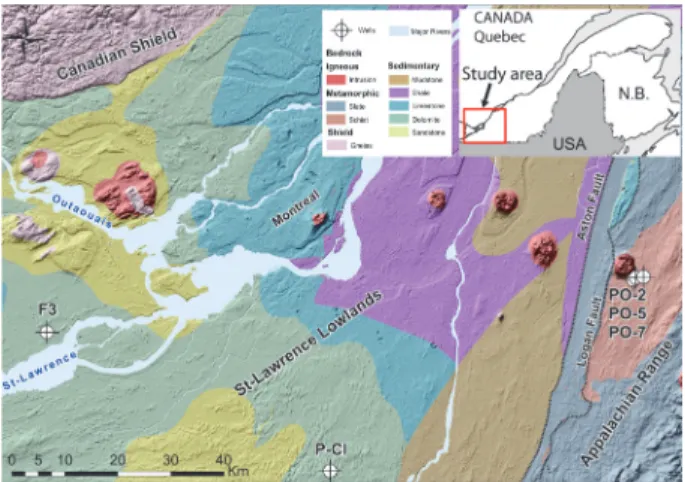
2.1. Site Description. The study area is located in southern
Quebec, within two geological regions that correspond to the St. Lawrence Platform and the Appalachian Mountains (Fig-ure 1). The Ordovician geological units of the St. Lawrence Platform are of sedimentary origin and consist of thick sequences of sandstone of the Potsdam Group, dolomite of the Beekmantown Group, limestone of the Chazy, Black
Figure 1: Location of wells in the current study and geological map.
River, and Trenton Groups, Utica shales, and mudstones of the Queenston Group. In the eastern part of the study area, the Appalachian range corresponds to complex, imbricated metamorphic thrust sheets produced during the Taconian Orogeny: slates with a bedded shaly matrix containing chaotic blocks of cherts, sandstone, and dolomitic schists. These geological units are represented in Figure 1 as a simplified version of the detailed mapping by Globensky [34]. The geomorphology of Quebec is marked by glaciation-deglaciation phases, with unconsolidated sediments of glacial and postglacial origin overlying the fractured bedrock. The complex stratigraphy of the unconsolidated sediment largely controls the hydrogeological context of the underlying frac-tured bedrock aquifers. In such a glacial geomorphological context, the unconformity between Quaternary unconsoli-dated sediment and the bedrock is very sharp, and bedrock fracturing generally decreases strongly with depth over the first hundred meters [7].
Three (F3, P-Cl, and PO-7) of the five wells presented in Figure 1 have been studied in detail. PO-2 and PO-5 are only used as references for ambient temperature profiles with depth (see Section 4.2.1). All investigated wells have a 150 mm diameter, are steel-cased for the total thickness of unconsolidated sediment, and are anchored one meter into the bedrock. Below the steel tubing, boreholes are uncased. Well F3 has a total depth of 20.4 m and was drilled for a regional hydrogeological mapping study [35]. Sediment at this location consists of 4.3 m of Champlain silty-clays and 5.7 m of glacial till covering the bedrock. Sedimentary bedrock is Ordovician calcareous dolomite of the Beekman-town Group, Beauharnois Formation. The bedrock aquifer is confined under impermeable clay and till sediments, and a
pumping test provided a transmissivity of 3.7× 10⁻³m2/s and
a productivity of approximately 287 L/min. The productivity is defined here as the maximum total discharge rate obtained when the drawdown in the wellbore has stabilized. Wells PO-7, PO-2, PO-5, and P-Cl were drilled for municipal groundwater investigation, and access to these wells was kindly provided by the lead hydrogeologist. Well PO-7 has a total depth of 61 m, a productivity of 340 L/min, and a
fine sand, including silty lenses, overlay the bedrock, which consists of red schists of the Cambrian Shefford Group, Mawcook Formation. Wells PO-2 (92 m depth; productivity 45 L/min) and PO-5 (91 m depth; productivity 15 L/min) are located 200 m and 1 km from well PO-7, respectively, within the same bedrock formation, with land cover, as well as the nature and thickness of the unconsolidated sediments varying only slightly. Well P-Cl has a total depth of 37 m and a productivity of 80 L/min. Glacial till less than 0.6 m thick overlies the bedrock, which consists of Ordovician dolomitic sandstone of the Beekmantown Group, Theresa Forma-tion.
2.2. Borehole Logging with a Spinner Flowmeter and Teleview-ing. Water velocities in wells PO-7 and F3 were measured
during pumping with a spinner flowmeter [36] operated with a winch controller [37]. Pumping rates were set to be as high as possible to maximize water velocities flowing into the borehole and thus maximizing flowmeter sensitivity. Discharge rates, however, were carefully constrained in order to avoid well dewatering below the base of the steel-casing, allowing measurements within the whole uncased section of the wellbores. The spinner flowmeter was calibrated for each well under static conditions, with winch down speeds varying from 1 to 3 m/min. During pumping tests, the pumps were placed at the top of the well and water velocities were logged with the spinner flowmeter trolled downward, in order to maximize fluid velocities and thus to maximize the flowmeter sensitivity. Measurements were performed at a resolution of 5 cm and a winch down speed of 2 m/min. Raw, noisy signals measured with the flowmeter were smoothed using a moving average of 10 measurements. Flow velocities were converted into flow rates by dividing the measured flow velocities by the section area of the borehole. Flow rates at depth were converted into a percentage of pumping discharge by dividing them by the total pumping rate. Total water discharged during pumping was measured with a volumetric counter placed at the hose outlet, and with bucket and chronometer, and compared with the total discharge measured with the flowmeter within the steel-casing. Discrepancies in the total discharge obtained by these two means were less than 5%. Fluid velocity measurements in the borehole during pumping were taken when steady state was reached (i.e., with residual drawdown of less than 1 cm/20 min). Pumping tests performed at different discharge rates for F3 and PO-7 did not reveal any variation in the vertical distribution of water inflows into the borehole measurable by the flowmeter. Televiewing with an optical borehole imager [38] was coupled with flowmeter measurements to better constrain the location and the discrete or distributed nature of hydraulically active fractures.
2.3. Passive Temperature Borehole Logging. Temperature
pro-files in water columns were measured with a 0.01∘C resolution
thermistor probe [39]. Measurements were always taken facing downward, with a maximum interval of one meter. For all temperature logging under dynamic conditions, the pump was placed at a shallow depth within the casing or just below the bottom of the casing, avoiding temperature
disturbance and allowing space for the uncased length of the studied borehole. Static profiles were systematically taken before initiating measurements under pumping conditions. Depths to the water table under static conditions are shown in Figure 9(a). Discharge rates, as well as drawdown stabilized during pumping, are shown in Figures 9(b), 9(c), and 9(d) for wells PO-7, P-Cl, and F3, respectively. For a given well, all static and dynamic temperature logs were taken on the same day. Wells PO-2, PO-5, and PO-7 were installed in the same red schist formation and were drilled at a 200 m spacing. Wells PO-2 and PO-5 were not accessible for logging under dynamic conditions, but the presentation of their ambient temperature logs together with both the static and dynamic PO-7 logs is useful, because PO-2 and PO-5 reach greater depths (92 m).
2.4. Calculation of Hydraulic Properties from Velocity Logs.
The distribution of horizontal hydraulic conductivity along the length of the borehole was obtained directly from flowme-ter measurements. As described by Barahona-Palomo et al.
[13], the hydraulic conductivity of each fractured zone (𝐾𝑖)
can be calculated using (1), where𝑇 is the total hydraulic
transmissivity obtained from a pumping test,𝑄 is the total
pumping rate, and𝑞𝑖is the inflow associated with the fracture
zone interval of vertical thickness𝑏𝑖.
𝐾𝑖= 1
𝑏𝑖
𝑞𝑖
𝑄𝑇. (1)
3. Background for Wellbore Temperature
Profile Analysis in Fractured Aquifers
3.1. Heat Fluxes under Ambient and Dynamic Conditions. In
hydrogeology, heat fluxes relate to heat advection and heat conduction. Heat advection concerns the flowing and the mixing of groundwater in the aquifer. Heat conduction tends to reequilibrate the temperature of flowing fluids with the
temperature of the aquifer and vice versa.𝑇𝑆and𝑇𝐷profiles
measured in a wellbore are dependent on these two types of heat fluxes, occurring at two scales:
1. Strictly at the borehole scale, heat advection occurs within the water column of the borehole. It is deter-mined by the distribution of groundwater inflows with depth and their respective intensities and tem-peratures. Free convection due to the variable density of fluids could also drive very slow ambient flows in wells, but this phenomenon is not discussed further in this work. When water flows vertically inside the borehole, its temperature distribution differs from
that of 𝑇𝐴. In this case, the vertical temperature
profile of the borehole wall is largely controlled by the
temperature of the flowing water (𝑇𝐷). If no flowing
water is impacting the wellbore, the temperature
of the aquifer surrounding the borehole (𝑇𝐴) is in
equilibrium with the geothermal gradient. If there is a temperature difference between the borehole wall and the aquifer because of flowing fluids, conduction flux occurs between them.
2. Within the portion of the aquifer influenced by the presence of the well or the pumping thereof, heat advection occurs, with groundwater flowing and mixing in fractures, from the furthest extent of the fracture until its interception with the borehole itself. If the orientation of the active fractures is not parallel
to the aquifer isotherms (𝑇𝐴), heat transfer will occur
between flowing fluid and the surrounding porous or fractured aquifer. Under such conditions, the
temper-ature of the flowing fluid tends to equilibrate with𝑇𝐴
along its flow paths into the fractured media. Where active fractures intercept the borehole, groundwater
finally discharges at a certain temperature (𝑇𝑖) into the
wellbore.
3.1.1. Ambient Water Flows under Static Conditions. In
crys-talline aquifers, flow patterns are defined by various param-eters, such as fracture density, orientation, and hydraulic interconnectivity. In such an environment, and even without artesian conditions, water circulation (i.e., ambient flows) may be induced by the presence of the wellbore itself [40]. The presence of a borehole can actually act as a hydraulic by-pass between fractures that were not connected prior to drilling. For a fractured aquifer without significant porosity, ambient flow inside a borehole has the following main characteristics: (1) it only occurs if two or more hydraulically active discrete fractures or distributed fractured intervals intercept the well, (2) its direction is determined by the head difference between each pair of fractures, (3) its intensity is determined by the combination of hydraulic transmissivity and hydraulic gradients between each pair of fracture zones, (4) it only impacts the length of the interval between hydraulically active fracture(s) that intercept the borehole, (5) its intensity may vary (over the flowing interval) if more than two discrete or distributed fractured intervals are involved, and (6) it can only be unidirectional (the fracture with highest hydraulic head is on one side of the flow interval in the borehole) or bidirectional (discrete or distributed fractures with lower heads are both above and below the fracture with highest hydraulic head).
3.1.2. Water Flow under Pumping Conditions. Under
pump-ing conditions, the discharge of water from the well induces the drawdown of the water column into the borehole. The total resulting drawdown will generally counterbalance ambi-ent flows driven by a small natural head gradiambi-ent between fractures (e.g., Hess [16] measured ambient flow only as high as 0.3 L/min). When pumping is initiated, all fractures would be drained into the borehole. In this case, groundwater discharge rates into the borehole are essentially proportional to the hydraulic transmissivity of the fractures. If ambient
flow has been active in the system for quite a long time, the𝑇𝑆
profile may be significantly different from𝑇𝐴. When pumping
is initiated, 𝑇𝑖 would be briefly influenced by ambient 𝑇𝑆
rather than𝑇𝐴profiles. However, as pumping time increases,
𝑇𝑖would be determined by the heat advection of groundwater
circulating and mixing in the aquifer (depending on the extension and orientation of fractures) and by the conductive
reequilibration of flowing water with the aquifer at𝑇𝐴.
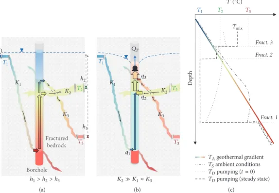
3.2. Conceptual Example of Temperature Profiles in a Fractured Aquifer. Figure 2 aims to conceptually describe a scenario
whereby the hydrogeological context, the bedrock fracture network, and the presence of a well (pumped or not) will drive advection and conduction heat fluxes induced by flowing water. These heat fluxes will modify the temperature field within the system, which could be revealed and described through the measurement of temperatures within the bore-hole. To simplify, the background geothermal gradient in Figure 2 is considered to be linear; that is, it does not represent a realistic gradient, which is usually multicurved in the upper part, because of seasonal and climatic atmospheric tempera-ture variations [19]. The bedrock aquifer in Figure 2 has three distinct fractures, not connected with one another except at the location of the borehole. These fractures have different
inclinations, hydraulic conductivities (𝐾2 ≫ 𝐾1 ≈ 𝐾3),
original temperatures (according to the linear geothermal
gradient𝑇3 > 𝑇2 > 𝑇1), and hydraulic heads (ℎ1 > ℎ2 > ℎ3)
at their furthest extents from the borehole. In this example, heads arbitrarily decrease with depth.
The situation under ambient conditions is presented in Figure 2(a). The highest hydraulic head at the outermost extent of fracture 1 induces an ambient flow that is redis-tributed between fractures 2 and 3. The flow distribution between the fractures is controlled by the hydraulic poten-tial, which combines the hydraulic transmissivity and the hydraulic gradient between the fractures. In this example,
even if𝐾2 > 𝐾3, it is possible that fracture 3 drains a larger
proportion of the ambient flow. This can occur if the head gradient between fracture 1 and fracture 3 is high enough that the hydraulic potential is higher than that between fracture 1 and fracture 2. This ambient flow induces a specific
temperature profile (𝑇𝑆) in the wellbore (Figure 2(c)). 𝑇𝑖
from fracture 1 is slightly colder than𝑇𝐴, because the heat
advection due to ambient flow along the fracture 1 network is strong enough to avoid its complete reequilibration with
𝑇𝐴. The water flowing upwards then exchanges heat with
the borehole walls by heat conduction, implying that the
𝑇𝑆 profile differs from the𝑇𝐴profile. At fracture 2, part of
the flow is drained out, so that the total flow within the borehole is reduced, inducing a relatively greater potential for temperature reequilibration by conduction with the borehole
wall (increasing the slope of the𝑇𝑆profile between fracture 2
and fracture 3). Up to fracture 3,𝑇𝑆is the same as𝑇𝐴, since
no ambient flow influences its profile.
The situation under pumping conditions is presented in Figure 2(b). Due to the pumping, water drawdown into the well imposes the drainage of all active fractures into the wellbore, proportionally to the transmissivity of each fracture. As the pump is placed at the top of the well, flow in the borehole is unidirectional and gradually increases from the lowest to the highest active fracture. Flow intensities during pumping depend on hydraulic properties. However, compared to ambient conditions, flow intensities would be much higher during pumping because active fractures are more strongly solicited and the advection heat flux will become greater than the conduction heat flux. Consequently, the temperature of each inflow discharging into the borehole would be much closer to the temperature of the groundwater
Fractured bedrock Borehole ℎ1 ℎ2 ℎ3 K1 K2 K3 T1 T2 T3 ℎ1> ℎ2> ℎ3 (a) K1 K2 K3 T1 T2 T3 K2≫ K1≈ K3 QT q3 q2 q1 (b) De p th Fract. 3 Fract. 2 Fract. 1 T1 T2 T3 TAgeothermal gradient TSambient conditions TDpumping (t ≈ 0) TDpumping (steady state)
TGix T (∘C)
(c)
Figure 2: Conceptual schematic of temperature profiles in a fractured aquifer: (a) ambient scenario, (b) pumping scenario, and (c)𝑇𝑆and 𝑇𝐷temperature profiles in the borehole.
at the far end origin of its fracture network.𝑇𝑖at fracture 1
becomes colder under pumping conditions, because advec-tion dominates over conducadvec-tion. Once inside the borehole, upward flowing water from fracture 1 would still be subject to conduction-driven reequilibration with the temperature of the borehole wall. However, as its flow rate is much greater during pumping, the relative conductive heat flux is much lower than under ambient conditions. For the short pumping
duration (𝑡 ≈ 0) in Figure 2(c), the 𝑇𝐷 profile can still
slightly reequilibrate with𝑇𝑆, but as advection will quickly
dominate during pumping, the𝑇𝐷profile is less influenced
by conductive reequilibration with the borehole wall. 𝑇𝐷
between fractures 2 and 3 is determined by the advective mixing of inflow from fractures 1 and 2 (flow rates and
𝑇𝑖) at the beginning of pumping. With increasing pumping
duration, a thermal steady state would eventually be reached
(Figure 2(c)). Every𝑇𝑖will be influenced by the orientation
of the fracture system. If the fracture network is inclined, thermal reequilibration within the aquifer could occur, so
𝑇𝑖 would range between 𝑇𝐴 (at the far end of the fracture
network) and𝑇𝐴(where the facture intercepts the borehole).
𝑇𝑖resulting from very inclined fractures and high flows would
be closer to the temperature at the far end of the drainage system. Conversely, if the fracture network is horizontal and
flow is weak,𝑇𝑖 would be nearly equal to the temperature
imposed by the background geothermal gradient,𝑇𝐴, at the
given depth. When advection controls over conduction (i.e.,
at steady state in Figure 2(c)):𝑇𝑖fracture 2 ≈ 𝑇2,𝑇𝑖fracture 1 ⪆
𝑇1, and𝑇𝑖fracture 3 ⪅ 𝑇3. The temperature of the total flow
discharged at the wellhead (𝑇mixin Figure 2(c)) would mainly
be determined by the mixing of inflows from fractures 1, 2, and 3, in proportion to their respective inflow intensities and temperatures.
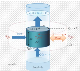
3.3. Heat Budget at the Borehole Scale. The heat budget at the
scale of a given volume (𝑑𝑉) of the borehole is presented
in Figure 3. 𝑑𝑉 is defined by the interval separating two
passive temperature measurements,𝑇(𝑧 + 1) and 𝑇(𝑧 − 1).
During pumping, water mixing occurs between groundwater
inflow, 𝑞(𝑧) (being positive if water enters the borehole
and negative if water flows outward) at temperature𝑇𝑖(𝑧),
and water flowing upward (𝑄(𝑧 − 1)) in the borehole at
temperature 𝑇𝐷(𝑧 − 1). The heat budget of mixing these
volumes corresponds to the difference in heat transported by
the volume of water entering the base(𝑄(𝑧 − 1)) and flowing
though the wall between𝑧 − 1 and 𝑧 + 1 (inflow 𝑞(𝑧)) and
that transported by the water leaving𝑑𝑉 at 𝑧 + 1 (𝑞(𝑧) + 𝑄(𝑧
−1)).
For a quantity of water that is either heated or cooled, the
general expression of advection heat flux,𝜙adv(W), is given by
(2) [41], where𝑄 (m3/s) is the water flow rate,𝐶 (J m−3∘K−1)
is the specific volumetric thermal capacity of water, and𝑇𝑖
and 𝑇𝑓 are the initial and final temperatures of the water,
respectively.
Borehole Aquifer q(z) + Q (z − 1) TD(z + 1) dz dV TD(z − 1) Q (z − 1) TS(z + 1) Td(z) Ti(z) Ts(z) TS(z − 1) ri re q(z) =IH>
Figure 3: Heat budget at the borehole scale.
Considering (2) and the adiabatic mixing of two fluids at
different temperatures, the heat balance of water fluxes𝑞(𝑧)
and𝑄(𝑧 − 1) that mix in the borehole is given by
𝑞 (𝑧) 𝐶 [𝑇𝐷(𝑧) − 𝑇𝑖(𝑧)]
+ 𝑄 (𝑧 − 1) 𝐶 [𝑇𝐷(𝑧 + 1) − 𝑇𝐷(𝑧 − 1)] = 0.
(3) Once pumping is initiated, the borehole wall temperature
quickly shifts from𝑇𝑆 to𝑇𝐷. Heat conduction then occurs
radially through the surface of the borehole. The general expression of radial conductive heat transfer at steady state through a semi-infinite solid [41] is applied. In this case, the finite boundary is the borehole wall, which is subject to a temperature shift due to pumping. The temperature anomaly will propagate within the semi-infinite solid (e.g., the aquifer). Heat conduction flux between the borehole wall
and the aquifer is then given by (4), where𝑑𝑧 is the length
of the interval,𝑇𝑠(𝑧) and 𝑇𝐷(𝑧) are the mean temperatures
of the water in the borehole under static conditions and
during pumping respectively, averaged for the interval 𝑑𝑧,
𝑟𝑖(m) is the radius of the well,𝑟𝑒(m) is the time-dependant
radius of the heat conduction influence around the borehole,
and 𝑥 = 𝑟𝑒 − 𝑟𝑖 is the annular distance of propagation
of the temperature anomaly due to pumping (𝑇𝐷 − 𝑇𝑆),
which dissipates into the aquifer. With increasing pumping
duration,𝑟𝑒increases in (5), so that the heat conduction flux
fades during pumping. 𝜆 (W m−1∘K−1) is the bulk thermal
conductivity of the aquifer.
𝜙cond=
2𝜋𝜆𝑑𝑧 [𝑇𝑆(𝑧) − 𝑇𝐷(𝑧)]
ln(𝑟𝑒/𝑟𝑖) . (4)
Considering advection and conduction heat fluxes, the heat balance at the borehole scale is given by (5), which combines (3) and (4): 𝑞 (𝑧) 𝐶 [𝑇𝐷(𝑧) − 𝑇𝑖(𝑧)] + 𝑄 (𝑧 − 1) 𝐶 [𝑇𝐷(𝑧 + 1) − 𝑇𝐷(𝑧 − 1)] = 2𝜋𝜆𝑑𝑧 [𝑇𝑆(𝑧) − 𝑇𝐷(𝑧)] ln(𝑟𝑒/𝑟𝑖) . (5) This equation then links the measured temperature-depth
profiles (i.e., 𝑇𝑆(𝑧) and 𝑇𝐷(𝑧)) with three variables: 𝑞(𝑧),
𝑇𝑖(𝑧), and 𝑟𝑒 (which increases with pumping duration).
𝑞(𝑧) distribution could also be measured independently, for example, with a flowmeter.
4. Results
4.1. Depth-Temperature Profiles Modelled with the Heat Bud-get. In this section, temperature-depth profiles were
mod-elled for dynamic conditions (𝑇𝐷(𝑧)), considering a
concep-tual well which intercepts six hydraulically active fractures (Figure 4). In this example, the percentage of total pumping
discharge (%𝑄𝑇(𝑧)) and temperature (𝑇𝑖(𝑧)) associated with
each inflow have been randomly and arbitrarily set with depth. In order to simplify the thermal static conditions, a linear geothermal gradient was applied (arbitrarily set to
−1∘C/100 m), with an absence of ambient flows so that𝑇𝑆(𝑧) =
𝑇𝐴(𝑧). Pumping occurs at the top of the wellbore, inducing
upward water flows. Blue arrows in Figures 4(b) and 4(c) represent water flow directions in the water column and
inflow from the aquifer. The𝑇𝐷(𝑧) response to pumping was
modelled using the heat budget (see (5)) implemented in
a spreadsheet, with a vertical resolution𝑑𝑉 = 0.5 m. Fixed
parameters used for the model are as follows: radius of the
well,𝑟𝑖 = 0.075 m, bulk thermal conductivity of the aquifer,
𝜆, = 𝜆𝑠(1−𝑛)𝜆𝑤𝑛 = 1.88 W m−1∘K−1, effective porosity, 𝑛, =
0.05, and thermal conductivity of sedimentary bedrock,𝜆𝑠,
= 2.0 Wm−1∘K−1 and of water, 𝜆𝑤, = 0.6 W m−1∘K−1 [42].
Various conditions for heat advection and conduction fluxes were simulated to evaluate their effect on the shapes of the
𝑇𝐷(𝑧) profiles. The effect of heat advection (at the given heat
conduction,𝑟𝑒, = 0.091 m) was investigated by varying the
total pumping rate from 𝑄𝑇 = 1 L/min to𝑄𝑇 = 100 L/min
(Figure 4(b)), and the effect of heat conduction (at the given
heat advection,𝑄𝑇, = 40 L/min) was investigated by varying
𝑟𝑒from 0.076 to 0.101 m (Figure 4(c)). In both simulations,
𝑇𝐷(𝑧) profiles are also provided by considering only heat
advection. Conduction is neglected by setting𝜙cond = 0 in
(5). This is theoretical, because in reality conduction always
occurs, but the latter 𝑇𝐷(𝑧)𝜙cond = 0 profiles are helpful
to Figure 4 for visually distinguishing when heat advection becomes dominant over heat conduction.
4.1.1. General Patterns and Processes Controlling Modelled Depth-Temperature Profiles. The positions of water inflows
into the wellbore are easily identifiable in the dynamic
temperature profiles in Figure 4. However, even if𝑞 (5 m)
= 20%𝑄𝑇and𝑞 (20 m) = 10% 𝑄𝑇(Figures 4(b) and 4(c)),
the occurrence of these large inflows is not very well-revealed
from the𝑇𝐷profile, because𝑇𝑖(5 m)≈ 𝑇𝐷(5 m) and𝑇𝑖(20 m)
50 45 40 35 30 25 20 15 10 5 0 D ep th (m) 0 25 50 75 100 % QT (a) 50 45 40 35 30 25 20 15 10 5 0 D ep th (m) 20% QT 50% QT 10% QT 13% QT 5% QT 2% QT re= 0,09 G Ts (static) Ti (GW inflow) TD QT = 1 ,/GCH TD QT = 2 ,/GCH TD QT = 5 ,/GCH TD QT = 20 ,/GCH TD =IH> = 0 9,0 9,1 9,2 9,3 9,4 9,5 9,6 T (∘C) (b) 50 45 40 35 30 25 20 15 10 5 0 D ep th (m) QT= 5 ,/GCH 9,0 9,1 9,2 9,3 9,4 9,5 9,6 T (∘C) Ts (static) Ti (GW inflow) TD =IH> = 0 TD Re = 0,076 G TD Re = 0,08 G TD Re = 0,09 G TD Re = 0,1 G TD Re = 0,2 G 20% QT 50% QT 10% QT 13% QT 5% QT 2% QT (c) Figure 4: Dynamic depth-temperature profiles modelled with the heat budget.
pumping conditions favor heat conduction (i.e., lower total
discharge in Figure 4(b) or lower𝑟𝑒values in Figure 4(c)).
As𝑇𝐷profiles are derived from both advection and
con-duction heat fluxes, the shape of the temperature profiles does not directly (graphically) reflect the water flow distribution in the wellbore. In Figures 4(b) and 4(c), temperature profiles do not mimic the shape of water flow distribution in the
wellbore. Even when conduction is neglected (𝑇𝐷𝜙cond. = 0
in Figures 4(b) and 4(c)), the resulting𝑇𝐷 profiles still do
not directly reflect water flow distribution in the wellbore. Another important characteristic to note is that when
con-duction is (or becomes) negligible in this case,𝑇𝐷(𝑧) profiles
are entirely controlled by the distribution of inflows into the wellbore, independently of the total discharge rate.
𝑇𝐷 profiles appear to be extremely sensitive to very
low groundwater inflows into the wellbore, especially at the bottom intervals for this example, where the total flow of
water remains low. In this example, the bottom inflow, 𝑞
(45 m), would be detectable for flows as low as 0.02 L/min
(e.g., in Figure 4(b), where𝑞 (45 m) = 2% of 𝑄𝑇= 1 L/min,
with medium conduction,𝑟𝑒= 0.091 m) or as low as 0.1 L/min
(e.g., in Figure 4(c), where𝑞 (45 m) = 2% of 𝑄𝑇= 5 L/min,
with intense conduction,𝑟𝑒= 0.076 m).
As 𝑇𝐷(𝑧) profiles depend on the temperature of each
inflow, the range for each𝑇𝑖(𝑧) could be qualitatively
esti-mated by visualizing the cooling (e.g.,𝑇𝑖(𝑧) < 𝑇𝐷(𝑧)) or
warming (e.g., 𝑇𝑖(𝑧) > 𝑇𝐷(𝑧)) of the water column where
steps in the profile occur.
The influence of heat conduction fluxes could become less important than heat advection with increasing pumping time and/or with increasing water flow rates in the borehole.
In Figure 4(b) (representing increasing pumping rates),𝑇𝐷
profiles become dominated by heat advection for𝑄𝑇(35 m)>
1.4 L/min (e.g., 7% of𝑄𝑇= 20 L/min at depths shallower than
35 m). In Figure 4(c) (representing increasing pumping time;
e.g., increasing𝑟𝑒, with𝑄𝑇 = 5 L/min),𝑇𝐷 profiles become
dominated by heat advection as soon as𝑟𝑒 > 0.081 m for
𝑄𝑇(35 m)> 0.35 L/min (e.g., 7% of 𝑄𝑇= 5 L/min at depths
shallower than 35 m). It is important to note that a radius of
influence of𝑟𝑒= 0.081 m represents a temperature front due to
pumping that radially penetrates only 6 mm into the aquifer
(𝑟𝑖= 0.075 m in this case).
Another way to look at the respective influences of advection and conduction fluxes at the borehole scale is given in Figure 5, which provides a comparison of advection and conduction fluxes calculated at the borehole scale using (2) and (4). Advection heat flux in the wellbore is related to flow and to the cooling or warming of the water (Δ𝑇) due to inflowing groundwater. Conduction heat flux between
the borehole wall (at 𝑇𝐷) and the aquifer (at 𝑇𝑆 = 𝑇𝐴)
varies logarithmically with the propagation distance (𝑥 =
50 100 150 200 250 300 350 400 0 Heat flux (W) 0 1 2 3 4 5 6 7 8 9 10 Flo w in t h e b o reho le (L/min)
advection intensity (water flow and temperature) ΔT (temperature offset of the water due to water
inflow into the borehole)
0.1∘
C 0.2∘C
0.3∘
C 0.4∘C
0.5∘C
conduction intensity (borehole wall/aquifer) (borehole interval: 1 m, effective porosity: 0.05)
ΔT (initial temperature offset TD− TSat the beginning of the pumping)
0.1∘C 0.2∘C 0.3∘C 0.4∘C 0.5∘C 0 1 2 3 4 5 6 7 8 9 10 11 12 13 14 15 Dist an ce t o b o reho le wall x= re −r i (cm)
Figure 5: Comparison of advection and conduction heat fluxes at the borehole scale.Φadvection=𝑓 (total flow rate, temperature offset due to groundwater inflow) andΦconduction=𝑓 (distance of radial
temperature propagation into the aquifer,𝑇𝐷− 𝑇𝑆offset).
Conduction flux is therefore intense at the beginning of the
pumping (𝑟𝑒 ≈ 𝑟𝑖) and fades with pumping duration (i.e.,
with increasing𝑟𝑒). Interpretation of Figure 5 indicates that
conduction flux is higher than advection flux when flow rates are less than 1 L/min and when temperature propagation is
less than approximately 1.5 cm into the aquifer (𝑟𝑒 = 0.09 m;
𝑟𝑖= 0.075 m). Conversely, if water flow is greater than 1 L/min
in the borehole, with increasing pumping duration (i.e.,𝑥 >
1.5 cm), advection fluxes become higher than conduction.
4.1.2. Potential of a High-Resolution Temperature Probe to Be Used as a Flowmeter. A relevant question is whether
passive temperature measurements could directly reflect the water flow distribution in the wellbore. This question is investigated in this section by modelling depth-temperature
dynamic profiles with the heat budget, with𝑇𝑖(𝑧), 𝑞𝑖(𝑧), and
𝑟𝑒 as variables. The fitting procedure consists of minimizing
the root mean square error (RMSE) of𝑇𝐷 (see (6)), where
𝑇𝐷reference(𝑧) represents the observed temperature-depth
pro-files,𝑇𝐷model(𝑧) represents the modelled temperature-depth
profiles,𝐷totalis the total depth of the wellbore, and𝑑𝑧 is the
vertical resolution of the heat budget.𝐷total/𝑑𝑧 represents the
number of𝑇𝐷model(𝑧) calculated with the heat budget.
RMSE𝑇𝐷= √∑ (𝑇𝐷model(𝑧) − 𝑇𝐷reference(𝑧))
2
𝐷total/𝑑𝑧
. (6)
In this example, the fitting procedure has 13 variables (6𝑇𝑖(𝑧),
6𝑞𝑖(𝑧), and 𝑟𝑒) and is constrained by 100𝑇𝐷(𝑧) observations
(well depth of 50 m, with a vertical resolution of𝑑𝑧 = 0.5 m).
To avoid divergence of the iterative procedure,𝑇𝑖(𝑧) variables
were initialized and constrained for each water inflow. Inflow
8,7 8,8 8,9 9,0 9,1 9,2 9,3 9,4 9,5 9,6 9,7 9,8 9,9 T (∘C) 50 45 40 35 30 25 20 15 10 5 0 TS TD reference Ti initial Ti range re= 0,10 G QT= 1 ,/GCH
Figure 6: Example of𝑇𝑖(𝑧) initialization prior to 𝑇𝐷(𝑧) modelling with the heat budget.
temperatures 𝑇𝑖(𝑧) were initialized at 𝑇𝐷reference(𝑧) (𝑇initial
in Figure 6) and constrained within the range of𝑇𝑖(𝑧) =
𝑇𝐷reference(𝑧) ± Δ𝑇 (𝑇𝑖range in Figure 6). The temperature range is logically anchored depending on the cooling or
warming of the 𝑇𝐷 profile resulting from inflows. For the
situation wherein the water column is cooling (because
of cold inflow), the range is set to 𝑇𝐷reference(𝑧)–Δ 𝑇 <
𝑇𝑖range < 𝑇𝐷reference(𝑧) and vice versa for a warming situation (𝑇𝐷reference(𝑧) < 𝑇𝑖range< 𝑇𝐷reference(𝑧) + Δ𝑇). In this example,
Δ𝑇 was arbitrarily set to 0.4∘C, but a large possible range over
which𝑇𝑖(𝑧) may vary is permitted before the fitting procedure
converges. Water inflow intensities were all initialized at very
low flows (𝑞𝑖(𝑧) = 0.0001 L/min) and constrained so that the
total modelled discharge must be equal to the total reference discharge. Finally, conduction in the borehole is initialized
as being intense (𝑟𝑒 = 0.076 m) and constrained within the
possible range (i.e.,𝑟𝑒> 𝑟𝑖).
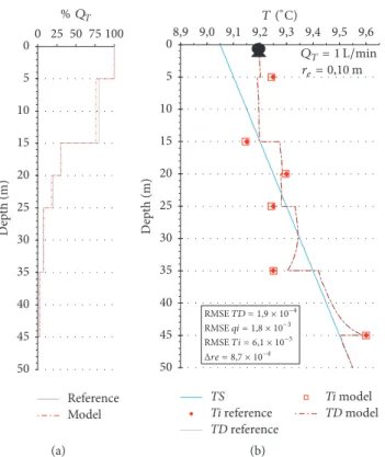
For modelling, two reference 𝑇𝐷reference profiles were
generated using the conceptual model (as described at the
beginning of Section 4.1), with conduction set to𝑟𝑒= 0.10 m
and total pumping rates of 1 L/min (Figure 7) and 20 L/min (Figure 8).
The fitting procedure very efficiently models 𝑇𝐷(𝑧) in
both cases. As shown in Figures 7 and 8,𝑇𝐷referenceand𝑇𝐷model
appear graphically superimposed. Numerically, some dis-crepancies remain, but the RMSE remains low in both cases
(RMSE𝑇𝐷 ≈ 10−4). The fitting procedure adequately models
the whole system at a low discharge rate (𝑄𝑇 = 1 L/min,
Figure 7), associated with low error for each variable;𝑇𝑖(𝑧)
(RMSE𝑇𝑖= 1.2× 10⁻⁵∘C),𝑞𝑖(𝑧) (RMSE 𝑞𝑖= 1.8× 10⁻³L/min),
0 25 50 75 100 % QT 50 45 40 35 30 25 20 15 10 5 0 D ep th (m) Reference Model (a) 8,9 9,0 9,1 9,2 9,3 9,4 9,5 9,6 T (∘C) 50 45 40 35 30 25 20 15 10 5 0 D ep th (m) TS Ti reference TD reference Ti model TD model re= 0,10 G QT= 1 ,/GCH RMSE TD = 1,9 × 10⁻⁴ RMSE qi = 1,8 × 10⁻³ RMSE Ti = 6,1 × 10⁻⁵ Δre = 8,7 × 10⁻⁴ (b)
Figure 7: Results of𝑇𝐷(𝑧) modelling with the heat budget at 𝑄𝑇= 1 L/min. (a) Flow-depth distribution; (b) dynamic temperature profiles (𝑇𝐷(𝑧)) and temperatures of inflows (𝑇𝑖(𝑧)).
50 45 40 35 30 25 20 15 10 5 0 De pth ( m ) Reference Model 0 25 50 75 100 % QT (a) TS Ti reference TD reference Ti model TD model 50 45 40 35 30 25 20 15 10 5 0 De pth ( m ) re= 0,10 G QT= 20 ,/GCH 8,9 9,0 9,1 9,2 9,3 9,4 9,5 9,6 T (∘C) RMSE TD = 1,7 × 10⁻⁴ RMSE qi = 180 RMSE Ti = 1,2 × 10⁻² Δre = 1,7 × 10⁻² (b)
Figure 8: Results of𝑇𝐷(𝑧) modelling with the heat budget at 𝑄𝑇= 20 L/min. (a) Flow-depth distribution; (b) dynamic temperature profiles (𝑇𝐷(𝑧)) and temperatures of inflows (𝑇𝑖(𝑧)).
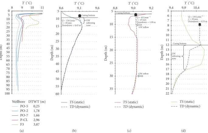
0,25 2,96 1,66 1,78 3,87 Wellbore DTWT (m) PO-5 P-CL PO-7 PO-2 F3 100 95 90 85 80 75 70 65 60 55 50 45 40 35 30 25 20 15 10 5 0 D ep th (m) 8 9 10 11 T (∘C) (a) TS (static) TD (dynamic) Casing bottom GW inflowing zone 60 55 50 45 40 35 30 25 20 15 10 5 D ep th (m) 8,6 9,1 9,6 T (∘C) Q = 150 ,GCH−1 t = 19 GCH $L;Q>IQH = 0,45 G (b) TS (static) TD (dynamic) Casing bottom GW inflow GW inflow 35 30 25 20 15 10 5 D ep th (m) 8,8 9,0 9,2 T (∘C) Q = 45 ,GCH−1 t = 43 GCH $L;Q>IQH = 1,90 G (c) Casing bottom GW inflowing zone TS (static) TD (dynamic) 22 21 20 19 18 17 16 15 14 13 12 11 10 9 8 7 6 5 D ep th (m) 9,4 9,9 10,4 T (∘C) Q = 150 ,GCH−1 t = 29 GCH $L;Q>IQH = 0,53 G (d)
Figure 9: Temperature profiles in June 2016 for all wells under static conditions (a) and under static and dynamic conditions for wells PO-7 (b), P-Cl (c), and F3 (d).
discharge rate (𝑄𝑇= 20 L/min, Figure 8), errors for modelled
variables increase, with RMSE𝑇𝑖= 1.2× 10⁻²∘C, RMSE𝑞𝑖=
180 L/min, andΔ𝑟𝑒= 1.7× 10⁻²m. The ability of the model to
converge to accurate variable values depends on the degree
of curving for the 𝑇𝐷(𝑧) profiles. The more the profile is
curved along the entire profile due to the dominant influence of conduction over advection, the easier the fitting procedure can converge within a narrow, accurate range for the variables
𝑇𝑖,𝑞𝑖, and 𝑟𝑒. Even a very slight influence of conduction would
theoretically induce a slight curvature in𝑇𝐷(𝑧), so that the
model can theoretically always be solved. However, with the diminishing influence of conduction, the preciseness (and complexity) of the fitting procedure has to proportionally increase to still obtain the narrowest and most accurate range of solutions for the variables. At the other extreme, if there is no conduction at all, the model can still perfectly converge to
fit the𝑇𝐷(𝑧) profiles, but an infinity of solutions is possible for
each pair of𝑇𝑖(𝑧) and 𝑞𝑖(𝑧) associated with the inflows. This is
because, without conduction, any variation in𝑇𝑖(𝑧) could be
numerically compensated by𝑞(𝑧) to give the same perfectly
square𝑇𝐷(𝑧) profiles that are observed after mixing.
4.2. Field Applications
4.2.1. Qualitative Interpretation of Field Depth-Temperature Profiles. PO-2, PO-5, and PO-7 temperature logs under static
conditions (Figure 9(a)) were taken on the same day and represent typical static temperature profiles not influenced
by ambient flows. Heat pulse flowmeter tests [43] were performed for well PO-7 under static conditions and did not allow the detection of water circulation in the borehole (the minimum velocity resolution of the device is 0.113 L/min). As PO-2, PO-5, and PO-7 temperature profiles have the same symmetrical curving, it is inferred that ambient flows are so low, if there are any at all, that they do not significantly impact the temperature profiles of these three wells. The
correspond-ingTS profiles of the three wells differ by 0.1–0.5∘C, which
may be explained by different local recharge rates, the nature and thickness of the unconsolidated sediments, or differences in land cover. These discrepancies are not considered further in this work, which focuses rather on borehole logging to
characterize active hydraulic fractures.Ts profiles for wells
PO-2, PO-5, and PO-7 are therefore considered to be
repre-sentative of typicalTAprofiles of southern Quebec: (1) the
seasonal variation in soil temperature (from the atmospheric signal) propagates from the land surface down to 15 m depth. The minimum temperature, near 5 m depth, corresponds to the cold temperature signal of winter 2015-2016, which has propagated into the subsurface; (2) from 15 m to 50–60 m, temperatures decrease with depth. This inverse gradient can be explained by the climatic warming in Canada over the last 150–200 years [44]; and (3) deeper than 50–60 m, which corresponds to the transition zone to the normal geothermal gradient, temperatures increase with depth.
Static and dynamic temperature logs of the three pumped wells are superimposed in Figure 9. The PO-7 temperature
log under dynamic conditions (Figure 9(b)) was taken after 19 min of pumping with a discharge rate of 150 L/min. Static and dynamic temperature profiles differ near the surface, down to 13 m depth, and are nearly identical below this depth
(i.e.,𝑇𝑆 = 𝑇𝐷). This indicates that the productivity of this
52 m screened well essentially originates from an only 4 m-long productive interval in the upper part of the well.
For well P-Cl, the static temperature log (Figure 9(a)) already suggests the presence of ambient flow between 15 and 30 m, because the constant temperature within this
interval differs from the expected curved𝑇𝐴profile. Although
the direction and intensity of ambient flows could not be
determined at this stage, the𝑇𝑆profile already reveals that
an ambient flow of water at 9.04∘C is circulating between
one or more fractured intervals located in the 15–30 m depth
range. The P-Cl dynamic 𝑇𝐷 profile, taken after 40 min of
pumping with a discharge rate of 45 L/min, confirms the
information revealed by the𝑇𝑆profile but also indicates that
the main productive zone must be located near 30 m depth,
because its inflow temperature (9.04∘C) completely resets the
temperature of the water circulating upward along the entire length of the borehole. Other small water inflows from 10 m to 30 m depth may be possible, but as no temperature variation is distinguishable in this interval, the main inflow must be located at approximately 30 m depth.
The𝑇𝑆profile for well F3 (Figure 9(d)) also suggests the
presence of ambient flows, because between 12 and 17 m the profile is overcurved compared to what would be expected
from the influence of𝑇𝐴alone. This suggests that more than
two active fracture zones are likely located within the interval between 12 and 17 m, thus creating a complicated temperature pattern. Ambient flows between these active fractures create
this anomalous temperature interval. In F3, the 𝑇𝐷 profile
(Figure 9(d)) was taken after 29 min of pumping with a
discharge rate of 150 L/min. As 𝑇𝑆 and 𝑇𝐷 coincide below
17 m, no active fracture is expected to be present below this depth. Joint analysis of passive and dynamic logs qualitatively reveals the following: (1) the first active fracture zone is located between 16 and 17 m depth and initiates water flow into the borehole, with a bottom inflow temperature of
10.00∘C; (2) between 16 and 13 m depth, one single qualitative
interpretation is not possible. The temperature gradient retains the same orientation and intensity between each measurement. This could either indicate that warmer water
is inflowing (𝑇𝑖 > 𝑇𝐷) or that temperature reequilibration
by conduction occurs between the borehole and a warmer
aquifer neighboring the borehole (𝑇𝑆> 𝑇𝐷) or a combination
of these two scenarios. And, finally, (3) between 12 and 13 m, the slope of the dynamic log increases strongly, which can
only be explained by warmer water inflow (𝑇𝑖 > 𝑇𝐷), which
increases substantially.
4.2.2. Quantitative Borehole Investigation: Temperature Log-ging, Flow Metering, and Televiewing. Flowmeter logging in
boreholes PO-7 and F3 was performed with pumping rates as high as possible, depending on the productivity of the given well, in order to maximize water velocities in the boreholes. Different pumping rates were tested on each of the wells (results not shown in this article), with no measurable
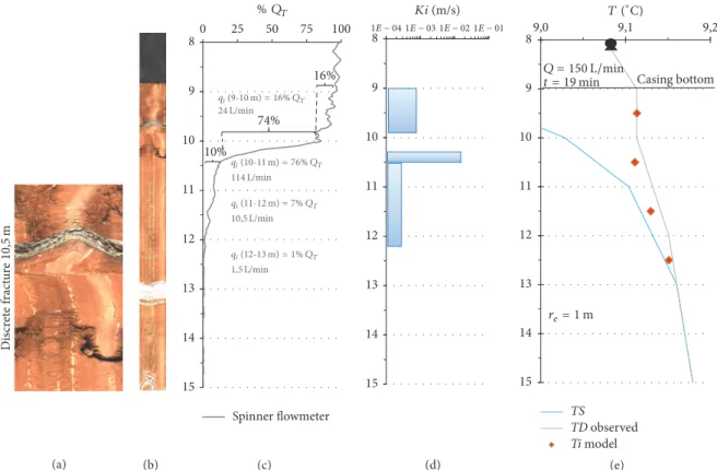
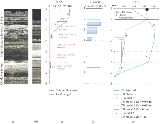
variation in well inflow distribution found to result with depth. The PO-7 televiewing results are presented in Figures 10(a) and 10(b), and the flowmeter log is presented in Fig-ure 10(c). The flowmeter log revealed that 10% of total inflows originate from a low-fractured interval, located between 12 and 13 m. A discrete fracture is visible at 10.5 m and alone accounts for 74% of the total productivity of the well. The remaining 16% of the inflow originates from a joint or fracture located at 9.6 m depth and from other small fractures located above this and down to the base of the casing. For well F3 (televiewing in Figures 11(a) and 11(b); flowmeter log in Figure 11(c)), small conduits are identifiable through televiewing at 16.5 m depth. Flowmeter measurements show that these conduits account for approximately 7% of the total well productivity. No other water inflow is identifi-able through the flowmeter results until above 14 m depth. Televiewing also revealed information about the thickness of strongly fractured banks that alternate with unfractured dolomite intervals. Based on flowmeter results where flow increases, fractured zones from 14 to 13.7 m, 13.4 to 12.8 m, and 12.6 to 12.3 m account for approximately 3, 31, and 46% of the total transmissivity of well F3, respectively. The remaining 13% of the transmissivity likely originates from fractures located near the base of the casing. For wells PO-7 and F3, the distribution of hydraulic conductivities for each productive fractured interval are given in Figures 10(d) and 11(d), respectively, and have been calculated using (1). It should be noted that the spinner flowmeter provided highly valuable hydrogeological information here, with a high vertical resolution (5 cm in this work), and was obtained relatively quickly (i.e., less than half an hour to log a 60 m deep well).
Temperature logs under static and dynamic conditions are presented in Figures 10(e) and 11(e) for wells PO-7 and F3, with close-ups of depth intervals where water inflow
occurs and influences 𝑇𝐷(𝑧) profiles. The full-depth scale
temperature logs are presented in Figure 9. The heat budget (see (5)) was partially used in this applied case, because the measurement resolution (𝑑𝑧 = 1 m) for the available data is insufficient to perform the full fitting procedure presented in Section 4.1.2. Also, at the time of measurement, high discharge rates were set to maximize the sensitivity of the flowmeter, while the thermal fitting procedure would instead require low discharge rates to favor conduction (Section 4.1.2). Nevertheless, the heat budget was applied for wellbore PO-7, to calculate mean inflow temperatures (Fig-ure 10(e)), with flow distribution intervals known from flow metering. Given high flow rates and pumping times,
conduc-tion was set to low intensity (𝑟𝑒= 1 m). For PO-7, calculated
𝑇𝑖(𝑧) were all warmer than 𝑇𝑆(𝑧) at a 13 m depth, indicating
that pumping-induced drainage might all originate from very
surficial and warmer horizons, above 5 m depth (𝑇𝑆(𝑧) profile
in Figure 9(a)), influenced by the previous summer’s signal
propagation within the subsurface. For well F3,𝑇𝑖(𝑧) can be
calculated for very high inflow intervals (12 to 13 m, 13 to
14 m, and 16 to 17 m), with respective𝑞𝑖(𝑧) measured with the
flowmeter (model 1 in Figure 11(e)). For two other intervals (14 to 15 m and 15 to 16 m), flow metering did not reveal any increase in flow, resulting in the nondetection of inflows
Dis cr et e f rac tur e 10,5 m (a) (b) Spinner flowmeter 74% 10% 16% 15 14 13 12 11 10 9 80 25 50 75 100 % QT qi(9-10 m) = 16% QT 24 L/min qi(10-11 m) = 76% QT 114 L/min qi(11-12 m) = 7% QT 10,5 L/min qi(12-13 m) = 1% QT 1,5 L/min (c) 15 14 13 12 11 10 9 8 1E − 04 1E − 03 1E − 02 1E − 01 Ki (m/s) (d) TS TD observed Ti model Casing bottom 15 14 13 12 11 10 9 89,0 9,1 9,2 T (∘C) Q = 150 ,/GCH t = 19 GCH re= 1 G (e)
Figure 10: Borehole PO-7 logging results: (a) televiewing close-up of the most productive fracture, (b) televiewing log, (c) flow distribution obtained by flowmeter, (d) vertical distribution of hydraulic conductivities obtained by flowmeter, and (e) temperature profiles under static and dynamic conditions and temperature of groundwater inflows calculated with the heat budget.
within these intervals. However, 𝑇𝐷(𝑧) profiles between 14
and 16 m show significant temperature increases. As total advection flow in the water column is already high above 16 m depth (10.5 L/min), increasing temperature between 16 and 14 m cannot be explained by conduction reequilibration
towards 𝑇𝑆(𝑧). Examples are given in Figure 11(e) (model
1), representing modelled 𝑇𝐷(𝑧) for various conduction
intensities, but with no inflows between 14 and 16 m depth.
In this case,𝑇𝐷(𝑧) modelled between 14 and 16 m could not
fit the observed𝑇𝐷(𝑧) at any conduction intensity without
introducing inflows at this interval. The heat budget fitting procedure was then applied to all intervals, including inflows to the 14 to 15 m and 15 to 16 m intervals (model 2 in
Figure 11(e)). Conduction intensity in the latter model(2) was
arbitrarily set to𝑟𝑒= 1 m, a value that lowers the influence of
conduction, given that the pumping time of the experiment
is 29 min. With model 2 (Figure 11(e)), warm inflows,𝑇𝑖
(14-15 m) = 10.70∘C and𝑇𝑖(16-17 m) = 10.51∘C, were estimated,
corresponding with𝑞 (14-15 m) = 0.69 L/min and 𝑞 (15-16 m)
= 0.75 L/min. These calculated values are not very accurate, because the fitting procedure is poorly constrained, with a
limited temperature observation (resolution of only 𝑑𝑧 =
1 m). In this case, warmer 𝑇𝑖(𝑧) could lead to even lower
𝑞𝑖(𝑧) while still perfectly fitting 𝑇𝐷(𝑧). Nevertheless, the
most relevant information here is that the combination of
temperature measurements (even at a resolution of 0.01∘C)
and heat budget analysis allows the occurrence of very low
inflows to be inferred among the much higher productive intervals characterizing wellbore F3. Discussion linking the
𝑇𝑖(𝑧) values of well F3 to the depth at which groundwater is
drained during pumping is provided in Section 4.2.3 through more detailed experiments and analysis.
4.2.3. Inference of Groundwater Origin from Transient Temper-ature Logging and Heat Budget Application. Two temperTemper-ature
logs were obtained for well F3, in June and November 2016.
In Figure 12(a),𝑇𝑠 measured in June 2016 showed a colder
water interval from 5 to 11 m depth (influenced by cold air temperature at the ground surface for winter 2015-2016), followed by a warmer zone from 11 to 17 m (influenced by warm air temperature at the ground surface for summer
2015).𝑇𝑠measured in November 2016 showed the influence
of summer 2016 from the top of the water table until 12 to 13 m depth and likely a smoothed downward propagation of the summer 2015 signal below 17 m. Figures 12(b) and 12(c)
present𝑇𝑠and𝑇𝐷for June and November 2016, respectively,
along with𝑇𝑖for each pumping time and discharge rate.𝑇𝑖
values were calculated using the heat budget at the borehole scale (see (5)) for the most productive intervals identified by flow metering (Section 4.2.2) to be 70, 23, and 7% of the total transmissivity of well F3 for the 12 to 13 m, 13 to 14 m, and 16 to 17 m depth intervals, respectively.
For both June and November logs, 𝑇𝑖 profiles already
H ig h ly f rac tur ed in ter val 12–14 m C o nd ui t a t 16,5 m (a) (b) Spinner flowmeter Heat budget 7% 3% 31% 46% 13% 18 17 16 15 14 13 12 110 25 50 75 100 % QT qi(12-13 m) = 70% QT qi(13-14 m) = 23% QT 105 L/min 34,5 L/min qi(14-15 m) = 0,46% QT 0,69 L/min qi(15-16 m) = 0,50% QT 0,75 L/min qi(16-17 m) = 7% QT 10,5 L/min (c) 18 17 16 15 14 13 12 111E − 04 1E − 03 1E − 02 Ki (m/s) (d) TS observed TD observed Ti model 1 TD model 1 Re = 0,076 m m TD model 1 Re = 0,078 m TD model 1 Re = 0,1 Ti model 2 m TD model 2 Re = 1 Casing bottom 18 17 16 15 14 13 12 119,9 10,1 10,3 10,5 10,7 T (∘C) t = 29 GCH Increasing re QT= 150 ,/GCH− (e)
Figure 11: Borehole F3 logging results: (a) televiewing close-up of productive intervals, (b) televiewing log, (c) flow distribution obtained by flowmeter and flow calculated with the heat budget between 14 and 16 m depth, (d) vertical distribution of hydraulic conductivities obtained by flowmeter, and (e) temperature profiles under static and dynamic conditions and temperature of groundwater inflows calculated with the heat budget.
discrepancies suggest that, soon after pumping began, 𝑇𝑖
patterns are influenced by inflows originating from active
fracture networks in equilibrium with𝑇𝐴. This also indicates
that ambient flows (between 12 and 17 m depth) imposing
the𝑇𝑆profiles around the borehole mask the𝑇𝐴profile.𝑇𝑖
temperatures then appear to be very rapidly controlled by the temperatures within drained horizons, the temperatures
of which depend on the seasonal 𝑇𝐴 signal. In June
(Fig-ure 12(b)),𝑇𝑖is warmest in the 12 to 13 m interval and must
drain the warmer horizon influenced by summer 2015 (13 to 16 m depth), because temperatures for over- and underlying
intervals are colder.𝑇𝑖for the two lower inflow intervals (13
to 14 and 16 to 17 m depth) are colder and, with respect to
the𝑇𝑆 profiles for June, could drain colder horizons either
above 11 m depth or below 17 m depth. However, analysis together with the November profiles (Figure 12(c)) shows that
𝑇𝑖from 13 to 14 and 16 to 17 m depth must drain cold water
originating from below 17 m, because intervals above 11 m depth are warmer and cannot explain such cold temperatures. Although the interpretation of temperature inflow patterns in Figures 12(b) and 12(c) remains difficult, one key piece
of information provided is that all𝑇𝑖 values become cooler
as pumping duration increases, independently of the season.
This suggests that cold water originates from horizons deeper than 17 m depth.
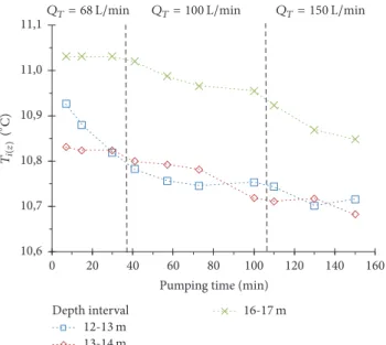
The evolution of inflow temperatures, 𝑇𝑖(𝑧), in well F3
during pumping in November is presented in Figure 13. The temperature range from the beginning to the end of pumping is comparable for every depth interval. This common cooling of all inflows with time suggests that all inflows drain strat-ified fractured horizons and have comparable orientations. It can be noted that, even after 150 min of pumping at high discharge rates (150 L/min at the final stage), none of the inflow temperatures reaches a plateau. This means that temperature equilibration by conduction between flowing groundwater and the aquifer has not yet reached a thermal steady state along the flow path from the origin of aquifer drainage to the wellbore. Even if it is not quantified here, this suggests rather long conduits or channelized flow paths. In such a case, the reequilibration of the water temperature by heat conduction would take longer, because surface exchange with the aquifer is low. Conversely, thermal conduction equilibration occurring in a highly homogeneously fractured aquifer (or even a porous medium) would reach a steady state much faster, as the water/aquifer surface exchange is much higher. Compared to the two other fractured intervals,
TS (June) TS (November) Casing bottom 9 10 11 12 13 T (∘C) 22 21 20 19 18 17 16 15 14 13 12 11 10 9 8 7 6 5 4 D ept h (m ) (a) TS (June) TD, 29 min min TD, 47 min TD, 65 min Ti, 29 min Ti, 47 min Ti, 65 9,5 10,0 10,5 T (∘C) 22 21 20 19 18 17 16 15 14 13 12 11 10 9 8 7 6 5 4 D ept h (m ) Q = 150 ,/GCH (b) Pumping time 10,5 11,0 T (∘C) 22 21 20 19 18 17 16 15 14 13 12 11 10 9 8 7 6 5 4 D ep th (m) Q = 150 ,/GCH Q = 100 ,/GCH Q = 68 ,/GCH TS (November) TD 68 LPM, 7 min TD 68 LPM, 15 min TD 68 LPM, 30 min TD 100 LPM, 41 min TD 100 LPM, 57 min TD 100 LPM, 73 min TD 150 LPM, 110 min TD 150 LPM, 130 min TD 150 LPM, 150 min Ti 68 LPM, 7 min Ti 68 LPM, 15 min Ti 68 LPM, 30 min Ti 100 LPM, 41 min Ti 100 LPM, 57 min Ti 100 LPM, 73 min Ti 150 LPM, 110 min Ti 150 LPM, 130 min Ti 150 LPM, 150 min (c)
Figure 12: Temperature profiles in well F3: static conditions for June and November 2016 (a); static and dynamic conditions with several discharge rates and pumping durations for June (b) and November (c).𝑇𝑖are the mean inflow temperatures calculated using the borehole-scale heat budget.
the increasing cooling rate of the lower interval (16 to 17 m depth) appears to coincide slightly better with the increase in pumping rate. Such a proportional thermal response may also indicate that the bottom inflow (16.5 m depth) would be the most channelized of all inflows, responding faster to advec-tion changes, because of the lesser influence of conducadvec-tion.
5. Discussion
5.1. Qualitative Interpretation of Depth-Temperature Profiles 5.1.1. Utility of Temperature Profiles to Infer the Occurrence and Position of Water Inflows into the Wellbore. Under static
conditions, temperature profiles are rather complex close to
the surface. In the typical Quebec context shown in
Fig-ure 9(a),𝑇𝐴profiles are characterized by two inflexion points,
and temperature in the top 15 m varies quite substantially and rapidly with the seasons. However, ambient water flows into the borehole may be detected using passive temperature logging by the interruption of the smoothed shape of these profiles. Temperature logs for the three wells studied here under static conditions allowed the presence or absence of ambient water circulation in the borehole to be inferred and if detected (for wells P-Cl and F3), allowed the intervals where active fractures are present to be rapidly determined. In general, if two or more hydraulically active fractures intercept a borehole at different depths, even a small hydraulic gradient between them would induce ambient flows into