Automatic deployment of the Network Weather Service using the Effective Network View

(1)

HAL Id: hal-02102076

https://hal-lara.archives-ouvertes.fr/hal-02102076

Submitted on 17 Apr 2019

HAL is a multi-disciplinary open access

archive for the deposit and dissemination of sci-entific research documents, whether they are pub-lished or not. The documents may come from teaching and research institutions in France or abroad, or from public or private research centers.

L’archive ouverte pluridisciplinaire HAL, est destinée au dépôt et à la diffusion de documents scientifiques de niveau recherche, publiés ou non, émanant des établissements d’enseignement et de recherche français ou étrangers, des laboratoires publics ou privés.

using the Effective Network View

Arnaud Legrand, Martin Quinson

To cite this version:

Arnaud Legrand, Martin Quinson. Automatic deployment of the Network Weather Service using the Effective Network View. [Research Report] LIP RR-2003-42, Laboratoire de l’informatique du parallélisme. 2003, 2+18p. �hal-02102076�

(2)

Unité Mixte de Recherche CNRS-INRIA-ENS LYON no5668

Automatic deployment of the Network

Weather Service using the Eﬀective

Network View

Arnaud Legrand,

Martin Quinson September 2003

Research Report No2003-42

École Normale Supérieure de Lyon

46 Allée d’Italie, 69364 Lyon Cedex 07, France Téléphone : +33(0)4.72.72.80.37 Télécopieur : +33(0)4.72.72.80.80 Adresse électronique :lip@ens-lyon.fr

(3)

the Eﬀective Network View

Arnaud Legrand, Martin Quinson September 2003

Abstract

The monitoring infrastructure constitutes a key component of any Grid middleware. The Network Weather Service (NWS) is the most com-monly used tool to fulﬁll this need. Unfortunately, users have to deploy the NWS manually, which can be very tedious and error-prone. This paper introduces a method based on the Eﬀective Network View (ENV) network mapper to automatically deploy of NWS using the deployment on our lab’s LAN as lead.

Keywords: Network Weather Service, Eﬀective Network View, application-level topology

R´esum´e

La bonne utilisation d’une plate-forme de metacomputing d´epend de

fa¸con cruciale de l’eﬃcacit´e de son infrastructure de surveillance. Le

Network Weather Service (NWS) est l’outil le plus couramment

uti-lis´e pour remplir cette fonction. Malheureusement, le d´eploiement de cet

outil est laissé à la charge des utilisateurs. Ce déploiement manuel est

donc très délicat et relativement pénible. Ce rapport propose une m´

e-thode utilisant une vue eﬀective du r´eseau, donn´ee par le logiciel ENV,

pour déployer automatiquement NWS. Le résultat de cette expérience

sur le réseau de notre laboratoire est utilisé pour valider cette méthode.

(4)

1 Introduction

Metacomputing consists in federating heterogeneous and distributed computer resources in order to aggregate their computational and storage capacities. The platform resulting of the sharing of local resources between several organizations is often called Grid [8]. In contrary to the preceding parallel machines, the Grid presents dynamic, heterogeneous and even non-dedicated capacities. Gathering accurate, recent and relevant informations about it is then a very challenging issue, which yet has to be addressed before developing schedulers.

Nowadays, the Network Weather Service (NWS) constitutes a de facto standard in the Grid community and is used by major Grid Problem Solving Environments (PSEs), such as

Globus [9], DIET [3], NetSolve [4] or NINF [15] to gather information about the current

state of the platform, as well as about its future evolutions.

Unfortunately, the NWS does not provide any automatic way to deploy the tools on the platform, and this has to be done manually. This task is very tedious and its proper achievement requires accurate knowledges both about the current network on which the tools are to be deployed and about the NWS internals.

This deployment process can be decomposed in two phases: First, one have to decide what kind of organization the NWS processes should follow in a deployment planning phase. Then, this deployment should actually be applied on the platform. The ﬁrst phase can in turn be decomposed in two steps since one ﬁrst have to gather the underlying network topology before computing a deployment plan.

This paper presents a simple method using the Eﬀective Network View (ENV) network mapper [21] to collect the needed information and automatically compute a deployment plan which can then be applied using standard tools. The rest of this article is organized as follows:

section 2 presents the NWS, focusing on how network measurements are conducted and on

the deployment requirements. After a rapid network mapping state of the art in section 3,

section4 details the ENV tool and its methodology. Before a conclusion, section5 discusses

an algorithm to deploy NWS from ENV results and presents some results obtained on the LAN of our laboratory.

2 Network Weather Service

The NWS (Network Weather Service) [22] is leaded by Prof. Wolski at the University of

Cali-fornia, Santa-Barbara. It constitutes a distributed system of sensors and statistical forecasters allowing to centralize the current state of the platform and predict its future evolutions. It is possible to monitor the latency and throughput of any TCP/IP link, the CPU load, the available free memory or the free disk space on any host. Concerning CPU load, NWS can not only reports the current load, but also the time-slice a new process would get on startup.

2.1 Overview of the NWS processes organization

The lateral ﬁgure gives an overview of the NWS system. It is composed of four kinds of servers:

(5)

Sensors (S) conduct the measurements;

Memory servers (M) store the results on disk for

fur-ther use;

Forecasters (F) deduce the future evolutions of

mea-surement time series using statistics;

The name server (NS) keeps a directory of the

sys-tem, allowing each part to localize other existing servers. S S Client F S NS M M Host 3 Host 1 Host 2 2 3 1 4

In steady state, NWS conducts periodical measurements even if no request is submitted. The results are then stored in memory servers for subsequent use. The communications arising during this state are marked by ∆ on the ﬁgure.

When a client submits a request to the forecaster (Step 1), the latter contacts the name server to localize the memory server in charge of the data corresponding to the request (Step 2). In the example presented on the Figure, it happens to be the memory server located on Host 3. The forecaster then contact the memory to get the historic of previous measurements (Step 3). It then apply statistical methods to predict the next value of the sequence and send it back to the client (Step 4).

2.2 Link monitoring

NWS can report the network in term of bandwidth, latency and connection time. For that, it conducts three kinds of experiments:

• The latency is approximated by very small message round-trip time: a 4 byte TCP

socket transfer is timed from one host to another one and back (TCP connection already established).

• The bandwidth is computed by large-message throughput: 64 Kb messages are sent and

timed (based on acknowledgment time received from destination sensor, TCP connection already established).

• The TCP socket connect-disconnect time is measured directly.

Given a set of n computers, there is n × (n − 1) links to test since the network is not symmetric in the general case [18].

2.3 Characterizing the NWS deployment quality

The ﬁrst constraint on the NWS deployment is due to the fact that the network measurements must not collide with each other. If two measurements were conducted on a given network link at the same time, both of them could be inﬂuenced by the bandwidth consumption of the other one, and may therefore report an availability of about the half of the real value.

NWS handles this problem by introducing concept of measurement clique presented in

[23]. They form computer sets on which network measurements are done in a mutually

exclusive manner using a token-ring based algorithm: only the host having the token at a given time is granted to launch network measurements on the links involved in that clique. Mechanisms to handle network errors and leader elections are also introduced.

(6)

The token-ring algorithms are known to be not very scalable, and the frequency of the measurements obviously decreases when the number of hosts in a given clique increases. The cliques must then be split in sub-cliques to ensure a suﬃcient network measurement frequency. These splits have to be done wisely to ensure that the tests in a given clique will never collide on any link with tests from any other cliques.

Naturally, the clients applications are potentially interested in any end-to-end connexion. If there is no direct measurement between two given hosts, the system has to be able to combine the conducted experiments results to deduce the missing values.

For example, given three machines A, B and C, if the machine B is the gateway connecting A and C, it is suﬃcient to conduct only the experiments on (AB) and on (BC). Latency between A and C can then be roughly estimated by adding the latencies measured on AB and on BC. The minimum of the bandwidths on AB and BC can be used to estimate the one on AC. These values may be less accurate than real tests, but are still interesting when no direct test result is available.

In summary, the NWS deployment has to satisfy four constraints:

Do not let experiments collide. All hosts connected by a given physical network must be

in the same clique to ensure that the tests conducted on that link are done in a mutually exclusive manner.

Scalability concerns. All cliques should be as small as possible so that measurement

fre-quency keeps high enough to ensure a certain reactivity level to the system.

Completeness. Given two machines, if no direct measurement is conducted on their

con-nectivity, the system must be able to aggregate the conducted experiments to estimate the network characteristics of their interconnection.

Reduce intrusiveness. In order to reduce the system intrusiveness to its minimum, only

the needed tests have to be conducted. For example, since the bandwidth is shared by all hosts connected to a hub or a bus, all hosts pair will have the same connectivity. It is then suﬃcient to measure it for a pair of hosts and use the result for all possible host pair.

The knowledge about the network topology is clearly fundamental to achieve a good NWS deployment, and one especially needs to be able to determine which inter-host connexion interfere on which other because they share a physical link. We now study how to gather this information automatically.

3 Network mapping tools

Application Presentation Session Transport Network Datalink Physical 7 6 5 4 3 1 2 Routers Switches Hubs

The OSI Network Model pictured on the right ﬁgure presents seven layers of abstractions, each of them providing a diﬀerent view of the network. When considering the network topology, one have therefore to specify the layer considered since it will have a great impact both on the way to discover it and on its possible uses. Most commonly, the topology of either layer 2 and layer 3 are used.

Layer 2 is the Medium Access Control or Datalink layer, correspond-ing to the level of the Ethernet protocol. Layer 3 is the Network one

(7)

and involves protocols such as the Internet Protocol (IP). The layer 2 is therefore closer to the physical links than the layer 3, and may be used

to get useful information about routers and switches that are not directly available from layer 3. On the other hand, layer 3 is closer to the user-level applications view of the network.

3.1 SNMP and BGP

The layer 2 of the OSI model is the one were LAN are defined and configured. It is then possible to ask directly to the network components about their configuration as expressed by network administrators using for example the the Simple Network Management Protocol (SNMP [1]). Albeit, some old or dumb switch and routers do not answer to SNMP requests while other equipments requires the use of proprietary tools and protocols such as the Cisco’s

Discovery Protocol1 or Bay Networks’ Optivity Enterprise2.

To complete this view about WAN, it is possible to use the Border Gateway Protocol (BGP [19]), which is used to exchange routing informations between the autonomous systems composing Internet.

The Remos [6] tool uses the SNMP protocol to construct the local network topology, plus some simple benchmarks to gather informations about WAN [14]. It is then able to reconstruct the part of the network where dumb routers did not answer to the requests and get a complete topology.

The advantage of this approach is that such tools directly access to the network conﬁg-uration as expressed by the network administrator. They are therefore very quick and not intrusive. On the other hand, the use of those protocols is almost always restricted to autho-rized users. This is due to two major reasons: security, since it is possible to conduct Deny Of Service attacks by ﬂooding the network of requests, and privacy, since ISP generally do not like to publicly expose the possible bottlenecks of their networks.

As matter of fact, this limitation is simply not acceptable in a metacomputing context. Since Grid platforms traditionally involve several well established and large organizations such as universities, obtaining the grant to do unusual things like using level 2 protocols can be very time consuming, and even reveal impossible due to human factors.

But on the other hand, any solution based on level 3 and above are more complicated to design and use because for example of the VLAN [13] technology. This allows to present a logical view of the network to the higher layers which is diﬀerent from the physical reality. This way, the network administrator can split physical network into several logical ones. This is for example used in our lab to separate for security reasons in several networks the machines administrated only by the staﬀ from the laptops and such on which the users may become root. Extra provisions are needed to take such things into account when mapping the network.

3.2 Hop-based tools

The layer 3 of the OSI model is the one where the inter-network connectivity is made possible. To avoid infinite loops, all packets are given on creation a given Time To Live (TTL). This value is decreased by each router transmitting the packet, and when it becomes null, the packet is destroyed and an error is signified to the emitter of the offending packet.

1 _{http://www.cisco.com}_. 2 _{http://www.baynetworks.com}_.

(8)

This feature is used the classical traceroute tool (and by projects developing wrappers to traceroute such as TopoMon [5] or Lumeta [2]). Since most routers indicate their address in the error message generated when the TTL becomes zero, traceroute can discover all hops on a given network path by sending several packets with increasing TTLs.

This approach suffers of several drawbacks: First, since routers can return different ad-dresses, combining the paths can be non-trivial. Then traceroute gives no information on how concurrent transfers interact when sharing a given link, neither even the available band-width. Indeed, traceroute does not reports the relevant information for us: It focuses on the path followed in the network by the packets while we are interested in a more macroscopic view indicating the effects of this information at an application level .

pathchar is the solution proposed by Jacobson (the traceroute’s author) to gather not only the network organization, but also the capacity of each link. As traceroute, it works by sending packets with diﬀerent TTL, but let in addition change the size of these packets. Analyzing the time before the error packet is received, it infers the latency and bandwidth of each link in the path, the distribution of queue times, and the packet loss probability [7].

The ﬁrst problem with pathchar is that it needs to assume that the probes it sends will have negligible queuing delays on all encountered link. Since the probability of this event is rather low on loaded networks, this tool needs to conduct a lot of experiments to be sure that one of them will follow this assumption. In current implementations, more than 1500 probes are usually used, so tests can last for hours on highly loaded routes constituted of many hops. Moreover, it only gives the capacity of encountered links and not how their bandwidth will be shared between several competing data streams.

Finally, in order to forge the packets needed for its experiments, pathchar needs to be given the super-user privileges on the machines where it runs, which is clearly unacceptable in Grid context.

3.3 Ping-based tools

The classical ping tool reports about the round trip time between two hosts. Projects like IDMaps [10] or Global Network Positioning [16] use this method to compute a network topol-ogy by clustering the network using this distance metric. This is clearly not suﬃcient for our needs. We need more information on links, such as their bandwidth (which IDMaps may sometimes provide) and how they would be shared between several streams using them concurrently.

3.4 Passive measurements

It is also possible to conduct passive measurements at level 3 to avoid injecting extra traffic into the network. For example, the Shared Passive Network Performance Discovery [20] tool determines the available bandwidth and packet loss probability on routes aimed to a given server by implementing a modified network stack to make live statistics. This approach is also not well adapted to our context since the super-user privileges are needed to deploy a modified network stack.

Another solution to conduct level 3 passive measurements is to instrument the applications to extract the statistics of their network usage. But this only provides data speciﬁc to the past usage. It is for example of little use when trying to guess the network availabilities on a previously unused route.

(9)

Moreover all these methods provide no direct information about the network topology, and mapping the network only from the partial information provided by passive level 3 mea-surements seems very diﬃcult.

3.5 Summary

We cannot get the information from where it was conﬁgured by network administrators (using SNMP or BGP) because it requires special privileges which cannot always be obtained on a Grid platform. On the other hand, it means that we cannot detect directly the use of technologies like VLAN, commonly used by network administrators to present a logical view diﬀerent of the physical reality, and special provisions are needed to take this into account.

Existing layer 3 methods are not suﬃcient for us since they either fail to report which part of the network path are limiting (i.e. the ones on which a bandwidth shortage is possible) or need super-user privileges to be used (like pathchar does).

That is why we decided to use ENV, presented in next section, because it captures a view of the network well adapted to our needs with no need of special privileges to run.

4 Eﬀective Network View

The Eﬀective Network View (ENV [21]) project was developed by Gary Shao at University of

California (San Diego). ENV is primarily designed for the master/slave paradigm and can dis-cover the eﬀective topology of a network from the point of view of a given host. Data acquired are then dependent from the master’s choice, as explained in [21]. Those data are stored in a specialized form of XML called GridML, which constitutes a ﬂexible format for describ-ing the physical and observable characteristics of resources and networks constitutdescrib-ing a Grid

computing. The relevant DTD and schema ﬁle can be found athttp://apples.ucsd.edu/env/.

The main advantage of ENV is that it creates an effective profile of network configuration based only on user-level observations and thus allows to get informations on layer 2 and 3 routers, without using low-level tools or protocols.

4.1 Result of an execution

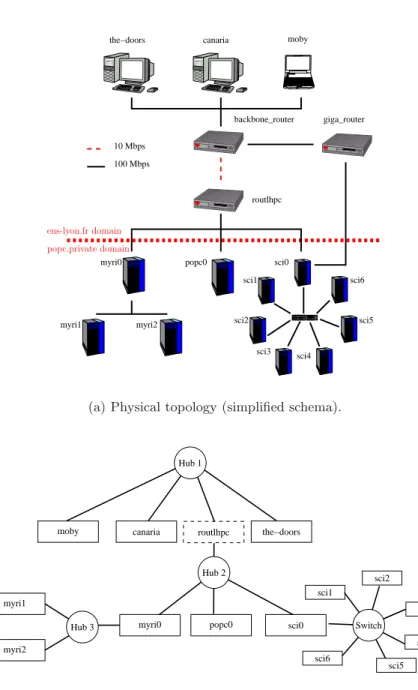
Figure1presents the results of ENV running on the ENS-Lyon network as explained in next

section. Figure 1(a) shows the physical network topology while Figure 1(b) is the result of

an ENV run. The presented physical topology is simpliﬁed and asymmetric routes as well as used VLANs are not pictured. The pictured eﬀective network view is the one obtained when choosing the-doors as master.

We can see that some routers are suppressed from the eﬀective network view. In fact, the remaining ones where needed because of route asymmetry. Besides, ENV reports the fact that popc0, myri0 and sci0 are on a 100 Mbps hub, whereas links to reach popc0 and myri0 from the-doors must go trough a bottleneck at 10 Mbps.

4.2 Example of execution

We now detail how ENV collects the data, taking the mapping of the ENS-Lyon network as example. This process can be split in two parts: the ﬁrst is independent from the choice of the master, while the other is not.

(10)

backbone_router canaria moby the−doors routlhpc giga_router 10 Mbps 100 Mbps myri1 myri2 popc0 sci0 sci1 sci2 sci4 sci5 sci6 myri0 sci3 00 00 00 11 11 11 00 00 00 11 11 11 popc.private domain ens-lyon.fr domain

(a) Physical topology (simpliﬁed schema).

moby canaria routlhpc the−doors

myri0 popc0 sci0

sci3 sci2 sci4 sci5 sci6 sci1 myri1 myri2 Hub 3 Switch Hub 2 Hub 1

(b) Eﬀective topology from the-doors’s point of view.

(11)

4.2.1 Master-independant data collection

This phase is itself split in 3 parts.

4.2.1.1 Lookup

During this phase, the core GridML is created, using provided hostnames. For example, on

canaria and moby we would have the following GridML :

<?xml version="1.0"?> <GRID>

</LABEL> </MACHINE> <MACHINE>

</LABEL> </MACHINE> </SITE> </GRID>

The GRID is divided in SITE nodes, for which each machine is represented by a MACHINE node.

4.2.1.2 Extra information gathering

Information on hosts such as Operating System or processor type are acquired. It is possible to extend ENV to capture any information about hosts relevant to the planned use.

</LABEL>

</MACHINE>

4.2.1.3 Structural topology

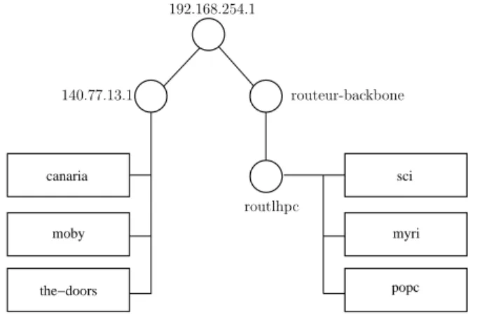
This constitutes a ﬁrst approximation of the topology builded with traceroute, and used to guide the active tests of latter phases. Each host involved in the mapping reports the path used to get out of the Grid by targeting a traceroute to a well known external destination. The part within the mapped network is used to build a tree such as the one presented in

Figure2. Hosts using the same route to get out of the studied network are clustered together

(12)

moby the−doors canaria popc myri sci routlhpc routeur-backbone 192.168.254.1 140.77.13.1

Figure 2: Structural topology: the initial tree in ENV.

In our example, a test on canaria, moby, the-doors, myri, popc and sci gives the following GridML :

This tree is not suﬃcient, because it does not show for example which links are shared and which are switched. For this, a few more tests will be done, that depend on the master’s viewpoint.

4.2.2 Eﬀective topology: Master-dependent data collection

The second part of the data collection depends on the chosen master. These measurements can be seen as successive reﬁnements of the structural view of the network. This allow to generate a new tree containing the so-called ENV networks, which contain the critical information in our context about the layer 2 topology.

Most of these experiments use thresholds to interpret the measurement results. The value of this thresholds may have a great impact on the mapping results, and where determined experimentally and empirically by the ENV authors.

(13)

the-doors any host

This experiment splits the clusters to group machines having a compara-ble connexion to the master. The bandwidth between the master M and

any host A is measured separately. Then, clusters previously made are divided into groups with similar bandwidth. If the bandwidth ratio between two hosts exceeds the threshold of 3, their cluster is split to separate them.

4.2.2.2 Pairwise host bandwidth

the-doors

cluster

This experiment splits the clusters based on how the connexion between their members and the master (M ) is shared. For that, for each pair of machines A and B in each cluster, the bandwidths of M A and M B are tested when the transfers occur concurrently.

This measurement is then compared to the

band-width as measured in the previous step. If the ratio

Bandwidth(M A)/Bandwidthpaired(M B)(M A) is below a threshold of 1.25, A is declared in-dependent of B and the cluster is split to separate those hosts.

4.2.2.3 Internal host bandwidth

cluster

For each cluster, bandwidth is measured between any pair of machine, within this cluster. This allows to set the local band-width parameters for a given cluster. This may be useful for clusters where local bandwidth is diﬀerent from bandwidth achieved between the cluster and the master. For example in ENS-Lyon, the route from the-doors to the popc cluster goes

trough a 10 Mbps bottleneck, whereas popc is on a local 100Mbps hub.

4.2.2.4 Jammed bandwidth

the-doors

cluster

For each cluster, the bandwidth to the master is measured while a transfer between two other hosts of that cluster oc-curs. This measure is repeated 5 times, and the average of the

ratio Bandwidth/Bandwidthjammed is computed.

If the average is below the threshold of 0.7, the cluster is reported to be on a shared link. If the average is above the

threshold of 0.9, the cluster is reported to be on a switched link. If the average is between those two thresholds, data gathering about this cluster stops since the values are not signiﬁcant enough.

Here is for example the description of a switched network created after this test (the sci cluster):

...

(14)

</NETWORK> ...

All these reﬁnements allow us to determine whether structural networks are switched or shared based upon bandwidths observed between hosts. This information has a great impact

on the NWS deployment, as explained in section 5.

4.3 Known ENV issues

We describe in this section some problems that we encountered with ENV, and solutions that we propose when applicable.

Bandwidth waste The ENV tests are still introducing a significant bandwidth consump-tion. It cannot be prevented since active probes are needed to infer layer 2 informations without relying on specific tools which may not be available. The point is that a given plat-form needs to be mapped with ENV only once, and the results can then be shared between different people. For example, administrators could publish the mapping of their network as reported by ENV, so that any user can use it without redoing the mapping.

Firewalls Since firewalls prevent communications, it is naturally not possible to do all the needed tests when some machines are firewalled. We solved this issue by running ENV on each side of the firewall, and merging the results afterward. For example, the ENS-Lyon

network is split in two sub-domains as depicted on Figure1(a). The hosts sci1, sci2, . . . cannot

communicate with the outside world, but they are connected to sci0, popc0 and myri0, which can act as gateways. We therefore launched ENV on both sides of popc0 separately.

The following merge is quite simple: a new GridML structure containing both sites (here ens-lyon.fr and popc.private) is created, and the aliases of hosts belonging to both sites are provided. This operation is often as simple as a ﬁle concatenation. The only information the user has to provide is the several aliases of the gateways machines depending on the considered site. In our example, the aliases were:

popc.ens-lyon.fr popc0.popc.private myri.ens-lyon.fr myri0.popc.private sci.ens-lyon.fr sci0.popc.private

Which leads to the following GridML : <GRID>

(15)

Machines without hostname When traceroute are performed in the first stage, the hosts are said to be in the same domain (and thus, considered for the experiment) based on their full qualified domain name. But some hosts have no configured name and their IP appear in the traceroute result. Since it was the case in our network, we modified ENV to simply use IP address class [11] if IP resolution fails.

We also modiﬁed ENV to support non-routable IPs. Those addresses are routables only from the local network and thus are always part of the local domain. They should therefore be kept in the ﬁrst phase of the mapping. For example the root of the structural topology

depicted on Figure 2 is a non-routable IP, but dropping this information may badly impact

the mapping quality.

Asymmetric routes The physical network in ENS-Lyon is more complex than Figure1(a) depicts. Indeed the route between the-doors and popc goes trough a 10 Mbps link, whereas in the other direction it is on 100 Mbps links only. According to [17], this situation, even if quite queerly, is rather common on Internet. Since ENV bandwidth tests are conducted in only one way, the system cannot detect such problems. Solving this would imply almost a complete rewrite of ENV tests and is still to do.

Likewise, networks are usually packet driven and we cannot guarantee that the path between two given hosts always follows the same route. However, since ENV is mainly used to map local networks, we assume that this is the case for the duration of the experiment, or at least, that global measurements are not too sensitive to this variation.

Dropped traceroute According to [12], many modern routers no longer respond to trace-route packets. This may not be a great problem for ENV, because clusters are still split based on bandwidth measures made in preceding tests. So, structural networks may be affected by this, but not the final result. Nevertheless, this would make measures longer, given that for clusters discovered in first stage, all possible pairs of hosts are tested. Bigger clusters means more measures in the second stage, hence more execution time.

Implementation portability ENV is implemented in the Python programming language, which seems at the ﬁrst glance to be a good portability compromise since the same code should work on all platform with no modiﬁcation.

The experimental reality is rather diﬀerent, and running ENV on a rather homogeneous set of machines (all machines were i386 Linux boxes) revealed to be a challenging problem. We had of course to install Python on all machines: this programming language may be

(16)

rapidly spreading, it is not yet installed on computational servers by default. Moreover, ENV also requires extra libraries which in turn requires extra precaution to compile their Python bindings to become accessible from this programming language..

Optimists will consider that this issue should not last for long as Python is spreading more and more quickly. Pessimists will object that Python is also rapidly evolving and that the backward compatibility is not provided across the versions, which will cause even further problems in the future. Moreover, a lot of scripting languages may constitute a portability layer, but determining which one will become dominant in the future and which one will survive in the next few years is still very diﬃcult. Another solution would be to rewrite ENV in C or equivalent, but the resulting program would be more complex and harder maintain since Python is a high level programming language.

Reliability and accuracy Even if ENV provides some bandwidth estimations, their ac-curacy is not crucial in our context since NWS is to be deployed, and provides much more accurate and up-to-date measurements. Qualitative and topological information about the network are therefore much more important than quantitative one.

The first problem is the possible platform evolution: many inter-dependent tests are to be run and they last some time to complete. The results given by ENV may be corrupted if the network load evolves greatly (increasing or decreasing) between tests. There is no solution yet to this problem, except rapidity: the mapping of our platform only last a few minutes, so we assume that the environment is stable enough to provide viable results in those conditions. For bigger platforms. it would be possible to map separately the different parts of the network and then merge the results together, just like we did to map both sides of firewalls.

Moreover, experimental thresholds may be problematic, because they may be speciﬁc to platform characteristics like the media type. They may for example be adapted to LAN, but not to Terabit links. Besides, determining if the thresholds are adapted to the current platform is very diﬃcult.

Link A Cluster 1 Link B Cluster 2 Link C Platform Master

Master/Slave paradigm ENV was designed for mas-ter/slave computing, and this may lead to important informa-tion loss during the mapping. For example, the lateral ﬁgure depicts a Master and two clusters 1 and 2. While the links

A and B (between the master and each cluster) are discovered

by ENV, the link C (between the two clusters) is not because ENV does not make “inter-cluster” tests. This information loss seems to be the price to pay for rapidity, since gathering all information about the network may require a very long time to complete. Indeed, using exactly the same methodology as ENV for a whole mapping would require to ﬁrst drive n∗(n−1)

band-width tests between each couple of hosts {a; b}. Then, it would

require for each pair of link {a; b} and {c; d} to conduct experiments to determine whether

those network path are dependent or not, i.e. whether a transmission on {a; b} impacts the

bandwidth of {c; d} or not. This naive algorithm would not scale at all because of the

band-width and time consumed. Considering that collecting information about two given links lasts half a minute (which is reasonable since the network needs to stabilize between each experiments), the whole process would last about 50 days for 20 hosts. That is why ENV

(17)

does not try to completely map the network, but only focuses on a view of the network from a given point of view.

5 Deploying the NWS using ENV

Most common Grid testbeds are constituted of several organizations inter-connected by a wide area network, each of them sharing local resources (like clusters) interconnected by local area network with the others. The resulting platform is a WAN constellation of LAN resources. The most natural solution to satisfy all constraints is then to set up a hierarchical monitoring infrastructure, where intra-site connectivity is tested separately from the inter-site one. If needed, this hierarchy can contain more than two levels, and intra-cluster connectivity would be measured separately from the inter-cluster one.

5.1 Deployment planning

This section presents a simple algorithm to plan the NWS deployment using the data gathered by ENV. For each network or subnetwork discovered by ENV, our deployment plan contains at least two cliques:

• If the network is shared, its hosts are supposed to be on the same physical link, so the

latency and bandwidth of one couple of hosts is representative for any possible couple. The intra-network connectivity is then measured by a clique containing two arbitrary chosen hosts.

Note that even if this is suﬃcient to gather the needed information, this method reveals a NWS shortcoming: it is currently not possible to inform the system that the connexion between two hosts (AB) is representative of the connexion between two other hosts (CD), and the user has to keep track of this to ask NWS about (AB) when he wants to retrieve the characteristics of (CD).

• If the network is switched, the network characteristics between each host pair are

inde-pendents and could be measured separately, but each host must be involved in at most one measurement at a given time. That is why we deploy a NWS clique containing all the hosts to make sure that only one measurement will occur at the same time on the given group of hosts.

Note that using a clique is a bit too restrictive. On a switched network, the tests AB and CD would not collide if they involve diﬀerent hosts, i.e. if {AB} ∩ {CD} = ∅. On the other hand, the only drawback of allowing at most one test over the group at the same time is that the frequency of a given test between two given hosts slightly decrease.

The resulting deployment plan for the ENS-Lyon network is depicted on Figure 3. The

sci cluster is switched, so we pick all its machines to form a new clique, whereas the myri

cluster is shared, so we pick only two hosts for the local clique (myri1 and myri2 ). myri0 and popc0 were chosen to test the network characteristics on Hub 2 while moby and canaria are used to test the Hub 1. The connection between canaria and popc0 is used to test the connexion between these hubs.

(18)

moby canaria routlhpc the−doors

myri0 popc0 sci0

sci3 sci2 sci4 sci5 sci6 sci1 myri1 myri2 Hub 3 Switch Hub 2 Hub 1

Figure 3: NWS deployment plan in ENS-Lyon.

5.2 Deployment plan application

Once the deployment plan has been computed, another challenging issue is to actually apply it, and launch the several parts of NWS on the different hosts with the right options. In-deed, the official version of NWS offers very few support to process management and global configuration and one have to manually ssh to the right host, and pass manually the right option on the command line of each NWS process.

To solve this issue, we realized a NWS manager program using a configuration file shared across all involved hosts and applying the local parts on each hosts. The actual deployment of NWS is then as easy as dispatching the configuration file to the hosts (using for example NFS), and running the manager on each machines.

Our implementation is still fallible since it is implemented in the Perl scripting language and thus needs a proper interpreter on all involved hosts.

6 Conclusion

The Network Weather Service constitutes a de facto standard of Grid platform monitoring tool used by major Grid PSEs. Unfortunately, deploying this tool remains tedious since no automatic tool is provided by default, and since the manual deployment requires accurate knowledges both about the current network on which the tools are to be deployed and about the NWS internals.

The main diﬃculty remains to accurately map the target network, and ENV seems to be the better suited tool to our needs among the existing ones. In contrary to SNMP-based tools or pathchar, it does not require any speciﬁc privileges to run. This is very important on a Grid constituted of several organizations sharing their local resources but possibly not willing to give extra privileges to the Grid users on their network. In contrary to simple solutions based on ping or traceroute, ENV is also able to quantify how each detected network is shared among several concurrent transfers, which reveals to be a crucial information to achieve a proper NWS deployment. After characterizing the constraints a good NWS deployment should satisfy, we proposed a simple algorithm to deduce a deployment plan from the information provided by ENV.

(19)

This paper relates an experiment to automatically deploy NWS on our lab’s network using our methodology. This experiment was fortifying since it allowed us to identify several shortcomings and needs both in the ENV and NWS tools.

The ENV tool only provides a tree view of the network to simplify and speed up the mapping process. This is well adapted to a master/slave paradigm, but this is too limited in the general case since it will overlook some transversal links between leafs of the tree. ENV also considers that the routes are symmetric and only test them in one direction.

According to [17], this simpliﬁcation is over-optimistic. Finally, ENV is implemented in

the Python scripting language and depends on speciﬁc extensions of this language. Since this language uses a virtual machine to make the code portable, this seems to be a good portability compromise, but the experimental reality proved to be rather diﬀerent, and installing all ENV dependencies on the target machines proved to be the mostly tedious task of the mapping.

The NWS does not provide process managing facilities, and we realized a prototype of NWS manager implemented in Perl (and thus having the same portability issues than ENV) which can locally apply the deployment plan to the current machine.

Another concern revealed by this experiment involves the NWS protocol used to make sure that experiments will never collide on a given resource (which would lead to wrong measurements). It makes sure that only one pair of hosts from a given group will conduct an experiment at a given time. But on a switched network, more than one experiment may be authorized if the hosts involved in each experiments are diﬀerent. That is to say that a possibility to lock hosts (and not networks) is still needed. Moreover, if the network is shared (using an hub), testing the connexion capacities between each pair of host will be the same, and testing one pair is enough. Unfortunately, NWS is then unable to substitute automatically the characteristics of the tested pair when another pair is asked. More generally, NWS is unable

to aggregate measurement results when no direct experiment were conducted. However,

reducing the number of direct measurements is a must to ensure the system scalability.

References

[1] A. Bierman and K. Jones. Physical topology mib. RFC2922, september 2000.

[2] H. Burch, B. Cheswick, and A. Wool. Internet mapping project.

http://www.lumeta.com/mapping.html.

[3] Eddy Caron, Fr´ed´eric Desprez, Franck Petit, and Vincent Villain. A Hierarchical

Re-source Reservation Algorithm for Network Enabled Servers. In IPDPS’03. The 17th

International Parallel and Distributed Processing Symposium, Nice - France, April 2003.

[4] H. Casanova and J. Dongarra. Using Agent-Based Software for Scientiﬁc Computing in the Netsolve System. Parallel Computing, 24:1777–1790, 1998.

[5] Mathijs den Burger, Thilo Kielmann, and Henri E. Bal. TOPOMON: A monitoring tool for grid network topology. In International Conference on Computational Science (ICCS

2002), volume 2330, pages 558–567, Amsterdam, April 21-24 2002. LNCS.

[6] P. Dinda, T. Gross, R. Karrer, B Lowekamp, N. Miller, P. Steenkiste, and D. Sutherland. The architecture of the remos system. In 10th IEEE International Symposium on High

(20)

[7] Allen B. Downey. Using pathchar to estimate internet link characteristics. In

Mea-surement and Modeling of Computer Systems, pages 222–223, 1999. Available at http://citeseer.nj.nec.com/downey99using.html.

[8] I. Foster and C. Kesselman (Eds.). The Grid: Blueprint for a New Computing

Infras-tructure. Morgan Kaufmann, 1999.

[9] I. Foster and C. Kesselman. Globus: A Metacomputing Infrastructure Toolkit.

Interna-tional Journal of Supercomputing Applications, 11(2):115–128, 1997.

[10] P. Francis, S. Jamin, C. Jin, Y. Jin, D. Raz, Y. Shavitt, and L. Zhang. Idmaps: A global internet host distance estimation service. IEEE/ACM Transactions on Networking, oct

2001. Available athttp://citeseer.nj.nec.com/francis01idmaps.html.

[11] S. Kirkpatrick, M. K. Stahl, and M. Recker. RFC 1166: Internet numbers, July 1990. Obsoletes RFC1117, RFC1062, RFC1020 Status: INFORMATIONAL. Available at

ftp://ftp.math.utah.edu/pub/rfc/rfc1166.txt.

[12] Bruce B. Lowekamp, David R. O’Hallaron, and Thomas R. Gross. Topology discovery for large ethernet networks. In ACM Press, editor, ACM SIGCOMM 2001, pages 237–248,

San Diego, California, 2001. Available athttp://citeseer.nj.nec.com/500129.html.

[13] D. McPherson and B. Dykes. RFC 3069: VLAN aggregation for eﬃcient IP

ad-dress allocation numbers, February 2001. Status: INFORMATIONAL. Available at

ftp://ftp.math.utah.edu/pub/rfc/rfc3069.txt.

[14] Nancy Miller and Peter Steenkiste. Collecting network status information for network-aware applications. In INFOCOM’00, pages 641–650, 2000.

[15] H. Nakada, M. Sato, and S. Sekiguchi. Design and Implementations of Ninf: towards a Global Computing Infrastructure. Future Generation Computing Systems,

Metacomput-ing Issue, 15(5–6):649–658, Oct. 1999.

[16] E. Ng and H. Zhang. Predicting internet network distance with coordiantes-based

ap-proaches, 2001. Available at citeseer.nj.nec.com/article/ng01predicting.html.

[17] Vern Paxon and Sally Floyd. Why we don’t know how to simulate the internet. In

Proceedings of the Winder Communication Conference, December 1997. Available at

http://citeseer.nj.nec.com/article/floyd99why.html.

[18] Vern Paxson. Measurements and Analysis of End-to-End Internet Dynamics. PhD thesis, University of California, Berkeley, 1997.

[19] Y. Rekhter and T. Li. A border gateway protocol 4 (bgp-4). RFC1771, March 1995. [20] Srinivasan Seshan, Mark Stemm, and Randy H. Katz. SPAND: Shared passive network

performance discovery. In USENIX Symposium on Internet Technologies and Systems,

1997. Available athttp://citeseer.nj.nec.com/seshan97spand.html.

[21] Gary Shao, Francine Berman, and Rich Wolski. Using eﬀective network views to

promote distributed application performance. In International Conference on

Paral-lel and Distributed Processing Techniques and Applications, June 1999. Available at

(21)

[22] R. Wolski, N. T. Spring, and J. Hayes. The Network Weather Service: A Distributed Resource Performance Forecasting Service for Metacomputing. Future Generation

Com-puting Systems, MetacomCom-puting Issue, 15(5–6):757–768, Oct. 1999.

[23] Rich Wolski, Benjamin Gaidioz, and Bernard Tourancheau. Synchronizing network

probes to avoid measurement intrusiveness with the Network Weather Service. In 9th