AVIS
Ce document a été numérisé par la Division de la gestion des documents et des archives de l’Université de Montréal.
L’auteur a autorisé l’Université de Montréal à reproduire et diffuser, en totalité ou en partie, par quelque moyen que ce soit et sur quelque support que ce soit, et exclusivement à des fins non lucratives d’enseignement et de recherche, des copies de ce mémoire ou de cette thèse.
L’auteur et les coauteurs le cas échéant conservent la propriété du droit d’auteur et des droits moraux qui protègent ce document. Ni la thèse ou le mémoire, ni des extraits substantiels de ce document, ne doivent être imprimés ou autrement reproduits sans l’autorisation de l’auteur.
Afin de se conformer à la Loi canadienne sur la protection des renseignements personnels, quelques formulaires secondaires, coordonnées ou signatures intégrées au texte ont pu être enlevés de ce document. Bien que cela ait pu affecter la pagination, il n’y a aucun contenu manquant.
NOTICE
This document was digitized by the Records Management & Archives Division of Université de Montréal.
The author of this thesis or dissertation has granted a nonexclusive license allowing Université de Montréal to reproduce and publish the document, in part or in whole, and in any format, solely for noncommercial educational and research purposes.
The author and co-authors if applicable retain copyright ownership and moral rights in this document. Neither the whole thesis or dissertation, nor substantial extracts from it, may be printed or otherwise reproduced without the author’s permission.
In compliance with the Canadian Privacy Act some supporting forms, contact information or signatures may have been removed from the document. While this may affect the document page count, it does not represent any loss of content from the document.
Reconstruction of the surface of the Sun from
stereoscopie images
par
Vlad - Andrei Lazar
Département d'informatique et de recherche opérationnelle Faculté des arts et des sciences
Mémoire présenté à la Faculté des études supérieures en vue de l'obtention du grade de
Maître ès sciences (M.Sc.) en informatique
Décembre, 2007
Ce mémoire intitulé :
Reconstruction of the surface of the Sun from stereoscopie images
présenté par
Vlad - Andrei Laûir
a été évalué par un jury composé des personnes suivantes:
Mémoire accepté le Max Mignotte (président-rapporteur ) Sébastien Roy (directeur de recherche) Pierre Poulin (membre du jury)
Cette thèse s'intéresse à la reconstruction stéréoscopique dans des environnements contenant des objets transparents, comme la couronne solaire. Les données pour ce projet, images stéréoscopiques du soleil, ont été fournies par la NASA grâce à la mis-sion STEREO. Ce mémoire propose une nouvelle méthode de rectification sphérique ainsi qu'un nouvel algorithme pour la reconstruction dense sans aucune hypothèse préalable sur la forme ou la transparence des objets dans la scène.
Premièrement, les paramètres des caméras sont estimés, et une étape de raffine-ment suit pour obtenir un aligneraffine-ment presque parfait entre les images. Dans l'étape suivante, les images sont rectifiées pour réduire l'espace de recherche de trois à deux dimensions. Les densités le long des lignes épipolaires sont ensuite estimées.
La reconstruction des scènes transparentes est encore une problème ouvert et il n'y a pas de méthodes générales pour résoudre la transparence. Les applications pour cet algorithme sont nombreuses, comme la reconstruction des traces de fumée en soufflerie, le design optimal des chambres à combustion, la realité augmentée, etc. Mots clés: vision par ordinateur, rectification, stéréoscopie, transparence, esti-mation de profondeurs multiples, soleil, physique solaire
This thesis concentrates on the stereoscopic reconstruction of environments con-taining transparent objects. The data used to test the algorithms is graciously pro-vided by NASA through the STEREO mission. This thesis proposes a new spherical rectification technique as well as a dense reconstruction algorithm without making any prior assumptions on the shape or transparency of objects inside the scene.
Firstly, the camera parameters are estimated, following a refinement step to get seamless alignment between images. In the next step the images get rectified in order to be able to restrict the search space to 2D rather than the full 3D. Afterwards the density at along each epipolar line gets estimated.
The reconstruction of transparent scene is stilllargely an open problem and there are no general methods to deal with transparency. The applications of such an algo-rithm are numerous, ranging from reconstruction of smoke trails inside wind tunnels, optimal design of combustion chambers, augmented reality, etc.
Keywords: computer vision, rectification, transparency, stereoscopy, multiple depth estimation, Sun, solar physics
List of Figures
Chapter 1: Introduction 1.1 Outline . . . .
Chapter 2: Astronomical and solar imaging 2.1 STEREO mission .
2.2 Coordinate systems 2.3 Influence of magnetic field
Chapter 3: 3D Geometry and reconstruction 3.1 Homogeneous coordinat es
3.2 Camera models 3.3 Radial distorsion 3.4 Planar homographies
3.5 Stereoscopie reconstruction . 3.6 Satellite camera calibration
Chapter 4: Rectification 4.1 Related work . . . 4.2 Planar rectification 4.3 Cylindrical rectification. 4.4 Spherical rectification . 4.5 Sorne results . . . . 111 1 4 5 8 9 15 20 20 21 24 26 26 33 39 39 39 42 43 50
5.2 Image formation model . 5.3 Problem statement 5.4 Reconstruction volume
5.5
The minimization problem 5.6 Cost functions . . . . . ~ ..Chapter 6: Res ult s 6.1 Synthetic results 6.2 Solar images . . .
Chapter 7: Discussions and conclusions 7.1 Further· developments . Bibliography 11 58 60 60 62
64
6868
73 7980
821.1 Coronal loops captured by the TRACE mission 284A
2.1 The 4 wavelengths captured by STEREO . . . . 2.2 Image of the Sun as seen by STEREO-B in the 195A
2.3 Sun seen from the two STEREOs . . . . 2.4 Celestial and ecliptic planes together with the equinoxes 2.5 Heliocentric cartesian coordinate system
2.6 Magnetogram provided by MDI . . . 2.7 Linear force free magnetic field reconstruction
3.1 Pinhole camera projection model 3.2 Radial distorsion [1] . 3 7 9 10 12 13 17 19 22 25 3.3 3.4 3.5 Triangulation . . . . 27
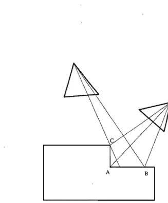
Occlusions: A is partially occluded, B is fully visible and C is an occluder 29
Epipolar geometry . . . . 29
3.6 Correspondence of x and x' on an epipolar line . 31
3.7 Dynamic programming . . . 32 3.8 Tsukuba dataset: Left - direct search, Right - dynamic programming 32
4.1 Original and rectified epipolar lines . . . 40
4.2 Epipolar li ne with spherical rectification 44
4.3 Sphere with corresponding circle. . . 46
4.4 Two dimensional circle tangent problem. 47
4.6 4.7 5.1 5.2 5.3 5.4 6.1 6.2 6.3 6.4 6.5 6.6 6.7
Cartesian discretization of a circle
Top: original image, Middle: uniform sampling, Bottom: non uniform sampling . . . .
Density sheet reconstructions generated by two orthogonal views . Reconstruction volume . . . .
Reconstruction grid. Gray is valid region .. N orm functions . . . .
Ground truth. Sparsity of 1.31 .
l2 norm minimization. Sparsity of 3.28
Iterative minimization with the weighted
h
norm. Sparsity of 1.31 Minimization with the non-convex sparsity measure. Sparsity of 0.74 Torus dataset: top - the two input views, bottom - sideways view Torus reconstruction with l2 norm . . . .Torus reconstruction with iterative minimization .
49
51 56 61 62 66 69 69 70 70 72 72 736.8 Left: STEREO A, Right: STEREO B. . . . 74
6.9 Top and oblique views of the reconstruction 75
6.10 Left: STEREO A, Right: STEREO B. . . 76
6.11 Top and oblique view of the reconstruction 77
6.12 Left: Reconstruction of the surface of the Sun, Right: STEREO A minus the surface showing just the moving parts. . . . . 78
INTRODUCTION
The field of machine vision aims at developing algorithms that mimic functions of the human visual system. U sing d!1ta from sensors (imaging, range scanners, etc.), the algorithms are trying to get information about the surrounding physical world. Each of the sensors observes merely just a "projection" of the real world so this information must be merged to recover the world coordinates. Out of the machine vision problems, the one that received most of the attention is 3D reconstruction. Applications are numerous, ranging from metrology, navigation and adaptive multimedia systems.
In this thesis we attempt to develop a reconstruction scheme for solar cororial loops using extreme ultraviolet images taken by the STEREO mission, while making just standard smoothnessjsparsity assumptions. For the first time we have simulta-neous satellite images from two vantage points using identical instruments. Previous attempts at reconstruction used single vantage' point images spaced in time, using the solar rotation to provide different views of the features.
The STEREO mission will provide an important tool to validate the theoretical models of magnetic fields and plasma flows on the Sun. The holy grail of solar physics is the accurate prediction of the space weather, which has a strong influence on our day to day activities. The coronal loops have a major influence on this phenomena. The loops on the surface of the Sun sometimes erupt outside the corona and escape the Sun's gravity. This creates the aurora Borealisj Australis and disrupts satellites and radio communications. Prediction of such phenomena relies on accurate 3D models of such loops, which is the main concern of this thesis.
There are multiple approaches to the 3D reconstruction problem. The simplest of which, uses pixel matching techniques along epipolar lines and together with the projection model, one can triangulate the world 3D position of each pixel. In this meth6d one chooses a reference view and the resulting reconstruction is from this point of view. An alternate, but similar method, is volumetrie reconstruction. The reconstruction volume 'gets discretized into volume elements, and the value at each voxel is dietated by an average of the pixel values from all views where the voxel is visible. This can accommodate an arbitrary number of views. U sually a voxel is either fully transparent or opaque leading to a single depth for a pixel inside the images. The success of this method is strongly infiuenced by our occlusionjvisibility modelling.
Another family of methods, used commonly in medical imaging, is the tomographie
reconstruction. Given a large number of projections of the object one can reconstruct the object with low error. Normally we will settle for a few hundred projections in order to obtain good results. This method used certain properties of the Fourier transform of the projections to perform the reconstruction. Usually an orthographie projection model is assumed.
The current algorithms cannot reconstruct reliably transparent env'ironments un-less an unreasonable number of input images is used or an a priori knowledge of the shape of objects is available. We will have to cope with as 1ittle as two or three images (if we use SOHO images as well). The solar loops are short lived phenomena, thus preventing us from using images taken at different instances of time.
The method proposed in this thesis is a hybri~ between the volumetrie and to-mographie reconstructions: like the toto-mographie reconstruction we are looking for a certain "matter density" inside each voxel, but the original rectified images are used directly rather than the Fourier transform of its projection. The problem poses itself as a constrained minimization problem. The constraints are provided by the avail-able views together with the corresponding projection models. The function to be
Figure 1.1. Coronal loops captured by the TRACE mission 284A.
minimized, provides sorne kind of regularization, helping us to impose certain prop-erties of the solution. The problem is massively underconstrained: given a uniform discretization of n in each dimension, our reconstruction volume has n3 cells (vox-els ) with O(n2
) equations given by the views). This algorithm will be applied on solar coronal loops captured by STEREO (Fig. 1.1). The problem of transparent stereo matching is extremely challenging and there exists no current solution which is satisfactory. Because of this the results presented here are far from perfecto
A secondary contribution of this project is a rectification scheme named spherical
rectification, which has all the good properties of state of the art rectification methods such as the ability to rectify any camera configuration outputting a finite image size, but is particularly useful for objects which are on spheres.
1.1 Outline
The thesis is organized as follows: in chapter 2 we present a brief history of solar observation, sorne current open research topics and a bit of physical background that will be useful in the later parts. In chapter 3 we introduce the standard 3D reconstruction toolkit. Chapter 4 introduces the fundarnentals of rectification as well as sorne srnall results of our own rectification rnethod. In chapter 5 we introduce the standard. rnethods to reconstruct transparent environrnents and our proposed rnethod. Chapter 6 presents sorne results of our reconstruction with both synthetic and read data, and in chapter 7 we suggest sorne future irnprovernents.
ASTRONOMICAL AND SOLAR IMAGING
The Sun has been a source of fascination for mankind before the dawn of his-tory. Numerous historical discoveries stand witness that prehistoric people had basic knowledge of solar system planetary cycles.
Tt was not until' arouhd the year 1600 that the first Earthbound solar telescope was built by Galileo Galilee. He was the first to observe the solar dark spots. During the
19th cent ury, the German astronomer Heinrich Schwabe observed that the number of spots increases and decreases with time. He was the first to observe that the period of this solar act}vity oscillation is about Il years.
Probably the greatest contribution to solar observations was brought by George Ellery Hale in the 20th cent ury. He discovered that the sunspots were cooler than the surrounding matter, and thus darker (the magnetic field inside the sunspots is strong enough to prevent convection, so hot matter from the inner Sun cannot reach the surface). Another important contribution was the observation that every 11 years the solar magnetic poles get reversed, giving birth to a'more fundamental solar cycle of 22 years[2].
Since the beginning of the space age, the knowledge about the Sun has increased exponentially. This was powered by both recent theoretical physics and technological developments. Using airbornejspaceborne observatories has improved the quality of data by removing the effects of the atmosphere that could corrupt the data. Ob-servations of certain 'wavelengths, such as X rays, are impossible inside the Earth's
atmosphere because of its high absorption rate.
The motivation for the special interest in the Sun is fairly straightforward: it is our only source of high resolution data of the physical processes inside stars. The
activity on the Sun has a strong influence on our day to day activities as well, giving us more pragmatical reasons for its study. High energy particles ejected by the Sun into outer space - the solar wind - change on a global scale the Earth's climate, the most visible effect being Aurora Borealis/ A ustralis. Other bad effects include disruption of geostationary satellites, pipelines, electrical power grids and increased levels of radiation. The generation of solar wind follows an extremely complicated mechanism, not entirely known.
The Sun provides a lot of information about processes that are not easily repli-cated by man made experiments. In elementary particle and nuclear physics the benefits were numerous. With the help of solar data, about 30 years ago the
neutri-nos were discovered. Up until the year 2002 there was a major discrepancy between the predicted and observed neutrino amounts. Finally two new types of neutrinos have been discovered (with muchlower probability of interaction).
The bulk part of the solar energy is generated thorough the eND cycle (Carbon, Nitrogen, Oxygen), in which stars convert through fusion Hydrogen into Helium, a phenomenon which is still not totally understood.
In the field of plasma physics the most important contributions were wave prop-agation and magnetic field generation.
One of the largely open problems is the coronal heating problem. The solar corona is the outer most atmosphere. This extends from Rsun to about 2 - 3 solar radii. The mystery behind the corona pertains to its heating mechanism. It is about 200 times hotter than the photosphere - the next inner layer. The temperature of the corona rises from 5 0000 K
to about 1 000 0000 K
within 200 000 Km. There is still no generally accepted theory regarding the energy transfer mechanisms from the photosphere to the corona. The two most prevalent theories are the wave transport
theory and the magnetic reconnection theory. The second one has the greater support and we will base our investigations on it. In short this theory claims that the heating is due to the magnetically induced electrical currents. When magnetic fields change
Figure 2.1. The 4 waveIengths captured by STEREO
topology (they merge or divide) a certain amount of energy gets released. In our project we will try reconstructing these field lines.
Because of the extreme temperature most of the matter is ionized. This is fortu-nate since this matter will gather around the magnetic field. The equation of motion for a charged particle inside magnetic field is given by the Lorentz equation:
--+ --+--+
F=q·VxB (2.1)
where q is the particle charge, V is its velocity and B is the magnetic field. Since there is a cross product, the particle will follow a helical motion around the field line. These particles provide an outline of the magnetic field, otherwise invisible (Fig 1.1). For more detailed information on solar and stellar phenomena please refer to
[3-6].
2.1 STEREO mission
In Deeember 2006, NASA launched its third Solar Terrestrial Probe called STEREO (Solar TErrestrial RElations Observatory). The mission consists of two identieal probes orbiting around the Sun, one in front and the other trailing behind the Earth, providing the first true stereoscopie view of the Sun.
The whole mission was designed to provide data for a period of 5 years with its main scientific objective being the better understanding of CMEs (Coronal Mass Ejections). CMEs are important to study since they have a direct impact on our day to day life. Onee they escape the solar gravitational field they turn into solar wind and can disrupt satellites orbiting Earth, telecommunieations, and even the terrestrial electrical power grids.
The mission carries a broad range of instruments. This project will be using the instruments contained in the SECCHI package (Sun Earth Connection Coronal and Heliospheric Investigation). Each satellite contains a EUV (extreme ultra violet) imager that takes images in the wavelengths of 171, 195,284 and 304 Â. Sinee different emission lines get formed at different temperatures, different images provide insight at different depths inside the Sun (Fig. 2.1), ranging from Rsun, up to approximately
2Rsun·
. The satellites orbit -in a helioeentric trajectory (around the Sun), allowing the satellites to separate more and more as time passes, since one is closer to the Sun and thus moving faster. The current separation between the satellites is about 25° and growing by a rate of about 6° per month. The satellites are situated about 109 meters away from the Sun. The field of view of the satellites is around 1.5°, so the projection model being close to an orthographie camera model.
The'data cornes in the FITS format. This is a general purpose format used in Solar and stellar astronomy, that can handle time series, images, or multidimensional data. The FITS files also contain a header where one can accomodate ancillary information
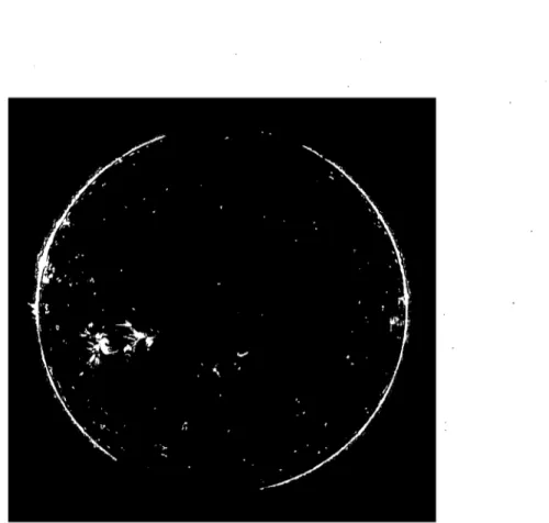
Figure 2.2. Image of the Sun as seen by STEREO-B in the 195J1.
about the conditions in which the data was recorded. SECCHI provides its data as 16bit integer 2D images, (Fig. 2.2).
A more detailed mission description can be found in [7,8].
2.2 Coordinate systems
In order to represent the positions of far astronomical bodies, they are considered as belonging to a sphere of infinite radius - the celestial sphere. In such a system, the parallax is virtually zero. The position of objects in such a system is fully determined by two angle parameters, the right ascension and declination (or galactic latitude and longitude). This sphere has its center located at the center of the Earth and its equator in the same plane as Earth's equator - the celestial equator. In a similar fash-ion coordinates on the surface of Earth are represented by two coordinates, latitude
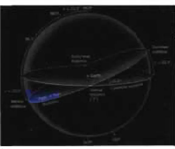
FIIpWe 23. Sun seen from the Iwo STEREOs
ailld longituclle.
Since t.he Sun 1S close enough and the resolution off the observat~ons permits us
to resolve sm aller features, jjt is crucial to introduce a thiFcl! coordinate to accurntely
describe the pheno,rnena occurring on the Sun. As we will see in the chapter' about
camera models (chapte:r 3), the t.hird coo:rdinat.e gets lost due ta proj.€ction onto the
imaging senS0r. Because of this, at least two views a:re needed ta recover the wnole 3D geometry .of phenomena.
Anot.her difficulty in positioning objects onto the Sun is caused by the fact that
there are no stationary points that coul!d serve as re:Derence. The Sun t.ums at
dif-:lferent rates at different latitudes bec-ause of ceNtrifuga] and! magnetic forces. Sorne
coo.rdinate systems will he rotating with respect ta. each other, t.hus it is nec-eS8airy to take also t.jjme into consideration.
2.2.11 World' coordinate sy:stems
Sinee the S'J1S.REO is observi:ng from two very different vantage pOlnts it is neeessary
to ineorporate t.he instrument vl€'W])ofullit (3D position) 1111to the coor-dinate system
(fig. 2.3}.
'Fo be able to :pass from 3D wmldl cooFd1nates to pixeL coordin8ites iim:sidJe images
and orientations of the satellites have to be known (in total 6 parameters, 3 for translations and 3 for rotations). These are the "external" parameters. After this we have to establish a set of 2D transformations that map the coordinates of the Sun to pixel coordinates of the sensors (the "internaI" parameters).
In order to represent the 3D world position of the satellites, the FITS headers provide coordinates in a multitude of coordinate systems. To uniquely define a coor-dinate system we have to pinpoint its origin as well as choose two axes (the third is derived from these axes since we assume a right handed coordinate system). We use heliocentric coordinate systems, so the origin is at the center of the Sun. The most useful orientations of the axes are:
1. Heliocentric Aries Ecliptic
• X axis points towards the First Point of Aries
• Z axis points towards the ecliptic north pole
2. Heliocentric Earth ecliptic
• X axis points towards the Earth
• Z axis points towards the ecliptic north pole
The ecliptic plane is the plane in which the Earth rotates around the Sun. The
ecliptic north pole direction is perpendicular to the ecliptic plane.
The first point of Aries, Fig 2.4, is the point in space where galactic longitude is considered O. This is one of the points where the celestial (Earth's) equator plane intersects the ecliptic plane. Whenever the Sun is in one of these two points, an equinox occurs. The first point of Aries has been chosen as the vernal equinox that occurred in 1950. This points towards somewhere in the Pisces constellation. The first point of Aries moves at a constant rate of about one degree every 71 years. This
Figure 2.4. Celestial
aoo
ecliptic planes togetœ,. with the equinaxesmovement is small enough to be considiered €([j,llstant €onsiclering the typical timeseaIe of observed. solar phenomena, which dœs not usuaIly go o;ver 6 months.
Roth these coordinate systems have the origin at the centere>f the Sun, thus the name - neliocentric. These coordinate systems are used to represent the 3D p'Ûsition of the satellites. The satellites are designed to look towards the center of the Sun, making the remaining 3 rotatie>n parameters known. Details on how te> compute them
will be given in chapter 4.
2.2.2 Image coordinate systems
Ne:>..'t we have to deal with conversion from 3D world coordinates to 2D pixel coordi-nates. This is accomplished by using the helioprojective system. Even though they are full 3D systems, they are not very useful to express real 3D world point as they are mostly tied to the Sun, thus changing fairly rapidly with time. Another charac-teristic that makes then unsuitable for this task is the fact that the observer point of view is not incIuded in the system, making it impossible to compare two images taken from two different locations.
pro-, , , , , R _ -- - ---r-- --- ----r -----r- ---r----, 1 l , , " , , , ,
n
~;;Ci~~
n
n. n
n
n
nt~
;u
f
U~ ;;i~i:;u
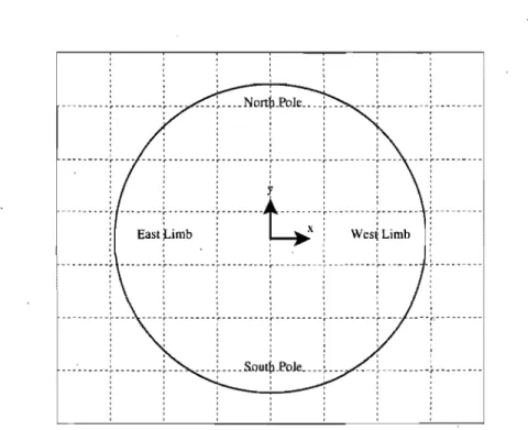
: . ~ : : : , • j , ! - -- - - -r -- - - ---r -- - - ---r-- - --- - --r - ---- ----,..- ---, ' j ! " , , , , , , , , , , , , , , l , l , - - --r - . --- - - - -r - - - -r - - - - -- - - -r- - - -- r ----, , ! j ! , , , , , , , , , ____ ~ ____ s.aut~..Pole--- _~ __ _ , , ,Figure 2.5. Heliocentric cartesian coordinate system
vide the background necessary for the other coordinate systems (Fig. 2.5). In this coordinate system the Z-axis is defined as the observer-Sun line pointing towards the observer. The X-axis is defined perpendicular to the plane defined by Z and the Solar North pole (point around which the Sun rotates). The Y-axis is defined as the cross product between the other two.
2.2.3 Helioprojective coordinate systems
Stars are usually considered far, fiat, virtually positioned at infinity. This is not the case for the Sun, therefore we need a more specialized (accurate) coordinate system to express positions on the surface of the Sun (a sphere).
These coordinate systems mimic the heliocentric coordinates with the difference that their distances are replaced bi angles. The origin of this coordinate system is located at the Sun's center. The Y-axis points towards the solar North pole and the X-axis towards the west solar limb. The solar north/south poles direction is defined
similarily to Earth as the direction perpendicular to the plane of solar rotation. We could define the Z-axis to be the vector product between Y and X, giving us a left handed coordinate system. In practice the third coordinate is fairly useless. The conversion between heliocentric Earth equatorial and helioprojective cartesian coordinates is one to one:
x
~
D(1;0
0 ) <Pxy
~
D(1;0
0 ) <PY(2.2)
(2.3)
(2.4) where x and y are the heliocentric coordinates, <Px and <py are the two helioprojective
coordinates, D is the distance from the observer to solar center. The system assumes implicitly the observation is carried out from Earth. This system is nothing more than a spherical coordinate system analogous to one on the Earth. The system can be extended by adding the 3rd coordinate
ç
=
D - d, where d is the distance between the feature and the observer. In the vicinity of the Sun we can consider thatç
~ z.In practice in order to convert from pixel coordinates to helioprojective system and other way around, we need three extra parameters: the center of the Sun in pixels, a rotation around the satellites Z-axis (the yaw angle) needed to bring the solar north to the top of the picture, and a scale, the number of degrees/pixel.
The only place where the helioprojective coordinate system is used is in solar observations. The astronomers prefer most of the time to replace the true angles by some pseudoangles. The pseudoangles are defined as the projection of a feature onto the z = 0 plane expressed in angles. The pseudoangles vary with the tangent of the real angle. Since the apparent angular size of the Sun, from Earth is around 10
, the
pseudo and true angles differ only at the fifth decimal place.
This approximation is also used when one is observing a spherical surface with a fiat sensor and is called the TAN projection model.
found in [9].
2.3 Influence of magnetic field
The magnetic field is of paramount importance for both theoretical understanding of and data processing. Once we have a model of the magnetic field which is simple enough, we could use it to help us identify features inside the images provided by STEREO.
The full dynamics of matter under magnetic and electric fields is described by a system of 8 coupled partial differential equations called the magneto-hydrodynamic equations (MHD). Since these equations are fairly hard to resolve, an acceptable subset of equations chosen to model the magnetic fi~lds in the corona are the 4 Maxwell equations (the hydrodynamics is considered negligible as the density insidè the corona is minimal):
v·E
- 41fPE(2.5)
v·B
0(2.6)
VxE
1aB
(2.7)
cat
vxB
- - +41fj1aE
cat
(2.8)
where E and B are the electric and magnetic fields, PE is the electric charge den-sity, c is the speed of light and j is the electric current density. We can introduce further simplifications. Since we consider the fields as being in equilibrium, the time derivative terms are negligible.
If we consider that the magnetic field is a potential field, it can be written in terms of gradient of another field B = V
cp.
We get the potential field approximation of the field: V x V .cp
= 0 where B = V .cp,
'12 . B =o.
Standard methods on how to solve· such equations are described in [10]. The solution to the potential field approximation of the problem is the lowest energy configuration possible. This approximation ho Idsonly inside regions on the Sun where activity is very low [11].
For regions with stronger activity, the model of choice is the linear force free model. The equation of this model is
\] x B
=
aB (2.9)With sorne further approximations this becomes \]2 . B
+
a2 B = 0, known as theHelmholtz equation. The parameter a can give us a measure of how unstable the
region is (likelihood of a solar fiare for example). For a = 0 we are back to our
potential field model.
The widely available magnetic data that is available from the MDI mission (Michelson-Doppler Interferometer) provides us with just the normal componentof the magnetic fields on the surface of the Sun. Note however that the magnetic field is a vector function B
=
(Bx, By, Bz) each component depending on (x, y, z). The data avail-able from MDI is BAx, y, Rsun ). We need to propagate the information we have. throughout the whole volume of interest (extrapolate the field) in order to use it at a later stage. In Fig 2.6 we have an example of a magnetogram provided by MDI. Red patches represent fields that exit the surface of the Sun and green patches where fields enter the Sun.
Fourier space methods recently developed in [12-14] provide very efficient ways to extrapolate linear force free magnetic fields. It can be shown that the solution of the Helmholtz equation can be expressed in terms of the Fourier transform of the normal
Figure 2.6. Magnetogram provided by MDI
component:
~
C
mn[7rn (7rmx)
(7rny)
L..; --exp(-rmnz)· a-sin - - cos
-m,n=l Àmn Ly Lx Ly (2.10)
7rm
(7rny) (7rmx)]
-rmn-sm - - cos
-Lx Ly Lx
By(x, y, z) =
~
~ --exp(-rmnz)· Cmn[7rn
a-cos - -(7rmx)
sin - -(7rny)
m,n=l Àmn Ly Lx Ly (2.11)
-rmn-cos - -7rm
(7rny) (7rmx)]
sin-Lx Ly Lx
00 ( ) ( )
7rmx
7rny
L
Cmn exp( -r mnz) . sin---y;; .
sinL
m,n=l y
(2.12)
with Àmn
=
7r2(m2 / L;+
n2 / L;) and r mn=
JÀmn - a, and image sizes are Lx andLy. We can find the coefficients Cmn by choosing z
=
0 in the Bz formula and taking the FFT of Bz(x, y, 0) (our image provided by MDI). In practice we have to do an antisymmetric mirroring of Bz before computing the FFT to get the identical formula:Bz( -x, y) Bz(x, -y) -B(x, y)
-B(x,y)
(2.13) (2.14)Fig 2.7 contains an input image and a few traced lines from the resulting extrapolated magnetic field by the method developed by [14]. Also notice that lines which start very close to the edge of the image exit outside the frame due to periodicity of the dis crete Fourier transform.
Since the coronal loops follow the magnetic field lines, we could use the extrapo-lated field lines to perform a feature based reconstruction of loops.
3D GEOMETRY AND RECONSTRUCTION
This chapter will introduce sorne essential tools used in computer vision that will be used in the chapt ers to come. For a more in-depth introduction refer to [15,16].
3.1 Homogeneous coordinates
The equation of a line in two dimensions is given by: ax
+
by+
c=
0, different choices for a, band c generate different lines. It is also possible to rewrite thisequation by using inner product:x
(a
bc).
y =01
(3.1)
The point (x, y, 1) T on the line· is said to be the homogeneous representation of the 2D point (x,
y).
Clearly if such a point (x,y,
If
belongs to the line, so will the point(kx, ky, kf.
Thus we have an equivalence relation between all points that satisfy the equation of the line (a,b,
c),(x, y,
1)(kx, ky, k), 'ï/k
1:-
O. The concept of homoge-neous coordinates, which are also called projective coordinates, can be expanded in a similar fashion to spaces of higher dimensions. The conversion between homogeneous and Euclidean points is straightforward: just multiply the point by constant such that the last coordinate bec?mes 1 and drop it:(x,y, k)
t'V(x/k, y/k,
1) ---+(x/k, y/k).
It is important to note that even though the 2D homogeneous coordinates have 3 components, the dimension of the space is still two. One advantage of using the homogeneous coordinates is the ability to represent points and lines at infinity. This is simply done by letting the sc ale factor k tend to O.
Another advantage of using this representation is the ability to represent the rotation and translation of a coordinate system as a linear operator. In case of 3D homogeneous coordinates this looks like:
Pc R(Pw
T)
(3.2) Xc ru r12 r13 ta; X w Yc r21 r22 r23 ty Yw (3.3) Zc r31 r32 r33 tz Zw 1 0 0 0 1 1 3.2 Camera modelsIn most computer vision applications the data used is produced by cameras. Therefore it is crucial to be able to model the image formation. Throughout this section we will gradually develop the model for a perspective camera.
In its purest form, a camera consists of a focal point where alllight rays intersect and a focal (imaging) plane where the image is formed, lying at a certain distance (focal length) (see Fig. 3.1).
The center of projection is called camera center. A line of sight is selected as the principle axis, that contains the camera center. Usually it is perpendicular to the image plane. The intersection of the principle axis with the imaging plane is called the princip le point.
There are three coordinate systems tied to cameras that present importance (world, camera and i~age coordinate systems). The first one is the world coordi-nate system. To pass from the wor Id system to the camera coordicoordi-nate system we use the external parameters. The internal parameters allow us to pass from the camera system to the image coordinate system. The image coordinate system has the origin in the bottom left corner of the image (unlike image processing softwares that con-sider the origin in the top left corner). The Y axis is increasing upwards and the X
y x P, 0)'= _ _ _ _ ---1
\
camera center principal axis image plane y .... yrz c~----~~--~-zFigure 3;1. Pinhole camera projection model
from left to right. By convention the camera is observing the world in the negative Z direction.
Under this model, a point in the world Pw= (x, y, Z)T is mapped to a point on the image Pi that lies at the intersection of the line defined by the camera center and the point in the world, and the image plane. It is easy to notice that the point in the world (x, y, Z)T 1---+ (Jx/ z, jy/ Z, f)T under the previous projection. If we .exclude the last coordinate we get: (Jx/z,jY/Z)T. Defining depth as being d
=
l/z we get jdx,jdy.the mapping as: X X fX f 0 y y ----+ fY f 0 (3.4) Z Z Z I 0 I I
This is a mapping from 3D projective to 2D projective space. The result we get is the same as before (fx, fy, z f '" (fx/ z, fy/ z, I f ·
..
The previous projection model assumed that the origin of the coordinates in the image plane coresponds to the principle point. A more general form of the mapping is (x,y,zf - t (fx/z
+
Px,fy/z+
pyf, with (Px,Py) being the coordinates of the central point. In matrix form this becomes:X X fX f Px 0 y y ----+ fY f Py 0 Z Z (3.5) Z I 0 I I The matrix: f Px
K=
f Py (3.6) 1is called internaI parameter matrix. This matrix captures intrinsic properties of the camera like the field of view and the position of the sensor with respect ta the principle line (given by the optics). In mathematical terms this simply does a rescaling and shift of the points.
This projection model assumes that the world reference frame in which 3D points in the world are expressed coincides with the coordinate system of the camera. In general this is not the case so we are forced to do another transformation to align the coordinate systems. This transformation is described in equation (3.3). The rotation
and translation that are needed to align the camera with the world reference frame are called the external parameters matrix M.
Putting all these transformations together from world to the image we obtain:
·1
Px 0 Pc=
1
Py 0 1 0 Pc = KMPw rll r12 r13tx
r21 r22 r23 ty P w r31 r32 r33tz
(3.7) (3.8)It is worth noting that a rotation around the Z camera axis is in fact a 2D transfor-mation and can be perceived as being an external parameter or an internaI one (a physical rotation of the CCD sensor). In this project we have considered this rotation as part of the internaI parameters matrix. In this case the internaI parameters matrix K becomes
a b Px K = c d Py
o
0 1 The upper 2x2 block does a Z-rotation and a scaling.3.3 Radial distorsion
(3.9)
The assumptions so far were that the linear camera projection model is accurate. This remains valid for high-end lens with large focal lengths. When this is not the case, radial distorsion becomes apparent. This manifests itself by rendering straight lines in the world as curved, as illustrated in Fig. 3.2.
The position where the 3D points are projected gets affected by a non-linear function L, which depends only on the distance to a certain distorsion center. In
camera coordinates (before applying the internaI parameters) the distorsion model looks like this:
FIgUre 3.2. Racfaal dIStorsion [1]
where x, y are the coordinates fiawed by radial distorsion and X, f) are the coordinates of the linear camera and
r
is the distance to the distorsion center. This takes advan-tage of the fact that the optical center (and most of the time distorsion center) has the coordinates (0,0). In pixel coordinates the relation becomes:x
=
Xc+
L(r)(x - xc)y = Yc
+
L(r)(f) - Yc)(3.11)
(3.12)
with Xc, Yc being the distorsion centers. If the aspect ratio of the images is not 1, we need to multiply one of the coordinat es by a scalar to bring it to 1, apply inverse distorsion and multiply by the inverse.
The radial distorsion function is defined only for positive values of rand L(O) = 1 such that the distorsion center does not get affected by the transformation. The function L(r) is generally unknown (unless we have sorne prior knowledge about the optical system of the camera). An approximation to this is given by the Taylor expansion: L(r) = L:~l kiri
. In practice three or four terms are enough to achieve
for negative values (since the distance is always positive). This means that if we consider only even power of r we will achieve same accuracy but with less parameters to estimate. In a similar fashion once could take odd powers if we consider the function to be odd.
The easiest way to estimate the parameters ki for the radial distorsion is to
mini-mize sorne cost based on derivation of sorne linear operator like a homography between a planar scene and an image. If we need to compute the distorsion centers as well Xc
and Yc, we need to iterate between finding the distorsion center and reestimating the ki's.
3.4 Planar homographies
A homography is a general planar (two dimensional) projective transformation. Ho-mographies are extremely useful in practice as they enable us to rectify images such that they have certain properties like fronto-parallelism (views that differ just by a translation), useful for planar panorama making and for stereoscopic reconstruction. Also given enough homographies of the same camera with different planes one can compute most camera parameters (like internaI parameters, essential matrix, etc.). Formally a homography is defined as a linear transformation: H : JP'2 ---+ JP'2 that takes a point Pi to point p~, p~ = Hpi. In this formulation vectors which have the good orientation but differ in magnitude do not obey the equation as they should (since we are dealing with projective vectors). An alternative formulation of a homography is: p~ X HPi =
o.
This leads to a set of linear equations that can be easily solved. Specifics can be found in [15].3.5 Stereoscopie reconstruction
The general problem of stereoscopie reconstruction can be posed as: given a set of images of the same scene, taken from different positions, recover the 3D information
P"
P
P' xA
B Figure 3.3. Triangulationof each pixel in the image.
As you have noticed in the chapter 3.2, the only unknown for each pixel in the image is the Z coordinate of the 3D world point that generated the images. Therefore knowing the projection model for each camera (camera matrices) and the position of the cameras with respect to each other and pixel correspondences, 'one can calculate the missing coordinate by using triangulation.
As illustrated in Fig. 3.3, once we have managed to establish that the 3D world point P corresponds to point x in the reference image A and x' in image B it is fairly straightforward to solve the problem. If we know that a pixel in the first view corresponds to another pixel in the second view we can compute the position of the point in the wor Id using triangulation. In order to obtain the pixel coordinates inside a camera with matrix M of a 3D projective point, we sim ply multiply the point with the matrix and divide by the third coordinate. Similarily to deproject an image point at depth d we simply multiply this point by the inverse camera matrix. The 3D projective coordinates of a pixel (ix, iy) in an image at depth d are: (ix, i y, 1, d).
The third coordinate of a pixel inside an image is equal to 1 since by convention the imaging plane is at z
=
1 in the camera coordinate system.In stereo, we pick x in the first image and by associating different depths d and reprojecting into the second view at x' and see if we have a good match.
The process of deprojecting a camera pixel
(i
x ,iy)
at depth d and reprojecting in a second image is called triangulation. Given a point in the first camera and that two camera matrices the deprojecting and reprojecting is done by computing:'lx
Mb' M;:l 'ly (3.13)
1
d
We choose the depth of the pixel as being the one that minimizes the distance between our expected position and the actual position in the second image.
The correspondence estimation problem is far from being a trivial one. Besides the fact that noise can very quickly degrade our solution, we might encounter occlusions. In Fig. 3.4 you have an example of occlusion. Point B is visible from both camera, whereas because of the depth difference, point C is occluding A. Other complications
include specularity and transparency of surfaces (which this project was aimed to deal with).
3.5.1 Epipolar geometry
The epipolar geometry between two views is the geometry that describes the relative positions of two cameras. It essentially describes for a point x in one image, the potentiallocations of matches in the second image. Observe in Fig. 3.5 that the two image points and camera cent ers are coplanar with the world point P. Similarly the backprojected rays that pass through x and x' are coplanar and intersect at P. This last property is of paramount importance to the correspondence problem as it limits the matches along a line. When epipolar lines are horizontal, the stereo process is greatly simplified to ID horizontal searches. In this thesis a method is presented for rectification of solar images such that the epipolar lines are horizontal.
A B
Figure 3.4. Occlusions: A is partially occluded. B is fully visible and C is an occlu der
p
B
The epipolar geometry is governed by the following parameters:
• The epipole e, e' is the intersection of the baseline AB with the two image planes.
• The epipolar plane is the plane that contains the baseline. This has one free parameter, the angle.
• The epipolar lines are the intersection of the epipolar plane with the two imaging planes. This gives correspondences between Hnes.
The method how to der ive formulas for the epipolar planes will be given in the chapter 4.
3.5.2 Establishing correspondences
In order to match pixels along an epipolar Hne, we define the similarity of two pixels in terms of a co st function. Common choices for cost functions are:
c c
L
Il
Vi - Vrlin
L
Il
Vi -Vlin
(3.14)
(3.15)
where Vi is the pixel intensity value in the ith camera, Vr is the reference pixel value
and V is an average pixel value.
Il . lin
is the Ln norm. Common choices for n are 1 or2. In order for such co st functions to work one has to make the following assumptions:
• The objects are opaque
• Constant intensity in all views (a world point projects to the same intensity value in both images)
• Lambertian l surface
2
x x'
Figure 3.6. Correspondence of X and x' on an epipolar line
• No ocel usions
The sim plest method is to choose one pixel in the first image and search inside an interval in the second image for the best match according to our cost function (Fig. 3.6). This approach was proposed by Kanade [17]. This method calculates correspon-dences of each pixel independent, giving a noisy estimate. In practice neighboring pixels usually have the same value, depth (not considering discontinuities) and adding a smoothing cost will greatly improve solution.
Since real world surfaces tend to be smooth we can inelude a smoothing cost by matching two who le epipolar lines together. The new energy function will be of the following form:
(3.16)
The first term, Ec, is the correspondence cost, defined earlier. The second term, Es, penalizes the difference of depth between neighboring pixels along an epipolar line. This can be again sorne norm of the difference between the disparity of the current pixel and that of its neighbors. Such problems can be easily solved using Dynamic
x' I - - - " é
B
A x
Figure 3.7. Dynamic programming
Figure 3.8. Tsukuba dataset: Left - direct search. Right - dynamic programming
match at x
+
d in the second one is:Cost(O,
d)Cost(x,
d)=
c(O, d)
= min
[c(x,
d')+
Cost(x -
1, d')+
S(d, d')] d'where
c(x,
d) is the correspondence co st and S(d, d') is a smoothing cost.(3.17) (3.18)
In Fig. 3.8 xou can observe the resulting depth map of the two algorith~s on the famous Tsukuba dataset. The direct search method result is much noisier than the dynamic programming one. Vou can observe sorne "streaks" in the dynamic programming solution, as the smoothing is imposed only along horizontal epipolar lines.
3.5.3 Volumetrie reconstruction
The approach that was outlined, goes by the name of stereoscopie reconstruction. A reference view was chosen and the scene was reconstructed from the point of view of this camera. However this becomes impractical as the number of views grows. Because of the occlusions, this method works only if all cameras are situated on the same side of the object. Also this method breaks down if two cameras are facing each other.
To get rid of these limitations the problem can be approached from a siightly different angle. Instead of choosing a reference view, we discretized the 3D recon-struction space into voxels. Each voxel can be projected in each camera. The color of each voxel can be taken as the average of the colors in the cameras that see this voxel. Occlusions can cause a lot of problems since the views are often very separated. One of the most popular volumetrie reconstruction algorithms is the space carvzng
algorithm proposed in [18].
3.6 Satellite camera calibration
In this section we will present how the two satellite camera matrices are computed. In order to calibrate the external parameters of the camera, we need to find the three translation components and the orientation information (rotation with respect to the world coordinate system). For the internaI parameter matrix we need one focallength, two values for the optical center (in pixels) and one parameter which is the rotation around the camera Z axis (the Z rotation can be considered as either internaI or external parameter as it is a two dimensional transformation). Since all parameters provided by the mission, contain a fair amount of error we will introduce an extra matrix that corrects the value for alllinear acting parameters. Additionally we want to calibrate for radial distorsion so 3 extra parameters are needed (more parameters do not introduce significant improvements). Since radial distorsion is not
linear in nature, it is impossible to express it as a matrix operator.
3.6.1 External parameters
We choose the HAE (Heliocentric Aries Ecliptic) system as the world coordinate system. The reason for this is that this system is most stationary of the ones given by the NASA and most other spaceborne missions have their coordinates in this system as weIl. This system has its origin at the center of the Sun, the X axis points at the first point of Aries, Z towards the ecliptic north pole, and the Y axis is defined as a cross product of the other two to end up with a right-handed coordinate system. The three components of translation are given aIready in the header of the images as HAEX_OBS, HAEY_OBS, HAEZ_OBS.
From the mission description we know that the satellites are looking approximately towards the center of the Sun (origin). To find the rotation we will procede by a constructive approach. Since the camera looks towards the negative Z axis, the camera Z axis should be equal to normalized translation vector. We have computed the camera coordinate system up to a rotation around the Z axis. We choose the camera X axis to be perpendicular to the plane formed by the world Z and camera Z axis. The camera Y axis is just the cross product between the camera Z and X axes.
Once we have the new coordinate system, the rotation matrix between the stan-dard (canonical) coordinate system and an arbitrary one is just a stacking of the axis
vectors. T Cx - Cz X
[0,0,1]
R (3.19) (3.20) (3.21) (3.22)where T is the translation, cx , cy, Cz are the camera coordinate system axis and R
is our rotation matrix. With these parameters computed, the external parameter matrix is simply M
=
[R 1 T].3.6.2 Internal parameters matrix
AH parameters for the internaI matrix are given in the FITS headers, but in a form which is not really usable for computer vision. The internaI parameter matrix nor- . mally pro duces a shift and rescale between the image and camera coordinate system. Additionally, in case of STEREO camera there is an extra rotation around the optical axis. The location of the optical center is given by the CRPIXI and CRPIX2 header keywords. The image sc ale is given in arcseconds/pixel is given by the CDELTI and CDELT2 keywords. This value has to be multiplied by 360;180 in order to get ra-dians/pixel. The Z rotation matrix components is also given as PCLl, PCL2, PC2_1, PC2_2. With this the internaI parameters matrix is [9]:
,B
-PC2_1/a PCL2/a CRPIXl-l 0
PC2_1/,B PCLl/,B CRPIX2-1 0
o
0 0 1 CDELTI (PCL2 . PC2_1 - PCLI . PC2_2) CDELT2 (PCL2 . PC2_1 - PCLI . PC2_2) (3.23) (3.24) (3.25)The upper 2x2 block does the rotation and scaling and the other two entries the shift. The matrix has this complicated form since all parameters given in the header perform the conversion from image to camera coordinates, but the internaI parameter matrix is supposed to perform the conversion in the other direction.
3.6.3 Corrections matrix
The STEREO B satellite is assumed to have accurate internaI parameters. We are to find the corrections to the internaI parameters for the STEREO A images such that the alignment fits best. Note that the radial distorsion is assumed to be the same for both images. We introduce the following linear correction parameters:
• two parameters for the optical center
• one parameter for the scale factor
• one rotation angle around the Z axis
We have also tried optimizing for rotations around the X and Y axis, but the effect is almost totally explainable by the shift of optical center since the field of view is very small.
With this new matrix, the projection model becomes:
(3.26)
where ~ is a point in the image, Pw is a 3D world point, Mint internaI parameter matrix, M ext external parameter matrix, Mscale matrix adds a multiplier to the cal-culated Jocallength and Mshift changes the position of the optical center. In' all that follows Rx and
Ry
are considered identity because of their insignificant effect.We can group aH the non-identity matrices into one M corr
=
MshiftMscaleRz: 1 0 0 dx Mshift (dx, dy) 0 1 0 dy (3.27) 0 0 0 1 sx 0 0 0 Mscale (sx, sy) - 0 sy 0 0 (3.28) 0 0 0 1 cose sine 0 0 - sine cose 0 0 (3.29) 0 0 0 1 (3.30)We notice that aH correction parameters are linear Euclidean two dimensional trans-formations. The chosen objective function is the me an squared sum of differences between the two images inside a patch in the 304A wavelength (orange images).
These images provide a view of the surface of the Sun. At this depth there are not many proeminences, and the rectification is made in such a way that objects at RSun will not exhibit any parallax.
The radial distorsion is not a linear transformation giving a very different effect from a scale/shift transformation. For this reason the problem is easily optimized (the cost function does not have valleys if one considers any pair of variables). This co st function contains 7 variables (2 for shift, 1 for scale, 1 for Z rotation and 3 for radial distorsion).
The deformation model for the radial distorsion is taken as in [19]:
This correction is applied in the end:
x
=
Xc+
L(f)(x - xc)y
=
Yc+
L(f)(y - Yc)(3.32) (3.33) with ~
=
[x,
y, 1,a]T,
previously defined andr
=
JX2 - y2, wherer
is taken as the distance to a distorsion center, the center of the image in our case.In the next chapter we introduce a method to rectify images taken by the STEREO mission where structures on the surface of the Sun are situated on the zero disparity surface (there is no motion parallax). This is particularly useful to align the two available views (that observe the surface of the Sun).
To compute the parameters for the correction matrix and radial distortion we try ~o minimize the sum of square differences between pixels of the 2 views taken in the
304A. This wavelength gets formed very close to surface of the Sun, thus carrying
very litt le depth information.
There are times when the minimization algorithm do es not converge to the global minimum since the cost function might become very noisy because of the non-linear parameters (radial distorsion or Z-rotation). When this occurs we will perform the minimization in two steps: first start minimize the linear parameters setting the non-linear ones to O. In the second step we set the linear term to the optimal values and minimize the non-linear terms. This ensures that the starting point for non-linear parts is close to the true solution.
An alternative is to minhnize all variables at once and use sorne probabilistic minimization algorithm like simulated annealing, but this is extremely slow.
RECTIFICATION
4.1 Related work
In section 3.5 we introduced the concept of epipolar geometry. This makes it possible to reduce the stereo search space from two dimensions to one. Since matching along horizontal epipolar lines is very desirable, we will rectify the solar images. All rec-tification methods require that the cameras to be calibrated (internaI and external parameters), w hich was described in the previous chapter.
The first rectification method we will be presenting is introduced in [20] and is by far the simplest method but does not work for all camera configurations. Next we will present a brief introduction to the cylindrical rectification method [21] which resolves the previously mentioned problems. In the end we will present a rectification scheme that is specifically adapted to the case of spherical objects.
The rectification can be characterized in general terms as a succession of following operations:
• rotation of a pencil plane around an axis (baseline) and intersection with the two imaging planes
• mapping of an epipolar line onto a surface with a specific discretization
4.2 Planar rectification
The planar rectification is also known as rectification with homographies. The goal of rectification is making all epipolar lines parallel to each each other and aligned with one axis of the image (see Fig. 4.1). In order for the lines to be parallel the epi poles
I-~-
--Figure 4.1. Original and reCtified epipolar lines
have to be mapped at infinity. This is being realized by remapping the images onto two fronto-parallel views (two planes that differ just by a translation).
Without loss of generality we assume the following:
• R, T and principle point fOr both cameras are known (camera matrices).
• the origin of the image coordinate system is at the principal point of the right camera.
• both cameras have focal length
f.
The algorithm consists of finding the rotation matrix such that the epipoles in both cameras go to infinity horizontally. Next we compute a second rotation, between the two cameras and align them to be fronto-parallel. As a last step we have to adjust the scales of the images.
In order to find the rotation matrix to make the views fronto-parallel we have to find 3 mutually orthogonal vectors el, e2, e3. This problem is underconstrained so we have to make an arbitrary choice for vectors. The vector el is given by the epipole, which is actually the translation between cameras:
We choose e2 as being perpendicular to el (we have one degree of freedom). For this we can take the cross product between the optiéal axis of one camera and the vector el' This gives the vector e2 perpendicular to the plane formed by the optical axis
i
e2
=
y'T21 T2 [-Ty Tx0]
T x+
y; (4.2)
The third vector e3 is simply the normalized cross product of el and e2, e3 = el x e2. Once these vectors are computed, the rotation, R,.ect, that makes the epipolar lines go to infinity is:
R,.ect
=
The rectification algorithm in short follows the following steps:
• compute Rrect from equation 4.3.
• compute the rotation matrices for le ft and right cameras Rz RR,.ect, where R is the rotation matrix of the le ft camera.
(4.3)
• multiply each pixel p =
[x,
y, f]T from the left and right images by the appro-priate rotation matrices, Rr, Rz, Rz? =[x',
y',
z'].
• rescale le ft and right images according to
p;
=f /
z' [x' ,
y',z'].
The pixel coordinates obtained through rectification will probably not be integer. In order to maintain the image quality it is better to perform the rectification the other way around: for each pixel in the final rectified image, one should apply the inverse transformation and end up with fractional coordinat es in the original image, which can be interpolated.


![FIgUre 3.2. Racfaal dIStorsion [1]](https://thumb-eu.123doks.com/thumbv2/123doknet/12298611.323833/34.915.376.597.181.471/figure-racfaal-distorsion.webp)