Model-free visual servoing on complex images based on 3D reconstruction
Texte intégral
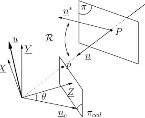
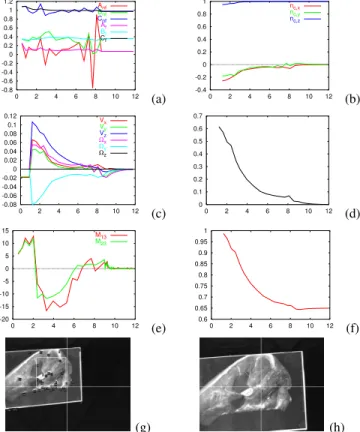
Figure
Documents relatifs
اذلاكو قرلاطلا قولاقح ءارلاكو ليصاحملا عيبك ةصاخلا اهكحمأ نم يتلا تاداريلإا كلذكو اايتما جتان و فقوتلا نكامأ ( 1 ) .ةما لا حلاصملا ض ب 2 ( : للاغتسلاا جوتنم (
In this paper we show how to modify a large class of evolution strategies (ES’s) for unconstrained optimization to rigorously achieve a form of global convergence, meaning
We show that the generating functions of the sequences Av(1234) and Av(12345) correspond, up to simple rational func- tions, to an order-one linear differential operator acting on
In the more classical case of holonomic sequences (satisfying linear recurrences with polynomial coefficients in the index n), fast algorithms exist for the computation of the N
We use the fact that skewness should decay toward zero with the square root of horizon, J( H). Otherwise, the term structure of implied skewness reflects a degree
L’archive ouverte pluridisciplinaire HAL, est destinée au dépôt et à la diffusion de documents scientifiques de niveau recherche, publiés ou non, émanant des
D es rêveries et des jeux d’enfant aux multiples refuges des profes- sionnels de la nature et des loisirs, la liste est longue de toutes les formes d’abris : tentes,
Une étude ethno-vétérinaire des plantes médicinales a été réalisée dans la région Sidi Hadjes, au sud de M‟Sila dans le but d‟établir un catalogue des plantes médicinales
