Globally convergent evolution strategies
Texte intégral
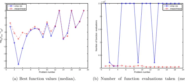
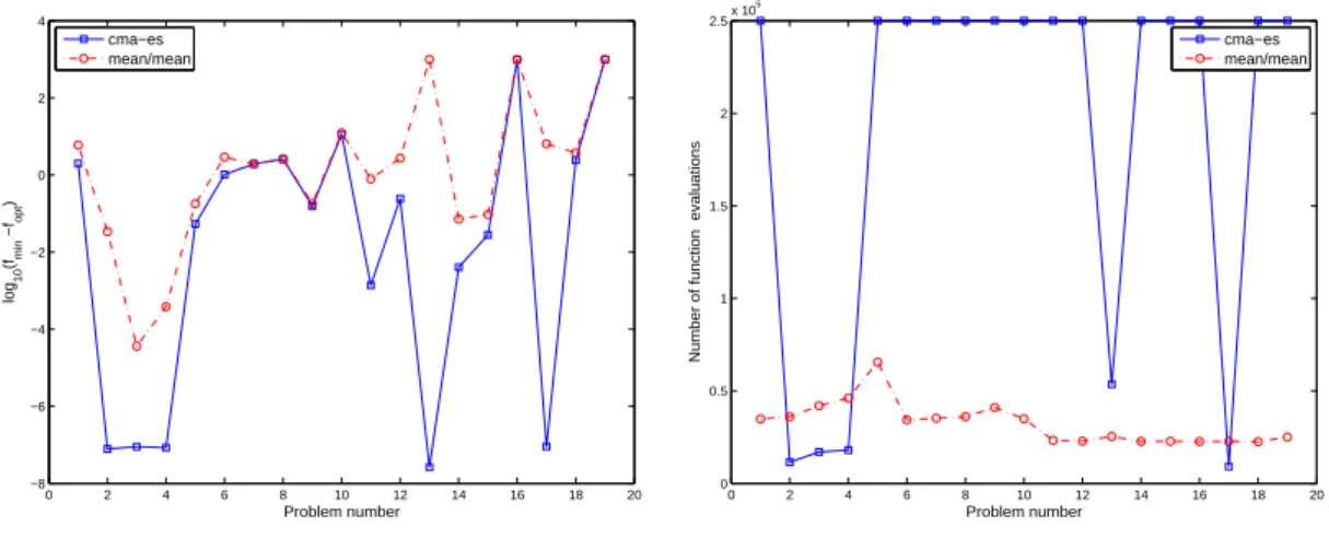
Figure


Documents relatifs
Markov chain theory [18] provides powerful tools to prove linear convergence of randomized algorithms. The general approach consists in finding a class of objective functions for
Considering the “object selected ” to solve a new instance, algorithm scheduling approach defines time slices and running order for each portfolio algorithm and, if a
1- La formulation de la question peut biaiser les réponses. Dans la mesure où la participation du G2 était, à la base, plus élevée, peut-être les élèves
We also show that different covariance matrices for the sampling distribution correspond to a change of norm of the search space, and that this implies that adapting the
In this paper, we establish almost sure linear convergence and a bound on the expected hitting time of an ES, namely the (1 + 1)-ES with (generalized) one- fifth success rule and
Lq wklv sdshu zh vwxg| lq d jlyhq txlwh jhqhudo frpsohwh qdqfldo pdunhw wkh vwdelolw| ri wkh rswlpdo lqyhvwphqw0frqvxpswlrq vwudwhj| dv ghqhg e| Phuwrq +4<:4, zlwk uhvshfw wr
Figure 1: Average marks (the higher the better) of graded assignments and final exam per number of “tutored exercises” sent among the four “tutored exercises” (course in
In this paper we have proven the local convergence of the continuous time model associ- ated to step-size adaptive ESs towards local minima on monotonic C 2 -composite func- tions1.
