Preventive countermeasures for transient stability-constrained power systems

PREVENTIVE COUNTERMEASURES FOR

TRANSIENT STABILITY-CONSTRAINED POWER SYSTEMS

D. Ruiz-Vega, D. Ernst*, C. Bulac, M. Pavella, D. Sobajic **, P. Hirsch **

University of Liège, Sart-Tilman B28, B-4000 Liège, Belgium e-mail address: Mania.Pavella@ulg.ac.be

* Research Fellow, FNRS

** Electric Power Research Institute, Palo Alto, California, USA

Abstract: A general transient stability control technique

is applied to the design of preventive countermeasures consisting of rescheduling generators’ active power. The technique relies on SIME, a hybrid direct – time-domain method; and, like SIME, it preserves the accuracy of time-domain methods and their ability to handle any power system modeling, stability scenario and mode of instability. Its application to generation rescheduling may provide various patterns, able to comply with various operational specifics and strategies, as, for example, congestion management or available transfer capability calculations. The paper suggest how the technique may be shaped to choose automatically rescheduling patterns. A sample of such patterns are illustrated via simulations performed on an EPRI test system.

Keywords: Transient stability constraints; Preventive

control; Dynamic security assessment and control; SIME method.

1 INTRODUCTION

A recently developed technique provides effective tools for on-line transient stability assessment and control. This technique aims at assessing, in a horizon of, say, 30 minutes ahead, whether a power system would be able to withstand all plausible contingencies or, on the

contrary, whether some contingencies would drive it out of step, should they occur. In this latter case, the

technique aims at determining preventive

countermeasures against these “harmful” contingencies. Thus, the technique processes in a sequence two main tasks: one which takes care of contingency FILTering-Ranking and Assessment (FILTRA), the other which performs control, i.e., which determines appropriate countermeasures. More precisely, the FILTRA technique aims at identifying, out of a large list of contingencies1, the “interesting” ones that further investigates in detail and classifies into “harmless”, “potentially harmful” and “harmful”2. Finally, FILTRA assesses the harmful contingencies in terms of margins and critical machines (CMs): a stability margin measures “how far from the stability boundary” the system is driven by the occurrence of a harmful contingency; CMs are the machines which first go out of step and which should be controlled in order to make the system able to withstand this contingency. Margins and CMs are essential to the subsequent design of any control [1,2].

1 _{A contingency is meant to be an important disturbance – or}

succession of events, generally cleared by the system protections.

2 _{A “harmful” contingency is a contingency which would drive the}

On the other hand, the control task determines appropriate countermeasures able to stabilize a system subject to harmful contingencies. The type of countermeasure considered in this paper is machines’ generation (active power). Controlling the system thus consists of assessing the amount of generation decrease3 on CMs necessary to stabilize an otherwise unstable case4; note that, in order to meet the load, this decrease should be compensated by an (almost) equal generation increase on the system non-critical machines (NMs). The resulting countermeasures are determined by an iterative procedure. Ref. [3] proposed such a procedure to stabilize contingencies, considered individually, whereas Ref. [4] adapted this procedure to the simultaneous stabilization of many contingencies. On the other hand, a companion paper points out main differences between closed-loop emergency control and on-line preventive control [5]. In all cases, the iterative procedure shows to be fast and robust, i.e. to converge consistently and reliably after a few iterations.

Actually, the number of possible stabilization patterns may be quite large, depending upon the number of CMs and of contingencies to be stabilized. This paper scans a sample of patterns, and shows that it is possible to determine special purpose patterns capable of meeting specific objectives, whether in vertically organized or in unbundled power systems. The illustrations rely on simulations conducted on the EPRI test system C [6]. The choice of this system was suggested by the large number of existing CMs which thus provide a large variety of possible patterns.

2 BASIC CONTROL PROCEDURE: A SHORT DESCRIPTION

The purpose of this section is to give a general description, mainly on the grounds of physically intuitive considerations rather than systematic developments. Such developments may be found in earlier papers, or in [3,4].

2.1 General principle

The transient stability control considered here relies on the hybrid method called SIME. This method replaces the multi-machine system trajectories by the trajectory of a one-machine infinite bus (OMIB) equivalent, and gets transient stability information about the multi-machine system from the equal-area criterion applied to the OMIB.

3 _{Unless the instability mechanism is of the back-swing type.} 4 _{A stability scenario results from the application of a contingency on}

a case or system under given operating conditions. An “unstable case” or “unstable stability scenario” is a scenario which drives the system to instability. For convenience, we will often use the improper though suggestive term “unstable contingency” rather than “unstable stability scenario”; further “stabilizing a contingency” will be used interchangeably with “stabilizing a stability scenario” and “stabilizing the system”.

Thus, SIME assesses the stability properties of a case in terms of:

• the OMIB stability margin, i.e., the excess of the decelerating over the accelerating area of the OMIB P-δ plane5: acc dec A A − = η (1)

• the multi-machine system CMs, i.e. the machines responsible of the system loss of synchronism.

The above notions are illustrated in Figs 1, describing the stability case of contingency Nr 30 considered in Section 3. Figure 1b displays the multi-swing curves up to the “time to (reach) instability”, tu; this is the time

where the instability is detected by the equal-area criterion. The corresponding OMIB is composed of 38 CMs and 50 (= 88-38) NMs. It is interesting to note that of the 38 CMs, 7 are significantly more advanced than the remaining 31. (See also column 6 of Table 4). On the other hand, Fig. 1a displays the OMIB P-δ representation in terms of Pm and Pe. The normalized

unstable margin, η/M, computed according to the general expression (1), equals –1.21 (rad/s)2.

(a) OMIB equal area criterion (b) Swing curves Fig 1. Principle of SIME’s TSA: illustration on the stability case 30 of

section 3.

2.2 Acronyms and notation

In the above description and throughout the remainder of the paper, the following acronyms and notation are used.

EAC: equal area criterion OMIB: one machine infinite bus TSA: transient stability assessment CM: critical machine

NM: non-critical machine

Aacc (Adec): accelerating (decelerating) area in the P-δ

plane

Pa = Pm-Pe: OMIB accelerating power, excess of its

mechanical power (Pm) over its electrical power (Pe)

M: OMIB inertia coefficient

tu: time to (reach) instability, i.e. time where the EAC

identifies the OMIB instability

5 _{For more details about SIME’s basics, see Ref. [5].}

di: (angular) distance or difference between the critical

machine “i” and the most advanced non-critical machine; in the context of the present paper, di is

measured at tu

η : stability margin

Pc (∆Pc): total active power of the CMs (variation of Pc)

2.3 Control: General principle

Inspection of Fig. 1b suggests that, qualitatively, in order to stabilize the multi-machine (i.e. the real) unstable system, one should manage to “pull the CMs closer” to the NMs. On the other hand, Fig. 1a suggests that a way to stabilize the OMIB equivalent, is to lower the Pm curve so as to decrease the accelerating area and,

at the same time, to increase the decelerating area. Quantitatively, the stabilization will be achieved when

0 ) A A ( ) A A ( ) A A

( dec+∆dec− acc+∆acc = η+∆ dec−∆acc = (2)

. ) A A ( or η = − ∆ dec−∆ acc (3)

Actually, it can be shown that [3]

∑

where P_OMIB denotes the mechanical (active) power of the OMIB, Pci the mechanical (active) power of the i-th

CM, and Pc the total generation power of the CMs.

Obviously, the above considerations yield a suggestion rather than a rigorous calculation. Nevertheless, it provides an initial guess to the following iterative stabilization procedure.

For a given negative (unstable) margin η₀ :

(i) decrease Pc0 by ∆Pc0 to get Pc1 = Pc0 −∆Pc0

(ii) decrease the active power of CMs by ∆Pc0 and

increase by the same amount the active power of the NMs

(iii) perform successively a power flow to compute the new operating conditions and a stability run to compute the corresponding stability margin,

1

η

(iv) perform a linear extra- (or inter-) polation as appropriate to get a first-guess power limit PcLim

(v) compute the new power decrease ∆Pc1 using

PcLim and repeat step (ii) and (iii) using the new

∆Pc1 value, and − −− − if η₂ = 0, stop − −−

− otherwise, adjust as appropriate and continue the process.

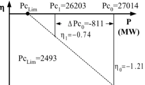
Figure 2 illustrates the first steps of the above procedure in the stability case of contingency 30, whose initial behavior is described in Figs 1.

Fig. 2: First steps of the stabilization procedure applied for case 30 of section 3.

Expression (4) suggests that, whenever there are many CMs, there exist many degrees of freedom as to the distribution of ∆Pc among them. For example, one may think of distributing the active power decrease ∆Pcon: • all CMs proportionally to the product d ∗_i M_i,

where di denotes the (angular) distance of the i-th

CM with respect to the most advanced NM, and Mi

its inertia coefficient;

• (some of) the more advanced CMs;

• all CMs proportionally to their inertia coefficients; • all CMs by the same amount.

Further, instead of stabilizing individually each contingency (i.e., each unstable scenario arising from the application of a harmful contingency), one can stabilize all harmful contingencies simultaneously. One way of doing so has been proposed in Ref. [4]. Another way is used in the next section.

Obviously, the above possibilities may yield a very large number of patterns, of which some are more interesting than some others. Also, some patterns may not be feasible (for example it may not be possible to report the whole decrease on a single CM or on a subset of CMs). However, they suggest that a priori various solutions may be thought of, able to fit various objectives.

Finally, an even larger number of possibilities are left for the power report on NMs, apart maybe from some very specious ones which could destabilize the power system. (For example, think of the case where the total power increase would be reported on the most advanced NM: even if this increase does not impose generation exceeding the machine’s maximum power, it could cause its loss of synchronism.)

Next section focuses on various patterns of power distribution among CMs. The combined rescheduling of CMs and NMs will also be shortly discussed.

3 CONTROL PATTERNS

This section mainly focuses on the CMs’ power rescheduling. The descriptions rely on a concrete example which facilitates explanations; at the same time, it suggests that the number of control patterns may a priori be extremely large.

η ηη η P (MW) Pc₀=27014 Pc₁=26203 η₀= − 1 .2 1 η₁= − 0 .7 4 Pc_Lim ∆ Pc₀=-811 Pc_Lim=2493

3.1 Simulations description

The simulations are performed on the EPRI test system C, having 434 buses, 2357 lines and 88 machines (of which 14 are modeled in detail) [6]. The considered base case has a total generation of 350,749 MW (operating conditions #6).

The SIME package is coupled with the ETMSP program [7].

The contingencies considered are 3-φ short-circuits applied at 500 kV buses and cleared 95 ms after their inception6, generally by opening one line7.

An initial list of 36 contingencies has been screened by FILTRA which finally identified and assessed 4 harmful ones, labeled contingencies 1, 10, 11 and 30.

These harmful contingencies have been stabilized first individually, then simultaneously. In both cases, the stabilization iterative procedure starts with :

• the stability (negative) margin(s) and the corresponding CMs provided at the end of the FILTRA technique, (thus considered to be iteration Nr 0);

• the application of a ∆Pc0 decrease on CMs

corresponding to 3% of their total initial power, Pc0.

3.2 Defining stabilization patterns

The individual stabilization of the four harmful contingencies has been performed using the following control patterns:

• Pattern 1 : the active power decrease ∆Pc is distributed on all CMs proportionally to the product d ∗i Mi;

• Pattern 2 : the active power decrease ∆Pc is distributed equally among the 7 most advanced CMs;

• Pattern 3 : the active power decrease ∆Pc is distributed on all CMs proportionally to their inertia coefficients, Mi;

• Pattern 4 : the active power decrease ∆Pc is equally distributed on all CMs.

On the other hand, the simultaneous stabilization of all four harmful contingencies has been performed according to the procedure described below, in § 3.3.3.

6 _{Note that the contingencies clearing time is slightly different from}

that used in the simulations reported in [5] (100 ms). Further for contingency Nr 1 the line tripped here to clear the fault is different from that in [5].

7 _{Except for the simulations of § 3.3.7 where there are two lines}

tripped.

3.3 Simulation results

The results are gathered in Tables 1 to 4. They are described and commented below.

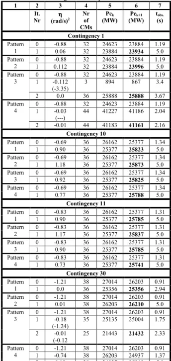
3.3.1 Individual stabilization of cases (Table 1)

Table 1 gives a detailed account of the resulting iterative procedure. It is horizontally subdivided into 4 parts, corresponding to the 4 harmful contingencies, and vertically into the following columns:

• Column 1 : pattern label;

• Column 2 : iteration number; (remember, iteration 0 is the output of the FILTRA software);

• Column 3 : corresponding stability margin, normalized by the OMIB’s inertia coefficient:

2 u 2 1_ω − =

η (rad/s)2, if the case is unstable; • Column 4 : corresponding number of CMs; • Column 5 : total active power generated by the

CMs at iteration k;

• Column 6 : total active power generated by the CMs at iteration (k+1); this power results from either the initial decrease of 3% of the total active power (iteration Nr 0) or the value obtained by linear extra- (inter-)polation of successive margins. For example, Fig. 2 illustrates this extrapolation in the case of contingency 30. It is important to note that the extrapolation procedure must consider the same CMs; the SIME method is adapted to properly handle situations when the CMs’ group change from one simulation to the other. Finally note that the values in bold indicate the total active power of CMs obtained at the end of the iterative procedure. Clearly, the total active power decrease imposed by the stabilization procedure is given by subtracting the final value (in bold) from the initial value, provided that these two values refer to the same CMs.

• Column 7: observation time. For an unstable simulation, this time corresponds to tu, the time

where SIME detects the OMIB instability and stops the time-domain simulation; for a stable simulation, the observation time covers the maximum integration period, in order to guarantee absence of any multi-swing instability (here, 5 seconds). Note that in case multi-swing instabilities are not of concern, this observation time reduces to the time to reach first swing stability (e.g., see in Fig. 3a, the solid line Pe

curve).

3.3.2 Discussion of results of Table 1

From the standpoint of the iterative procedure as such,

the four considered patterns seem equally effective: they converge to an accurate solution generally after one iteration only, even in cases where there is a change of CMs, as in Pattern 3; for this pattern and contingency 1,

the value given between brackets corresponds to the margin of iteration 0 for the 3 machines found to be critical at iteration 1.

From a pragmatic point of view, however, it is quite obvious that Patterns #1, 3 and 4 are impracticable, at least in cases where the number of CMs is large, while Pattern 2 seems more interesting and sound.

It is clear that many other patterns could be thought of, able to modify the generation of some CMs, selected for specific purposes.

3.3.3 Simultaneous stabilization of cases (Table 2)

To stabilize simultaneously contingencies having in common (some) CMs, it seems a priori interesting to focus on the most unstable case(s). Among the various patterns using this observation, the one summarized in Table 2 and shortly commented below takes advantage of the fact that at least 10 CMs are common to all 4 contingencies (actually, there are 32 common CMs).

Table 2: Simultaneous stabilization of the 4 harmful contingencies 1 2 3 4 5 Cont. 1 Cont. 10 Cont. 11 Cont. 30 Iteration 0 η η η η (rad/s)2 _{-0.88 -0.69 -0.83 -1.21} Pc0 24623 26162 26162 27014 Nr of CMs 32 36 36 38 Machine Nr Pcoi 1877 821 1878 769 1873 821 1870 821 1771 779 1855 821 1854 769 1783 220 1871 340 1826 1524 Angle order (gap) 1 (66.5) 2 (66.4) 3 (66.3) 4 (66.3) 5 (63.1) 6 (63.1) 7 (61.2) 8 (46.0) 9 (43.0) 10 (41.6) Angle order (gap) 21 (53.3) 23 (52.9) 22 (52.0) 19 (46.7) 24 (44.8) 2 (44.7) 30 (43.6) 26 (43.3) 18 (42.9) 17 (41.5) Angle order (gap) 19 (52.4) 21 (51.9) 20 (50.9) 18 (47.9) 26 (47.9) 24 (46.6) 30 (46.0) 25 (45.7) 16 (45.4) 15 (44.4) Angle order (gap) 2 (79.4) 1 (79.2) 4 (79.1) 3 (79.1) 5 (74.8) 6 (74.5 7 (74.2) 18 (65.7) 22 (59.6) 36 (53.8) Iteration 1 η η η η (rad/s)2 _{0.218 1.22 0.22 0.01} Pc1 23811 (23973) 25351 (25871) 25351 (25833) 26203 (26210) Nr of CMs 32 36 36 38

Column 1 of the Table 2 lists the 10 more advanced CMs, classified at tu, for contingency 1, as well as the

initial generation of these machines. On the other hand, columns 2 to 5 of the table specify these machines’ classification for the other contingencies, along with their respective angular distance (in degrees), di, from the corresponding most advanced NM.. Note that of these 10 CMs, 7 are top machines for contingencies Nr 1 and 30, which are the severer contingencies among the 4, while for contingencies Nr 10 and 11 these CMs are located rather far away from the top.

The simulations start with a total power decrease ∆Pc=.03*27,014 = 811 MW. (Actually, this is the maximum power decrease, imposed by the severest contingency 30.) Decreasing the initial powers Pc0 of

the 4 contingencies by this ∆Pc yields the Pc1 values

indicated in row 2 of iteration Nr 1. The corresponding new margins are all positive, though for contingency 4 it is almost zero. The Pc values listed between brackets are obtained by interpolating η0 and η1.

3.3.4 Discussion of results of Table 2

Obviously, stabilizing the 4 contingencies simultaneously is as straightforward and (almost) as inexpensive as stabilizing them individually. Of course, contingencies Nr 1, 10 and 11 are slightly over-Table 1: Individual stabilization of the 4 harmful contingencies

using 4 different patterns

1 2 3 4 5 6 7 It. Nr η ηη η (rad/s)2 Nr of CMs Pck (MW) Pck+1 (MW) tobs. (s) Contingency 1 Pattern 1 0 -0.88 32 24623 23884 1.19 1 0.06 32 23884 23934 5.0 Pattern 2 0 -0.88 32 24623 23884 1.19 1 0.112 32 23884 23996 5.0 Pattern 3 0 -0.88 32 24623 23884 1.19 1 -0.112 (-3.35) 3 894 867 3.4 2 0.0 36 25888 25888 3.67 Pattern 4 0 -0.88 32 24623 23884 1.19 1 -0.03 (---) 44 41227 41186 2.04 2 -0.01 44 41183 41161 2.16 Contingency 10 Pattern 1 0 -0.69 36 26162 25377 1.34 1 0.90 36 25377 25823 5.0 Pattern 2 0 -0.69 36 26162 25377 1.34 1 1.18 36 25377 25873 5.0 Pattern 3 0 -0.69 36 26162 25377 1.34 1 0.92 36 25377 25825 5.0 Pattern 4 0 -0.69 36 26162 25377 1.34 1 0.77 36 25377 25788 5.0 Contingency 11 Pattern 1 0 -0.83 36 26162 25377 1.31 1 0.90 36 25377 25785 5.0 Pattern 2 0 -0.83 36 26162 25377 1.31 1 1.17 36 25377 25837 5.0 Pattern 3 0 -0.83 36 26162 25377 1.31 1 0.90 36 25377 25785 5.0 Pattern 4 0 -0.83 36 26162 25377 1.31 1 0.73 36 25377 25741 5.0 Contingency 30 Pattern 1 0 -1.21 38 27014 26203 0.91 1 0.0 36 25356 25356 2.94 Pattern 2 0 -1.21 38 27014 26203 0.91 1 0.01 38 26203 26210 5.0 Pattern 3 0 -1.21 38 27014 26203 0.91 1 -0.18 (-1.24) 35 25135 25004 1.75 2 -0.01 (-0.12 25 21443 21432 2.33 Pattern 4 0 -1.21 38 27014 26203 0.91 1 -0.74 38 26203 24937 1.37 2 0.19 38 24937 25212 5.0

stabilized: in fact, their corresponding Pc values between brackets indicate that the “price” to pay is respectively of 182, 520 and 482 MW. These powers are, however, negligible in terms of percentage of the total power of their CMs.

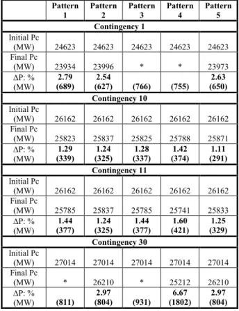
3.3.5 Total power decrease (Table 3)

Table 3 aims at comparing the total power decrease of the 5 patterns, necessary to stabilize the contingencies either individually or simultaneously. This decrease is expressed in MW and in percent of the total initial power of the corresponding CMs. The asterisk suggests that there is a change of CMs between the initial (unstable) and final (stabilized) configuration; hence the difficulty to assess the decrease in percent.

Table 3: Total power decrease of the various patterns. Pattern 1 Pattern 2 Pattern 3 Pattern 4 Pattern 5 Contingency 1 Initial Pc (MW) 24623 24623 24623 24623 24623 Final Pc (MW) 23934 23996 * * 23973 ∆P: % (MW) 2.79 (689) 2.54 (627) (766) (755) 2.63 (650) Contingency 10 Initial Pc (MW) 26162 26162 26162 26162 26162 Final Pc (MW) 25823 25837 25825 25788 25871 ∆P: % (MW) 1.29 (339) 1.24 (325) 1.28 (337) 1.42 (374) 1.11 (291) Contingency 11 Initial Pc (MW) 26162 26162 26162 26162 26162 Final Pc (MW) 25785 25837 25785 25741 25833 ∆P: % (MW) 1.44 (377) 1.24 (325) 1.44 (377) 1.60 (421) 1.25 (329) Contingency 30 Initial Pc (MW) 27014 27014 27014 27014 27014 Final Pc (MW) * 26210 * 25212 26210 ∆P: % (MW) (811) 2.97 (804) (931) 6.67 (1802) 2.97 (804)

3.3.6 Discussion of results of Table 3

Observe that the total power required for the stabilization of the various contingencies is quite similar, except maybe for pattern 4 which appears more expensive in terms of total power decrease on CMs. This is quite normal, since this pattern considers all CMs to be equally important for stabilizing a case, while they are not.

3.3.7 Stabilization of a very unstable case (Table 4)

Table 4 reports on a simulation carried out with contingency Nr 1, with, however, a different clearing scenario than previously: the contingency is cleared by opening two lines (instead of one considered so far). The structure of the table is similar to that of Table 1. Notice that here the asterisk indicates that there is no margin, i.e., no equilibrium position of the system in its

post-fault configuration (see the dotted lines of Fig. 3a: Pe curve does not intersect the Pm curve). In the absence

of stability margin, the asterisk gives the minimum distance (in MW) between the Pm and the Pe curves. The

iterative procedure then starts by extrapolating such distance values, expressed in MW, in order to make the Pe curve intersect the Pm curve. It then continues in the

normal way, previously described.

Table 4: Stabilization of an extremely severe contingency

1 2 3 4 5 6 It. Nr ηη ηη (rad/s)2 Nr of CMs Pck (MW) Pck+1 (MW) tobs. (s) 0 -2591.6* 7 5600 5041 0.330 1 -1966.5* 7 5041 3431 0.380 2 -343.6* 7 3431 2815 0.605 3 -2.898 7 2815 2731 0.935 4 -2.282 7 2731 2423 1.015 5 0.675 7 2423 2493 5.000

Figures 3a and 3b portray the curves obtained in the OMIB P-δ and the phase planes respectively. For the sake of clarity, only two out of the 5 iterations are described; they are represented by the dotted-line and the solid-line curves, corresponding respectively to iterations 0 and 5, i.e., to the most unstable and to the stabilized configurations.

(a) P-δ plane (b) Phase plane

Fig. 3: Two extreme simulations (iterations 0 and 5) of the procedure of §3.3.7.

Dotted lines: Pc0=5600 MW;

Solid lines: Pc5=2423 MW. 3.3.8 Discussion of results of Table 4

Note the robustness of the iterative procedure: it is as accurate as all other cases, even if requiring some more iterations (first with MW margins, second with “normal” (rad/s)2 margins), because of the severity of the instability.

Obviously, stabilizing this extremely severe case requires a significantly more important countermeasure (decrease of active power on CMs) than “normal cases”. From this point of view, the size of the implied countermeasure could be deemed too expensive to be applied preventively.

3.4 General discussion

It is interesting to observe that stabilizing the various contingencies generally implies rather inexpensive countermeasures. Indeed, apart from operating

conditions subject to extremely severe contingencies, these countermeasures imply a small percentage of active power decrease on CMs.

The second observation is that, generally, the number of sound patterns is large enough; this provides many possibilities for the choice of CMs on which to apply the countermeasures, necessary to the system stabilization vis-à-vis harmful contingencies, likely to occur.

The third observation is that a significantly larger number of degrees of freedom is provided for the choice of NMs. Different solutions may therefore be exploited in order to achieve pre-assigned objectives. Reference [4] has proposed the use of an OPF program in order to realize an as large as possible transfer power on a given corridor (cut-set), connecting two areas. The same OPF program could advantageously be used to meet other objectives, such as stability-constrained congestion management. At the same time, the OPF could also meet static constraints.

All in all, it thus appears that: (i) transient stability countermeasures may imply rather negligible power rescheduling, technically easy to realize and affordable from an economic point of view; (ii) the design of such countermeasures is accurate and fast enough to comply with on-line operational requirements; (iii) transient stability constraints may be taken into account together with static constraints via the combined use of SIME and OPF programs.

CONCLUSIONS

This paper has dealt with the design of countermeasures appropriate for on-line preventive transient stability control. The countermeasures rely on active power rescheduling, or, more precisely, on power transfer between critical and non-critical machines. The way of rescheduling power on critical machines relies on SIME, while an OPF program could advantageously take care of power rescheduling on non-critical machines

It was found that in real systems the number of rescheduling patterns on critical machines may be very

large, thus leaving room for specific requirements. On the other hand, the number of rescheduling patterns on non-critical machines is even larger, thus leaving room for meeting operational objectives, such as available transfer capability or congestion management calculations.

The resulting method was thus found to be extremely flexible, and, in addition, robust, accurate and fast enough to comply with on-line operational requirements.

REFERENCES

[1] Ruiz-Vega, D.; Ernst, D.; Machado Ferreira, C.; Pavella, M.; Hirsch, P. and Sobajic, D. “A Contingency Filtering, Ranking and Assessment Technique for On-line Transient Stability Studies”. To be presented at the DRPT2000 conference. London, UK; April 2000.

[2] Ernst, D; Ruiz-Vega, D.; Pavella, M.; Hirsch, P. and Sobajic, D.: “A Unified Approach to Transient Stability Contingency Filtering, Ranking and assessment”. Submitted to the IEEE Trans. on Power Systems.

[3] Ruiz-Vega, D.; Bettiol, A. L.; Ernst, D.; Wehenkel, L. and Pavella, M.: “Transient Stability-Constrained Generation Rescheduling”. Bulk Power System Dynamics and Control IV – Restructuring, Santorini, Greece, August 1998, pp. 105-115. [4] Bettiol, A. L.; Wehenkel L. and Pavella, M.: “Transient

Stability-Constrained Maximum Allowable Transfer”, IEEE Transactions on Power Systems, Vol. 14, No. 2, May 1999, pp.654-659.

[5] Ernst, D; Ruiz-Vega, D. and Pavella, M.: (1999) “Preventive and Emergency Transient Stability Control”. VII Symposium of Specialists in Electric Operational and Expansion Planning, SEPOPE 2000, May 21rd_-26th _{2000, Curitiba Brazil}

[6] “Standard Test Cases for Dynamic Security Assessment”, Final EPRI report No. EPRI TR-105885, Electric Power Research Institute, Project 3103-02 –03, December, 1995.

[7] “Extended Transient Midterm Stability Program Version 3.1 User’s manual” Final EPRI report No. EPRI TR-102004, Electric Power Research Institute, Projects 1208 –11 -12 –13, May, 1994.

Acknowledgements

The first author gratefully acknowledges the financial assistance given by the Consejo Nacional de Ciencia y Tecnología, México for his PhD studies. The financial support of the Electric Power Research Institute (project WO#3103-10) for performing investigations on the EPRI system is thankfully acknowledged