film
J. Brisbois,1, a)B. Raes,2, 3 J. Van de Vondel,2V. V. Moshchalkov,2and A. V. Silhanek1 1)
D´epartement de Physique, Universit´e de Li`ege, B-4000 Sart Tilman, Belgium 2)
INPAC – Institute for Nanoscale Physics and Chemistry, Nanoscale Superconductivity and Magnetism Group, K.U.Leuven, Celestijnenlaan 200D, B–3001 Leuven, Belgium
3)
Current address: Physics and Engineering of Nanodevices, Institut Catal`a de Nanotecnologia (ICN), Campus de la UAB, Edifici ICN2, 08193 Bellaterra, Spain
(Dated: 27 February 2014)
By means of scanning Hall probe microscopy technique we accurately map the magnetic field pattern produced by Meissner screening currents in a thin superconducting Pb stripe. The obtained field profile allows us to quantitatively estimate the Pearl length Λ without the need of pre-calibrating the Hall sensor. This fact contrasts with the information acquired through the spatial field dependence of an individual flux quantum where the scanning height and the magnetic penetration depth combine in a single inseparable parameter. The derived London penetration depth λL coincides with the values previously reported for bulk Pb once the kinetic suppression of the order parameter is properly taken into account.
I. INTRODUCTION
The thermodynamic hallmark of superconductivity is the ability to expel a magnetic field. This phenomenon is produced by macroscopic screening currents circulat-ing at the border of the superconductcirculat-ing material, which in turn generate a magnetic field counteracting the ap-plied one in the interior of the superconductor. In finite size samples, the shielding (or Meissner) currents lead to a reinforcement of the field at the border of the sample usually accounted for through a demagnetization tensor. Since▽ × ⃗B = µ0J , a perfect screening with a discontin-⃗ uous jump in the magnetic field at the sample’s borders, would need unrealistic diverging currents. In reality, fi-nite screening currents run in a thin layer close to the sample’s surface and the field penetrates into the super-conductor over a material dependent distance λ called the magnetic penetration depth. Its determination is of fundamental importance as it is closely related to param-eters relevant for applications, like the lower critical field Hc1 at which penetration of flux quanta becomes ener-getically favourable, or the depairing current density Jdp corresponding to the maximum current that a supercon-ductor can sustain before restoring the normal metallic behavior.
An absolute determination of λ is regarded as a very challenging experimental work. In general, the avail-able techniques can be grouped in two broad categories, namely bulk integrated-response techniques and local probe techniques. Bulk techniques1–6 average the re-sponse of the whole sample and therefore are not sen-sitive to the local details such as possible material in-homogeneities . Local techniques7–12 not only allow one to gain insights at the microscopic level but can be also considered as a more direct way to assess λ . Within the
a)Electronic mail: jbrisbois@ulg.ac.be
local probe category, the most popular approach for es-timating λ consists of mapping the field profile of an iso-lated flux quantum and track its temperature evolution. Unfortunately, irrespective of whether the flux quantum is an Abrikosov vortex present in a thick sample, or a Pearl vortex13 characteristic of thin films, the vertical component of the magnetic field picked up by the sensor depends on a single variable, z0+λ, forming an indis-sociable additive combination of the vertical separation between the sensor and the surface of the superconduc-tor, z0, and λ. Therefore, the precision of the extracted λ is directly linked to the quality of the calibration of the z-positioners and relies on perfect knowledge of the geometrical configuration and the sensor mounting.
In this study, we propose an alternative method to determine the penetration depth λ which has not been explored so far and does not require pre-calibration pro-cedures of the magnetic sensor. Its precision depends on the good knowledge of the sample geometry. The ap-proach consists of mapping the magnetic field profile at the border of the sample produced by Meissner screen-ing currents. In contrast to the centrosymmetric field landscape of an isolated vortex, now the contribution of the vertical separation z0and the penetration depth con-tribute separately to the vertical component of the de-tected magnetic field, thus facilitating the estimation of λ. Even though the method is illustrated with a par-ticular magnetic probe (i.e. a Hall sensor), it is appli-cable to any other scanning magnetic probe techniques such as magnetic force microscopy (MFM) or SQUID microscopy. In addition, this method can also work for current-driven transport bridges at zero external field.
II. EXPERIMENTAL DETAILS
We study the response of a Pb strip of length L = 3 mm, width 2a = 600 µm and thickness t = 50 nm de-posited on an insulating SiO2/Si substrate. The surface
is protected by a 60 nm thick insulating Ge layer to pre-vent oxidation. The sample is patterned with a square lattice of square holes of side length b = 600 nm and period w = 3 µm, as schematically shown in Fig. 1. As we discuss below, the ratio b/w has been chosen in such a way that the holes have negligible effect on the penetration length while allowing us to readily check the onset of flux penetration into the sample, i.e. the limit of the Meissner state. A superconducting critical tem-perature Tc= 7.2 K was determined by ac-susceptibility measurements14. A 50 nm thick gold layer covers the sample to allow using a tunneling conducting tip as a feedback loop to approach the sample surface.
FIG. 1. Sketch of the nanostructured thin superconducting Pb film of thickness t = 50 nm. The film has a length L and a width 2a and it is patterned by a square lattice (period w) of square holes (side-length b). In the Meissner state, when a constant magnetic field Bappis applied, screening currents ⃗j(u) flow in the sample. Each infinitesimal element du centred
on u generates a contribution d ⃗Bindto the magnetic field ⃗Bind.
The total field is calculated by Biot-Savart’s law and is the sum of ⃗Bappand the contribution of the screening currents.
The Hall probe is a cross-shaped 2DEG
(GaAs/AlGaAs) scanning alongside the sample surface, fed with a constant dc current∼ 20µA and with readout voltage proportional to the component of the magnetic field perpendicular to the probe. Scanning Hall probe microscopy (SHPM) exhibits several advantages for our experiment : it is non invasive, it offers a good compro-mise between spatial and field resolution15 and, in lift mode, it is a relatively fast way to get two-dimensional images of the magnetic field. We use a commercial low-temperature SHPM (NanoMagnetics Instruments) modified by adding a piezoelectric horizontal slider to allow the adjustment of the sample position. The vertical position is adjusted by a piezoelectric slider (coarse positioning of step p∼ 0.8 µm according to the specifications of the manufacturer) and a piezoelectric tube (fine positioning).
A standard approaching process16ends when a tunnel current of 0.5 nA is obtained, corresponding to a tunnel resistance of 200 MΩ and a tip-sample distance smaller than 1 nm. Once the tip is in STM-contact with the sample, the ultimate lower limit for the height above the
sample surface is determined by the depth of the 2DEG below the surface of the heterostructure, typically 100 nm. However, an additional and far more important lim-itation comes from the angle between the sample and probe chip∼ 1 − 2◦ and the fact that the Hall sensor is about 15 µm away from the STM tip as schematically shown in Fig. 2. The distance between the active area and the STM tip combined with the tilt angle contributes to the height of the probe. In principle it is possible to scan the sensor over the sample surface while keeping the tunneling current constant using a PID protocol on the z-piezo, obtaining simultaneously the topography and the magnetic field distribution. In this configuration, the Hall sensor scans over the sample surface at a minimum distance of 600 nm. However, in practice we lift the scan head a few hundreds of nm after STM-contact at the highest corner of the scan area, and the scan is performed at this fixed distance z0 ∼ 1 µm. The lift height is lim-ited by the surface roughness within the scan area and can be continuously adjusted during scanning in both lat-eral and transversal directions for compensating the tilt of the sample. This lift-mode allows for faster imaging, with less risk of crashing the probe. In this work, keep-ing in mind the aforementioned restrictions, we introduce a protocol to precisely determine the height of the Hall sensor z0. Moreover, this characterization allows us to obtain a good estimate for λL.
FIG. 2. Schematic illustration of the sample-sensor chip ori-entation and position. In this configuration, the STM tip is always the point of the Hall sensor closest to the sample, thus limiting the risk of crashing the probe during the approach. The minimal distance z0is limited by the depth of the 2DEG
in the heterostructure and by the distance between the STM tip and the Hall cross. Moreover, the sensor is usually lifted by a few hundreds of nm to allow fast imaging.
III. FIELD PROFILE PRODUCED BY MEISSNER CURRENTS
A. Theoretical Model
Let us start analyzing the magnetic response of a su-perconducting strip in the Meissner state as shown in Fig. 1. The strip occupies the space|x| ≤ a, |y| ≤ L/2 ≫ a and |z| ≤ t/2 ≪ a. After cooling down the sample be-low Tc, a constant magnetic field Happ = Bapp/µ0 is applied perpendicularly to the surface (zero-field cooling process). Consequently, screening currents flow around the strip in an attempt to shield Happ inside the super-conductor. Assuming that t < λ, the current density is nearly independent of z across the film thickness, and therefore it is convenient to consider only the surface current density ⃗JS(x, y) defined by averaging the volume current density ⃗j(x, y, z) over the thickness of the strip:
⃗
JS(x, y) = ∫ t/2
−t/2⃗j(x, y, z)dz.
(1)
The total magnetic field ⃗Btot(x, y, z) at the point of coordinates (x, y, z) is the sum of two contributions : the applied field ⃗Bapp and the field generated by the screen-ing currents ⃗Bind(x, y, z). As L ≫ a, t, ⃗Btot and ⃗JS do not depend on y. In what follows, the only component of ⃗Btot(x, z) considered relevant for measurements with magnetic probes is the z-component Bz(x, z). We can work out an expression for ⃗Bind(x, z) based on the nota-tions of Fig. 1.
The field d ⃗Bindproduced by an infinitesimal portion of material du crossed by a current I(u) can be determined by Amp`ere’s law and, by subsequently summing up the contribution of each infinitesimal portion du we obtain,
Bind,z(x, z) = µ0 2π ∫ a −a (x− u)JL(u)du (x− u)2+ z2 , (2) where JLis the linear current density defined as JL(x) = JS(x, y)dy. The z-component of ⃗Btot at (x, y, z) is thus given by Bz(x, z) = µ0 2π ∫ a −a (x− u)JL(u)du (x− u)2+ z2 + Bapp. (3) An expression for JL(u) obtained from the London-Maxwell equations for a thin (t≪ a) rectangular strip is given by Plourde et al.17 for a constant magnetic field perpendicular to the surface. When a/Λ ≫ 1 where Λ = λ2/t is the Pearl length, J
L(u) is expressed as
JL(u) = 2uBapp
µ0 √
(a2− u2) +4a
πΛ
. (4)
By inserting this relationship in Eq. (3) we can deduce the relative change of magnetic field as the Hall probe
scans the width of the strip at a height z: Bz(x, z) Bapp = 1 + 1 π ∫ a −a (x− u)udu ((x− u)2+ z2)√(a2− u2) +4a πΛ . (5) In the next section, we will use this equation to model the Bz(x,z) profiles obtained experimentally at different distances z from the surface of the superconductor.
B. Experimental results
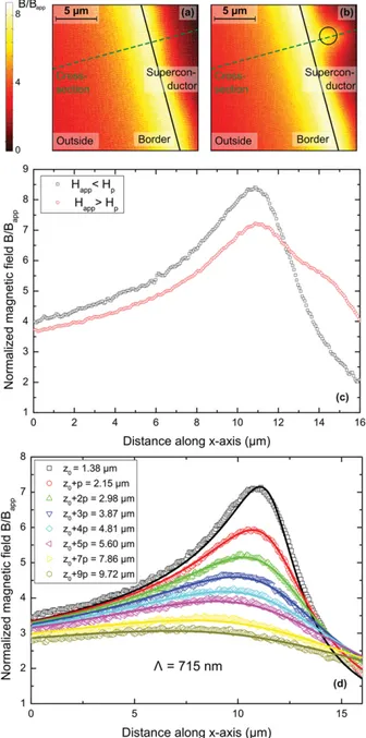
In order to obtain the magnetic field profile in the Meissner state, a series of SHPM images were recorded at the border of the Pb strip at T = 4.2 K and Happ = Bapp/µ0 in zero field cooling. An example of the result-ing field landscape is shown in Fig. 3(a). The border of the strip can easily be localized by the bright strip cor-responding to the magnetic field generated by the Meiss-ner screening currents. For each image we averaged ten cross-sections taken perpendicularly to the border in or-der to reduce the noise-to-signal ratio of the field profiles. We then divide the result by Bapp and fit the results fol-lowing Eq. (5). This equation indicates that the larger the applied field, the bigger will be the signal detected and therefore higher signal-to-noise ratio can be achieved. This argument holds for fields below certain threshold Hp at which flux quanta penetrates into the sample14. Since the holes act as pinning centers preventing vortices to proceed towards the middle of the sample, the pinned vortices contribute to the field measured at the border of the sample and serve as an indication that the condi-tion Happ > Hp has been achieved. This is illustrated in Fig. 3(b) where a vortex is indicated by a black cir-cle. In Fig. 3(c) we show the field profile for Happ. Hp and Happ & Hp. Notice that the penetration of a flux quantum relaxes the magnetic field at the border of the sample.
Once the value of Hphas been identified, Eq. (5) can be used to model the field profiles at different heights z obtained for Happ . Hp. The experimental data is plot-ted on Fig. 3(d). As z increases, the Bz(x) peak due to the demagnetizing effects broadens and in the limit of z → ∞, it should be recovered Bz(x) = Bapp. The asymmetric shape of the field profile at the border of the sample reflects the long range perturbation of the magnetic field outside the sample, caused by demagneti-zation effect at the border of the strip, which contrasts with a much sharper decay of the magnetic field upon entering the superconductor. More quantitatively, the magnetic field outside (inside) decreases halfway towards its final value Bz= Bapp(Bz= 0) at a distance∼ 7.5 µm (∼ 3 µm) from the border.
The fitting of the curves is based on Eq. (5) for a = 300 µm. All the curves are adjusted simultaneously with the respective scanning heights zi and a common value for Λ as free parameters. The best fitting is ob-tained for Λ = 715± 300 nm and a lowest scanning
FIG. 3. (a) and (b) show the SHPM images of the supercon-ducting strip border in the Meissner state in a constant mag-netic field Happ respectively lower and slightly higher than Hp, the field corresponding to the first vortex entry in the
sample. The bright area indicates the higher magnetic field and is due to the presence of demagnetizing effects at the bor-der of the sample (black line). In panel (b), a vortex trapped by an antidot close to the sample border has been highlighted with a circle. The cross-sections shown in (c) where taken along the green lines. (d) Influence of the distance z be-tween the Hall probe and the sample surface on the normal-ized magnetic field profile at the border of the strip. z0is the
minimum scanning height and p is the stepsize of the vertical piezo slider. The curves computed numerically (continuous lines) from the relation (5) are superposed to the data. In addition to the scanning heights, the model yields a value for the transversal penetration depth Λ = 715± 300 nm.
height z0 = 1.38± 0.15 µm. The resulting profiles are represented on Fig. 3(d) as continuous lines along with the corresponding values for zi. The modelled magnetic field profile evolution with z is in good agreement with the experiment and the estimated value for the step of the vertical slider is around 0.9 µm, close to the expected value of p = 0.8 µm provided by the manufacturer for T = 4.2 K.
Knowing that Λ = λ2/t = 715 nm we can estimate λ(T = 4.2K)≈ 189 nm, and assuming Ginzburg-Landau temperature dependence λ(T ) = λ(0)/√1− T/Tcwe de-duce λ(0)≈ 122 nm. From the temperature dependence of the upper critical field we can estimate a coherence length ξ(0)≈ 33 nm ≪ ξ0= 82 nm meaning that our Pb film falls in the dirty limit. Using the dirty limit correc-tion for the penetracorrec-tion depth λ = (0.64√ξ0/ℓ)−1λLand coherence length ξ(0) = 0.855√ξ0ℓ, it is easy to show that λL ≈ 1.83ξ(0)λ(0)/ξ0 ∼ 89 nm. The fact that we have chosen to work at a field very close to the pen-etration field Hp, implies that the screening current is very close to the depairing current14. It is worth noting that London and Ginzburg-Landau theories give simi-lar results, except at the border of the sample when Happ is close to Hp, which are the conditions of this experiment18. Under these circumstances, it is impera-tive to consider the kinetic suppression of the order pa-rameter ignored within the London approximation but properly accounted in the Ginzburg-Landau formalism. This depletion of the superconducting condensate at the border of the sample leads to a less efficient screening manifested by a larger penetration depth λedge= 1.84λL. This factor results from the decrease of the density of states with increasing current and is described within the first Ginzburg-Landau equation, which expresses conser-vation of energy and effectively couples the Cooper pair-density with the pair velocity19. When taking into ac-count this correction we obtain λL = 48± 11 nm, which is in reasonable agreement with λL = 40 nm obtained by alternative techniques20. Notice that following a sim-ilar analysis and assuming that λLis known, the effective coherence length could be deduced from Λ.
C. Effect of finite size of the sensor
Eq. (5) presumes an infinitely small magnetic sensor and therefore ignores the finite size s of the active area of the Hall probe. Taking into account this effects results in a convolution effect on the real magnetic field. In other words, instead of measuring Bz(x, z), the measured field is given by
⟨B⟩ = ∫
S
dA G(x, y)B(x, y), (6) where S is the active surface and G is the response func-tion accounting for the inhomogeneity of the sensitivity. Several references can be found that calculate G depend-ing on the kinetics of the electrons (diffusive regime21,22,
ballistic regime23,24) and the size of the Hall probe. It is shown that when the Hall sensor operates in the ballistic regime and at low field, the response function can be con-sidered as a constant within the main junction area, with rapid decaying tails in the contact paths and independent of the shape and position of the field inhomogeneity pro-file in the junction. Practically, the convolution product is computed numerically by averaging the field amplitude over the number of neighbouring pixels corresponding to s.
FIG. 4. Influence of the size s of the active area of the Hall probe on the magnetic field profile. The fixed parameters are Λ = 1.2 µm, a = 300 µm and s = 1 µm. The influence of convolution is only visible for the peak and at low z. For values of z & 1 µm used in our experiment, convolution is negligible.
The effect of convolution by the size s of the active area of the Hall probe is visible on Fig. 4. The value of s = 1 µm is deliberately bigger than the real chip value (around 300 nm) to emphasize the effects of convolution. These effects are important only where the field varies quickly as a function of x, i.e. near the peak. For a height z = 0.4 µm significantly lower than the height at which the measurements where taken, the convolution decreases the amplitude of the peak by 6.1% compared to its initial value. For z = 2.0 µm, the influence of convolution is slender and the relative variation of the peak amplitude is of 0.4% . By fixing s = 450 nm, the convolution for z = 2 µm is responsible for a relative amplitude variation of the peak smaller than 0.1%. We can thus safely neglect the influence of the Hall probe size s and the effect of convolution by the active area for our data.
IV. ISOLATED FLUX QUANTUM
Let us now investigate the profile of an individual iso-lated vortex. To that end, we applied a magnetic field Happ ≪ H1 perpendicular to the sample surface, where H1= Φ0/w2is the first matching field at which the
den-sity of vortices coincides with the denden-sity of antidots. In this case, after cooling down the sample to 4.2 K (field-cooling process), the vortices will be separated by a dis-tance much larger than Λ. Thus, we can consider them as isolated, as shown on Fig. 5(a) for the minimal scanning height z0. In order to extract the magnetic field profile from the isolated vortex, we consider the points located on the circumference of circles centred on the vortex and of radius r. We then average the values of the field at these points for r between 0 and 4 µm. We collected sev-eral SHPM images Bz(x, y), at different scanheights z.
FIG. 5. (a) SHPM image at the middle of the superconduct-ing strip after field coolsuperconduct-ing in a constant magnetic field. Two well separated vortices can be seen (bright spots). The values of the field were averaged on circles like the one shown on the figure. The dashed line shows the extension of the ob-tained field profile. (b) Evolution of the magnetic field profile of a single vortex as a function of the height z of the probe. The plain curves represent the fitting based on the magnetic monopole model. This model yields values for L = z + λeff
for different z that are consistent with the expected increase of z between the curves.
Theoretically the field profile of a single vortex line can be described as the field produced by a magnetic monopole25. This model is derived from the bound-ary condition at the superconducting-vacuum interface, where the London equations and the Maxwell equations must be satisfied respectively inside and outside the su-perconductor. It is valid for an infinite plane film with an arbitrary thickness. In the limit of √r2+ z2 ≫ Λ,
where r is the in-plane distance measured from the cen-ter of the vortex and z is the height measured from the surface, the magnetic field profile is described by the fol-lowing expression : Bz(r, z) = Φ0 2π z + λeff (r2+ (z + λ eff)2)3/2 . (7)
where λeff = λ coth(d/2λ). This equation represents the magnetic field of a magnetic monopole of amplitude 2Φ0 localized at a distance λeff beneath the surface. We can consider the vortex as a monopole because the magnetic field is the same as if the flux lines where produced at one single point, and they do not close on themselves26. We use Eq. (7), where Φ0/2π is replaced by a multiplicative constant, to represent the data. The fitting is done for all curves simultaneously with respect to this common constant and the values of zi+ λeff for each curve, which are listed on Fig. 5(b). We can estimate the step p of the vertical slider by comparing the values for the first and the last curves. This yields p = 0.88 µm. It confirms the value of p = 0.9 µm found in the Meissner state and agrees with the theoretical value of 0.8 µm given by the SHPM manufacturer.
From the fitting, we conclude that the magnetic monopole model correctly describes the magnetic field profile of an isolated vortex in a sample with a peri-odic array of holes. Unfortunately, we do not have ac-cess to the probe height z and to λeff separately, be-cause these two parameters appear only through their sum in the theoretical relation. Thus, it is impossible to distinguish between a change in z or λeff, as the effect on the magnetic field is the same. However, assuming λeff = Λ = 715 nm as found in the Meissner state27, we can extract the effective scanning heights zi and we find namely z0 = 0.98± 0.3 µm. This value is smaller than z0 = 1.38 µm found at the border of the sample in the Meissner state.
As we already anticipated in the Experimental section, the value of z0 depends on the location where the scan-ning takes place, since the presence of defects and asperi-ties at the surface of the sample can give different offsets. Actually, atomic force microscopy images in our sample reveal the presence of about 300 nm thick resist leftovers at the border of the sample which are absent in the cen-tre. This resist seems to be source of the discrepancy in our measurements of z0for these two locations.
V. CONCLUSION
In this study, we used SHPM to image the magnetic field landscape at the border of a Pb thin film. Mea-surements of the magnetic field in the Meissner state fol-low the spatial dependency proposed by Plourde et al.17 based on London-Maxwell equations. A procedure is pro-posed which uses the theoretical fitting of these curves to determine the magnetic penetration depth and the probe-sample distance. By taking into account the temperature
dependence of the penetration depth and the kinetic de-pletion of the order parameter we obtained λL = 48± 11 nm, which agrees well with values reported in literature for Pb. We deduced that the separation between the Hall sensor and the sample surface is normally slightly larger than 1 µm and we demonstrated that for these heights, the size of the Hall probe does not introduce significant corrections. In addition, we showed that the magnetic monopole model is appropriate to describe the field pro-file of a single vortex and we used the value of Λ found in the Meissner state to extract the effective scanning height, a crucial parameter needed for obtaining quanti-tative values of the magnetic field.
VI. ACKNOWLEDGEMENTS
This work was partially supported by the Fonds de la Recherche Scientique - FNRS, the Methusalem Fund-ing of the Flemish Government, the Fund for Scien-tic Research-Flanders (FWO-Vlaanderen) and the ARC grant 13/18-08 for Concerted Research Actions, financed by the Wallonia-Brussels Federation. J.B. acknowl-edges support from FRS-FNRS (Research Fellowship). J. V.d.V. acknowledges support from FWO-Vl. The work of A.V.S. is partially supported by ”Cr´edit de d´emarrage”, U.Lg.
1R. Prozorov, R. W. Giannetta, A. Carrington, P. Fournier, R. L.
Greene, P. Guptasarma, D. G. Hinks, and A. R. Banks, Appl. Phys. Lett. 77, 4202 (2000).
2M. Abdel-Hafiez, J. Ge, A. N. Vasiliev, D. A. Chareev, J. Van de
Vondel, V. V. Moshchalkov, A. V. Silhanek, Phys. Rev. B (2013).
3A. T. Fiory, A. F. Hebard, P. M. Mankiewich, and R. E. Howard,
Appl. Phys. Lett. 52, 2165 (1988).
4J. Mao, D. H. Wu, J. L. Peng, R. L. Greene, and S. M. Anlage,
Phys. Rev. B 51, 3316 (1995).
5D. N. Basov, R. Liang, D. A. Bonn, W. N. Hardy, B. Dabrowski,
M. Quijada, D. B. Tanner, J. P. Rice, D. M. Ginsberg, and T. Timusk, Phys. Rev. Lett. 74, 598 (1995).
6J. E. Sonier, R. F. Kiefl, J. H. Brewer, D. A. Bonn, J. F. Carolan,
K. H. Chow, P. Dosanjh, W. N. Hardy, Ruixing Liang, W. A. MacFarlane, P. Mendels, G. D. Morris, T. M. Riseman, and J. W. Schneider, Phys. Rev. Lett. 72, 744 (1994).
7L. Luan, O. M. Auslaender, T. M. Lippman, C. W. Hicks, B.
Kalisky, J.-H. Chu, J. G. Analytis, I. R. Fisher, J. R. Kirtley and K. A. Moler, Phys. Rev. B 81, 100501 (2010).
8L. Luan, T. M. Lippman, C. W. Hicks, J. A. Bert, O. A.
Aus-laender, J.-H. Chu, J. G. Analytis, I. R. Fisher and K. A. Moler, Phys. Rev. Lett. 106, 67001 (2010).
9J. Kim, N. Haberkorn, S.-Z. Lin, L. Civale, E. Nazaretski, B. H.
Moeckly, C. S. Yung, J. D. Thompson and R. Movshovich, Phys. Rev. B 86, 24501 (2012).
10J. Kim, L. Civale, E. Nazaretski, N. Haberkorn, F. Ronning, A.
S. Sefat, T. Tajima, B. H. Moeckly, J. D. Thompson and R. Movshovich, Supercond. Sci. Technol. 25, 112001 (2012).
11A. Kohen, T. Proslier, T. Cren, Y. Noat, W. Sacks, H. Berger
and D. Roditchev, Phys. Rev. Lett. 97, 27001 (2006).
12J. R. Kirtley, C. C. Tsuei, F. Tafuri, P. G. Medaglia, P. Orgiani
and G. Balestrino, Supercond. Sci. Technol.17 217 (2004)
13J. Pearl, Appl. Phys. Lett. 5, 65 (1964)
14J. Gutierrez, B. Raes, J. Van de Vondel, A. V. Silhanek, R. B. G.
Kramer, G. W. Ataklti, and V. V. Moshchalkov Physical Review B 88, 184504 (2013).
16B. Raes, Ph.D. thesis, Catholic University of Leuven, pp. 186,
2013.
17B. L. T. Plourde, D. J. Van Harlingen, D. Y. Vodolazov, R.
Besseling, M. B. S. Hesselberth and P. H. Kes, Phys. Rev. B 64, 14503 (2001)
18D. Yu. Vodolazov, I. L. Maksimov, Physica C 349, 125 (2001). 19K. Fossheim and A. Sudbø, Superconductivity: Physics and
Ap-plications, John Wiley & Sons, p. 234 (2005).
20M. P. Nutley, A. T. Boothroyd, C. Staddon, D. M. Paul and J.
Penfold, Phys. Rev. B 49, 15789 (1994).
21S. Bending and A. Oral, J. Appl. Phys., 81, 3721 (1987).
22Y. G. Cornelissens and F. M. Peeters, J. Appl. Phys., 92, 2006
(2002).
23F. M. Peeters and X. Q. Li, Appl. Phys. Lett. 72, 572 (1998) 24A. K. Geim, S. J. Bending, I. V. Grigorieva, and M. G. Blamire,
Phys. Rev. B 49, 5749 (1994).
25A. M. Chang et al., Appl. Phys. Lett. 61, 1974 (1992) 26G. Carneiro and E. H. Brandt, Phys. Rev. B 61, 6370 (2000) 27In this approximation we are neglecting the fact that the vortex
is trapped in a hole and therefore λ should increase by half the size of the hole. This effect will lead to an even smaller z0. 28A.I. Buzdin, Phys. Rev. B 47, 11416 (1993).
29A.Wahl, V. Hardy, J. Provost, Ch. Simon and A. Buzdin, Physica