James Kilner,
Gareth Barnes,
Robert Oostenveld,
Jean Daunizeau,
Guillaume Flandin,
Will Penny,
1and Karl Friston
11The Wellcome Trust Centre for Neuroimaging, UCL Institute of Neurology, Queen Square, London WC1N 3BG, UK
2INSERM U1028, CNRS UMR5292, Lyon Neuroscience Research Centre, Brain Dynamics and Cognition Team, Lyon, F-69500, France 3Max Planck Institute for Human Cognitive and Brain Sciences, 04303 Leipzig, Germany
4Cyclotron Research Centre, University of Li`ege, 4000 Li`ege, Belgium 5MRC Cognition and Brain Sciences Unit, Cambridge CB2 7EF, UK
6Donders Institute for Brain, Cognition, and Behaviour, Radboud University Nijmegen, 6500 HB Nijmegen, The Netherlands
Correspondence should be addressed to Vladimir Litvak,[email protected] Received 24 September 2010; Accepted 7 December 2010
Academic Editor: Sylvain Baillet
Copyright © 2011 Vladimir Litvak et al. This is an open access article distributed under the Creative Commons Attribution License, which permits unrestricted use, distribution, and reproduction in any medium, provided the original work is properly cited.
SPM is a free and open source software written in MATLAB (The MathWorks, Inc.). In addition to standard M/EEG preprocessing, we presently offer three main analysis tools: (i) statistical analysis of scalp-maps, time-frequency images, and volumetric 3D source reconstruction images based on the general linear model, with correction for multiple comparisons using random field theory; (ii) Bayesian M/EEG source reconstruction, including support for group studies, simultaneous EEG and MEG, and fMRI priors; (iii) dynamic causal modelling (DCM), an approach combining neural modelling with data analysis for which there are several variants dealing with evoked responses, steady state responses (power spectra and cross-spectra), induced responses, and phase coupling. SPM8 is integrated with the FieldTrip toolbox , making it possible for users to combine a variety of standard analysis methods with new schemes implemented in SPM and build custom analysis tools using powerful graphical user interface (GUI) and batching tools.
1. Introduction
Statistical parametric mapping (SPM) is a free and open source academic software distributed under GNU General Public License. The aim of SPM is to communicate and disseminate methods for neuroimaging data analysis to the scientific community that have been developed by the SPM coauthors associated with the Wellcome Trust Centre for Neuroimaging, UCL Institute of Neurology.
The origins of SPM software go back to 1990, when SPM was first formulated for the statistical analysis of positron
emission tomography (PET) data [1,2]. The software
incor-porated several important theoretical advances, such as the use of general linear model (GLM) to describe, in a generic way, a variety of experimental designs [3] and random field theory (RFT) to solve the problem of multiple comparisons arising from the application of mass univariate tests to
images with multiple voxels [4]. As functional magnetic resonance imaging (fMRI) gained popularity later in the decade, SPM was further developed to support this new imaging modality, introducing the notion of a hemodynamic response function and associated convolution models for serially correlated time series. This formulation became an established standard in the field and most other free and commercial packages for fMRI analysis implement variants of it. In parallel, increasingly more sophisticated tools for registration, spatial normalization, and segmentation of functional and structural images were developed [5]. In addition to finessing fMRI and PET analyses, these methods made it possible to apply SPM to structural MRIs [6], which became the field of voxel-based morphometry (VBM).
The first decade of the 21st century brought about two further key theoretical developments for SPM: increasing
use of Bayesian methods (e.g., posterior probability mapping [7]) and a focus on methods for studying functional inte-gration rather than specialization. Dynamic causal modelling (DCM [8]) was introduced as a generic method for studying functional integration in neural systems. This approach uses Bayesian methods for fitting dynamic models (formulated as
systems of differential equations) to functional imaging data,
making inferences about model parameters and performing model comparison. Bayesian model comparison uses an approximation to the model evidence (probability of the data given the model). Model evidence quantifies the properties of a good model; that is, that it explains the data as accurately as possible and, at the same time, has minimal complexity [9–11]. Further development and refinement of DCM and related methods are likely to remain the focus of research in the future.
In the second half of the decade, the research focus of the SPM group shifted towards the analysis of MEG and EEG (M/EEG). This resulted in three main developments. First, the “classical” SPM approach was extended to the analysis of M/EEG scalp maps [12–14] and time-frequency images [15]. Second, a new approach to electromagnetic source reconstruction was introduced based on Bayesian inversion of hierarchical Gaussian process models [16–18]. The Bayesian perspective was also applied to the problem of equivalent current dipole modelling [19]. Third, DCM was extended to M/EEG data and several variants of the approach were validated, focusing on evoked responses [20], induced responses [21], steady state responses [22], and phase coupling [23]. In order to make it possible for our colleagues to apply these methods easily to their data, infrastructure for conversion and pre-processing of M/EEG data from a wide range of recording systems were incorporated in the SPM software, with notable contribution from the developers of the FieldTrip software (http://www.ru.nl/donders/fieldtrip, see Oostenveld et al. in this issue). SPM for M/EEG is con-structed to support the high-level functionality developed by our group and is not intended as a generic repository of useful methods. This distinguishes SPM from some other toolboxes (e.g., FieldTrip).
The present paper focuses on the implementation of these tools in the most recent SPM version, SPM8. We will not rehearse all the technical details of the methods, for which the reader is referred to the relevant papers. Moreover, we will also avoid focusing on specific interface details, as these often change with intensive SPM development. The details we do mention are correct for SPM8 version 4010, released on July 21, 2010. Our aim is to provide an overview of SPM functionality and the data analysis pathways that the software presently supports. This overview is quite long and inclusive. This reflects the fact that the software covers three distinct domains, source reconstruction, statistical parametric mapping (topological inference over various spaces) and dynamic causal modeling. Each entails a set of assumptions and procedures, some of which are fairly basic and common to most analyses of electromagnetic data and some of which are unique to the applications we consider. We have elected to cover all the basic issues for completeness and to relate them to the specific issues within
each domain. However, the readers who are familiar with the basic parts could easily skip these sections. The paper is organized as follows. After presenting a brief overview of the SPM8 user interface, we focus on each of the three core parts of SPM for M/EEG presented above: (i) statistical analysis of images, (ii) Bayesian source reconstruction, and (iii) DCM for M/EEG. The Appendix describes the M/EEG pre-processing infrastructure in SPM8 and explains how to get from raw M/EEG data to the format suitable for analysis with one of the core SPM methods.
2. SPM8 Interface and Overview
The SPM software consists of a library of MATLAB M-files and a small number of C-M-files, using the MATLAB MEX gateway for the most computer-intensive operations. Its installation simply consists of unpacking a ZIP archive on the user computer and adding the root SPM directory to the MATLAB path. More details on the installation (especially compilation of the MEX files if needed) can be found on the SPM wiki on Wikibooks (http://en.wikibooks.org/wiki/ SPM). SPM requires a prior installation of MATLAB, a com-mercial high-end numerical software platform developed by the MathWorks, Inc. (Natick, USA). More specifically, SPM requires version R14SP3 (released in 2005) or any more recent version (up to the latest R2010b). It runs on any platform supported by MATLAB, that is, Microsoft Windows, Macintosh OS, and Linux, 32- and 64-bit. A standalone version of SPM8, compiled using the MATLAB compiler, is available upon request—it allows using most of the SPM functionalities without requiring the availability of a MATLAB licence.
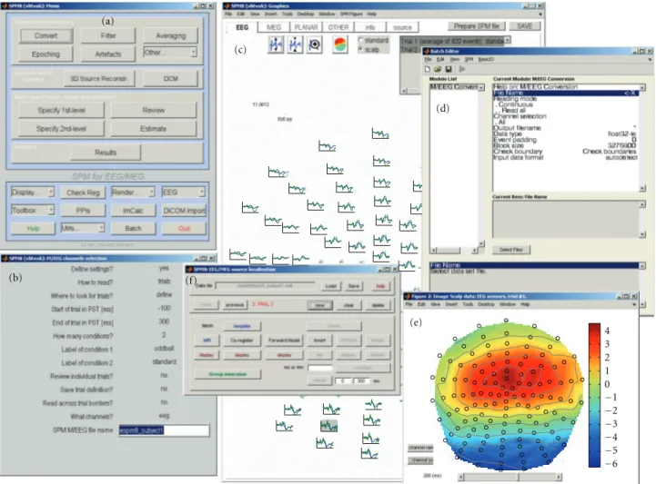
SPM for M/EEG can be invoked by typing spm eeg on the MATLAB command line and pressing Enter. After a brief initialization, the SPM GUI will appear. It consists
of three windows (see Figure 1). The menu window on
the top left (Figure 1(a)) contains buttons and other GUI
elements used to access different SPM functions. This
win-dow’s contents only change if the user switches modalities (fMRI/PET/MEEG). The interactive window (bottom left, Figure 1(b)) is used by SPM functions for creating dynamic GUI elements, when necessary (for instance, to present the user with a choice or ask for input). The graphics window on the right (Figure 1(c)) is where SPM presents intermediate and final results of its analyses. It is also used by the SPM M/EEG reviewing tool. Additional graphics windows are created when necessary.
There are three ways to access SPM M/EEG func-tionality. The first is to use the GUI. Since SPM8 is a GUI-based application, all the standard pre-processing and analysis procedures can be accessed this way with no need for programming. We recommend that beginners use the GUI first, because this will prompt SPM to ask for all relevant information needed to process the data. The second way is to use the matlabbatch tool (Figure 1(d)). Matlabbatch (http://sourceforge.net/projects/matlabbatch/) is a standalone batch system for MATLAB developed by Volkmar Glauche, based on the job manager, originally
4 3 2 1 0 −1 −2 −3 −4 −5 −6 (e) (b) (f)
Figure 1: SPM8 for M/EEG graphical user interface tools; see alsoFigure 11. (a) Menu window, (b) interactive window showing a series of inputs required for conversion of an EEG dataset, (c) graphics window with the SPM8 for M/EEG reviewing tool. Evoked responses recorded in a mismatch negativity experiment are displayed in a topographical plot, (d) MATLAB batch tool with the configuration interface for data conversion, (e) Scalp map of potential distribution for mismatch negativity data that was created from the reviewing tool, and (f) 3D source reconstruction interface.
developed for SPM5. Matlabbatch basically allows “program-ming without program“program-ming”. Processing pipelines can be built and configured using a specialized batch GUI and then applied to multiple datasets in noninteractive mode. The batch system is designed for repetitive analyses of data, once the user knows what should be done, and in which order. Matlabbatch can be accessed by pressing the “Batch” button in the SPM menu window. This will open the batch tool window. SPM functionality can be accessed via the “SPM” menu in this window. Finally, users familiar with MATLAB programming can call SPM functions directly from their scripts without using the GUI. We will refer to this way of using SPM as “scripting” as opposed to “batching”; that is, using the batch tool. The use of GUI, batching, and scripting are not always clearly separated, as for some functions the batch tool is the only available GUI. Also, batch pipelines can be created, modified, and run via scripts. In fact, creating a template batch and then invoking it from a script with specific inputs is the most convenient way to prescribe some of the more complicated analyses in SPM. Thus, SPM
scripts can combine the user’s own code with invoking SPM functions directly or via batch pipelines. The facilities used by SPM programmers to create dynamic GUIs and batch tools are also available to users for their own custom tools.
All the analysis procedures in SPM are optimized to reduce computation time: typically an analysis of a single dataset (e.g., source reconstruction or DCM) can be com-pleted in minutes (or in the worst case, tens of minutes) on a standard desktop computer. SPM does not require any special computer infrastructure or parallel computations, although one of our development directions is to introduce parallelization to finesse analysis of multiple subjects and fitting multiple alternative models to the data.
In what follows, we consider the three main domains in which SPM functionality is used. We start with analyses of M/EEG data in sensor space and then proceed to source space analyses in the subsequent sections. Typically, sensor-level analyses are used to identify peristimulus time or frequency windows, which are the focus of subsequent analyses in source space. These sensor space analyses use, effectively,
standard SPM procedures (topological inference) applied to a variety of electromagnetic data features that are organised into images.
3. Sensor-Level Analysis and
Topological Inference
EEG and MEG typically produce a time-varying modulation of signal amplitude or frequency-specific power in some peristimulus time period, at each electrode or sensor. Often, researchers are interested in whether condition-specific effects (observed at particular sensors and peristimulus times) are statistically significant. However, this inference must correct for the number of statistical tests performed. One way to do so is to control the family-wise error rate (FWER), the probability of making a false positive over the whole search space [24]. For independent observations, the FWER scales with the number of observations. A simple method for controlling FWER is the Bonferroni correction. However, this procedure is rarely adopted in neuroimaging because it assumes that neighbouring observations are independent. When there is a high degree of correlation among neighbouring samples (e.g., when data features are smooth), this correction is far too conservative.
Although the multiple comparisons problem has always existed for M/EEG analyses (due to the number of time bins in the peristimulus time window), the need for a correction method has become more acute with the advent of high-density EEG caps and MEG sensor arrays that increase the number of observations across the scalp. In many analyses, the multiple comparisons problem is circumvented by restricting the search space prior to inference, so that there is only one test per repeated measure. This is usually accomplished by averaging the data over prespecified sensors and time bins of interest. This produces one summary statistic per subject per condition. In many instances, this is a powerful and valid way to sidestep the multiple comparisons problem; however, it requires the space of interest to be specified a priori. A principled specification of this space could use orthogonal or independent data features. For example, if one were interested in the attentional modulation of the N170 (a typical event-related wave recorded 170 ms after face presentation), one could first define the electrodes and time bins that expressed an N170 (compared to baseline)
and then test for the effects of attention on their average.
Note that this approach assumes that condition-specific effects occur at the same sensors and time, and is only valid when selection is not biased [25]. In situations where the location of evoked or induced responses is not known a priori or cannot be localized independently, one can use topological inference to search over some space for significant responses; this is the approach implemented in SPM. It is based on the random field theory (RFT [4]). RFT provides a way
of adjusting the P-values that takes into account the fact
that neighbouring sensors are not independent, by virtue of continuity in the original data. Provided the data are smooth, the RFT adjustment is less severe (i.e., is more sensitive) than a Bonferroni correction for the number of sensors.
The theoretical basis of topological inference for M/EEG has been recently reviewed by Kilner and Friston [14]. Here, we rehearse some of the points from this review and provide more details about the SPM implementation of the method.
Statistical analyses of M/EEG data in SPM use the same mechanisms as all other data types (PET, fMRI, and structural MRI in VBM). This simply requires transforming data from SPM M/EEG format to image files (NIfTI
format,http://nifti.nimh.nih.gov/nifti-1/). Once the data are
in this image format, statistical analyses for M/EEG are procedurally identical to between-subject analyses of PET or VBM data (e.g., second level analyses in fMRI [26]). These analyses assume one summary statistic image per subject per condition (or level of an experimental factor). Here, a summary statistic image is just a technical term for the data feature summarising treatment effects that one wants to make an inference about. More formally, when this summary statistic is itself a maximum likelihood estimate based on within-subject data, the analysis is called a summary-statistic procedure for random effect models. In the present context, we will see that the summary statistic can comprise many different data features.
3.1. Creating Summary Statistics: Conversion to Images. This
function takes SPM M/EEG sensor data as input and gener-ates an image for each trial (for trials that were not rejected). This analysis can be applied to EEG and MEG (separately). In the case of MEG systems with planar gradiometers, images can be generated from root-mean-square values combining the two planar gradiometers at each location. In an averaged dataset, this will produce a single image per condition and enable statistical comparisons across subjects. In an epoched dataset, there will be an image per trial and multiple images per condition. It is, therefore, possible to perform within-subject statistical tests and then also take further summary statistic images (usually contrasts of parameter estimates from the within-subject models) from each subject to second level analyses between subjects.
3.1.1. Images over Time. Data in the time domain are
converted into an image by generating a scalp map for each time frame and stacking scalp maps over peristimulus
time (seeFigure 2). Scalp maps are generated using the 2D
sensor layout specified in the dataset (see Appendix B.3)
and linear interpolation between sensors. The user is asked to specify the output dimensions of the interpolated scalp map. Typically, we suggest 64 pixels in each spatial direction. There is also an option to either interpolate or remove bad channels from the images. Interpolation is the preferred option when there is a sufficient number of good channels around each bad channel. If bad channels are removed, there will be “holes” in the resulting images and these holes will be propagated throughout the statistical analysis. A directory is created with the same name as the input dataset. In this directory there will be a subdirectory for each trial type. These directories will contain 3D image files, where the
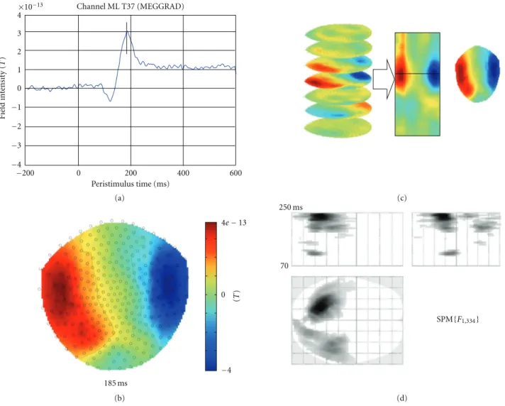
Peristimulus time (ms) −200 0 200 400 600 185 ms 250 ms 70 SPM{F1,334} 0 −4 (T ) 4e−13 (a) (b) (c) (d)
Figure 2: Construction of (space×space×time) summary statistic image and the ensuing SPM inference. The data are MEG responses to presentation of images of faces and scrambled faces. (a) Average ERF for a single subject recorded at a left temporal sensor in response to face presentation. The vertical line indicates the maximum positive value of this ERF. (b) Sensor-space map interpolated across all sensors at 185 ms after the stimulus, indicated by the line in (a). (c) Construction of a 3D (space×space×time) data volume from sensor-space maps, such as shown in (b). (d) Results of F test for difference between responses to faces and scrambled faces. Overall, single trials (168 for each condition) were converted to images as shown in (c). A two-samplet-test was performed and the results were assessed with an F-contrast to test for differences of either polarity. The results were thresholded at P =.05 with FWER correction based on random field theory. The red
arrow indicates the peak value of theF-statistic (at 245 ms).
averaged data (e.g., an event-related potential-ERP), a single image is placed in each directory. In the case of epoched data, there will be an image for each trial.
3.1.2. Averaging over Time. If the time window of interest is
known in advance (e.g., in the case of a well-characterized ERP or event-related field (ERF) peak) one can average over this time window to create a 2D image with just the spatial dimensions.
3.1.3. Time-Frequency Data. Although, in principle,
topo-logical inference can be done for any number of dimen-sions, the present implementation in SPM8 is limited to 3 dimensions or less. Thus, when time-frequency features are exported to summary statistic images, it is necessary to
reduce the data dimensionality from 4D (space×space ×
time ×frequency) to either a 3D image (space×space ×
time) or a 2D time-frequency image (time × frequency).
This is achieved by averaging either over channels (space
× space) or frequencies. Averaging over channels (or as a
common special case, selecting one channel) furnishes 2D time-frequency images (Figure 3).
When averaging over frequencies, one needs to specify the frequency range of interest. The power is then averaged over the specified frequency band to produce channel wave-forms. These waveforms are saved in a new time-domain M/EEG dataset. This dataset can be reviewed and further processed in the same way as ordinary time domain datasets (source reconstruction or DCM would not be appropriate because the data features are power or energy [21]). Once this
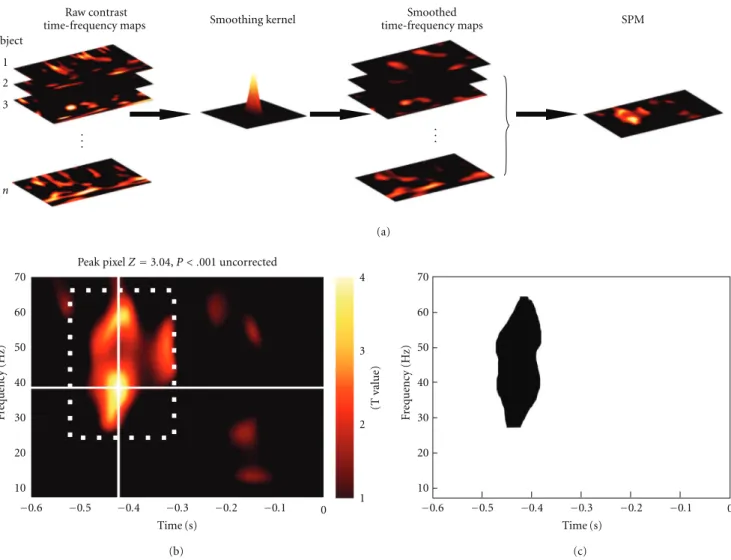
Subject 1 2 3 n Raw contrast
time-frequency maps Smoothing kernel
Smoothed time-frequency maps SPM . . . . . .
Peak pixelZ=3.04, P < .001 uncorrected
(T value) 1 2 3 4 −0.6 −0.5 −0.4 −0.3 −0.2 −0.1 0 Time (s) 10 20 30 40 50 60 70 10 20 30 40 50 60 70 −0.6 −0.5 −0.4 −0.3 −0.2 −0.1 0 Time (s) F requency (Hz) F requency (Hz) (a) (b) (c)
Figure 3: SPM analysis of time× frequency images. (a) Time-frequency images were calculated for each subject and smoothed by convolution with a Gaussian kernel. (b) At-statistic image was calculated from the smoothed time-frequency images and thresholded at
P < .01 (uncorrected). The location of the peak bin is shown. The white dotted box indicates our illustrative a priori window of interest. (c)
Statistical test restricted to the window of interest shown in (b) revealed a significant cluster (P =.005, cluster-level FWER correction). This
figure was adapted with permission from [15].
dataset is generated, it is automatically exported to images in the same way as data in the time domain (see above).
3.1.4. Smoothing. The images generated from M/EEG data
are generally smoothed prior to second level (i.e., group level) analysis by multidimensional convolution with a Gaus-sian kernel (standard image smoothing available in SPM). Smoothing is necessary to accommodate spatial/temporal variability over subjects and ensure the images conform to the assumptions of the topological inference approach. The dimensions of the smoothing kernel are specified in the units
of the original data: [mm×mm×ms] for space-time, [Hz
×ms] for time-frequency images. The guiding principle for
deciding how much to smooth is based on the matched filter theorem, which says that the smoothing kernel should match the scale of data features one expects. Therefore, the spatial extent of the smoothing kernel should be more or less similar to the extent of the dipolar patterns expected in the data
(probably of the order of a few cm). In practice, one can
try smoothing the images with different kernels, according
to the principle above; this is a form of scale space search or feature selection. Smoothing in time is not always necessary, as temporal filtering has the same effect. Once the images have been smoothed, one can proceed to the second level analysis.
Figure 2 is a schematic illustrating the construction of
(space × space × time) summary-statistic image and the
ensuing SPM testing for an effect of faces versus scrambled faces stimuli over subjects. This example highlights the role of topological inference (based on random field theory) to identify significant sensor-time regions that contain a
significant condition-specific response.Figure 3illustrates a
typical analysis in time × frequency space using a single
channel. These analyses can then be reported directly or used to finesse the subsequent characterisation of the appropriate peristimulus time window and frequency bands in source space.
mass univariate analysis in SPM, using appropriate summary statistic images over time and/or frequency.
In contrast to PET/fMRI image reconstruction, M/EEG source reconstruction is a nontrivial operation. Often com-pared to estimating a body shape from its shadow, inferring brain activity from scalp data is mathematically ill-posed and requires prior information such as anatomical, functional, or mathematical constraints to isolate a unique and highly probable solution [27]. Distributed linear models have been around for more than a decade now [28], and the recommended pipeline in SPM for an imaging solution is
very similar to common approaches in the field [29, 30].
However, at least three aspects are original and should be emphasized here.
(i) Based on an empirical Bayesian formalism, the inver-sion is meant to be generic, in the sense that it can incorporate and estimate the relevance of multiple constraints of a varied nature (i.e., it can reproduce a variety of standard constraints of the sort associated with minimum norm [29], LORETA [30], and other well-known solutions to the inverse problem). The
data-driven relevance of different constraints (priors)
is established through Bayesian model inversion, and
different sets of constraints can be evaluated using
Bayesian model comparison [16–18,31,32].
(ii) Subject-specific anatomy is incorporated in the gen-erative model of the data, in a fashion that eschews individual cortical surface extraction. The individ-ual cortical mesh is obtained automatically from a canonical mesh in MNI space, providing a simple and efficient way of reporting results in stereotactic coordinates [33].
(iii) SPM uses a Gaussian process model [34, 35] for
source reconstruction based on the sample channel×
channel covariance of the data over time. Crucially, this means it does not reconstruct one time bin at a time but uses the variance over time to furnish a full spatiotemporal inversion for each time series. This finesses any problems with specifying baselines, because only the variance (change from prestimulus baseline) contributes to the sample covariance and, therefore, the solution. In short, SPM reconstructs changes in source activity (not activity per se). This
(v) Summarizing the reconstructed response as an image.
Whereas the first three steps specify the forward or gen-erative model, the inverse reconstruction step is concerned with Bayesian inversion of that model and is the only step that requires the EEG/MEG data.
4.1. Getting Started. Everything described below is accessible
from the SPM user interface by pressing the “3D Source Reconstruction” button. A new window will appear with a GUI that guides the user through the necessary steps to obtain an imaging reconstruction of their data (see Figure 1(f)). At each step, the buttons not yet relevant for this step will be disabled. At the beginning, only two buttons are enabled: “Load”, which is used to load a preprocessed SPM M/EEG dataset and the “Group inversion” button that will be described below. One can load a dataset that is either epoched with single trials for different conditions, averaged with one ERP/ERF per condition, or grand averaged. An important precondition for loading a dataset is that it should contain sensors and fiducials (see “Section 4.3.”). This will be checked when loading a file and loading will fail if there is a problem. The user should make sure that for each modality in the dataset as indicated by channel types (either EEG or MEG), there is a sensor description. For instance, to load MEG data with some EEG channels that are not actually used for source reconstruction, the type of these channels should be changed to “LFP” (local field potential) or “Other” before trying to load the dataset. Unlike “Other” channels, “LFP” channels are filtered and are available for artefact detection. MEG data converted by SPM from their raw formats will usually contain valid sensor and fiducial descriptions. In the case of EEG, for some supported channel setups (such as extended 10–20 or Biosemi), SPM will provide default channel locations and fiducials that can be used for source reconstruction. Sensor and fiducial descriptions can be modified using the “Prepare” interface (seeAppendix B.3).
When a dataset is loaded, the user is asked to give a name to the reconstruction. In SPM, it is possible to perform multiple reconstructions of the same dataset with different parameters. The results of these reconstructions will be stored with the dataset after pressing the “Save” button. They can be loaded and reviewed using the “3D
Source Reconstruction” GUI and also with the SPM M/EEG reviewing tool. From the command line, one can access source reconstruction results via the D.inv field of the @meeg object. This field (if present) is a cell array of structures. Each cell contains the results of a different reconstruction. One can navigate among these cells in the GUI, using the buttons in the second row. One can also create, delete, and clear analysis cells. The label provided at the beginning will be attached to the cell for the user to identify it.
4.2. Source Space Modelling. After entering the label, the
“Template” and “MRI” buttons will be enabled. The “MRI” button creates individual head meshes describing the
bound-aries of different head compartments based on the subject’s
structural scan. SPM will ask for the subject’s structural image. It might take some time to prepare the model, as the image needs to be segmented as part of computing the nonlinear transformation from individual structural spaces to the template space [5]. The individual meshes are generated by applying the inverse of the spatial deformation field, which maps the individual structural image to the MNI template, to canonical meshes derived from this template
[33],Figure 4(b). This method is more robust than deriving
the meshes from the structural image directly and can work even when the quality of the individual structural images is low.
In the absence of an individual structural scan, com-bining the template head model with the individual head shape also results in a fairly precise head model. The “Template” button uses SPM’s template head model based on the MNI brain. The corresponding structural image can be found under canonical/single subj T1.nii in the SPM directory. When using the template, different things are done depending on whether the data are EEG or MEG. For EEG, the electrode positions will be transformed to match the template head. So even if the subject’s head is quite different from the template, one should be able to obtain reasonable results. For MEG, the template head will be transformed to match the fiducials and head shape that come with the MEG data. In this case, having a head shape measurement can be helpful in providing SPM with more data to scale the head correctly.
Irrespective of whether the “MRI” or “Template” button is used, the cortical mesh describing the locations of possible sources of the EEG and MEG signal is obtained from a template mesh (Figure 4(a)). In the case of EEG, the mesh is used as is, and in the case of MEG it is transformed with the head model. Three cortical mesh sizes are available: “coarse”, “normal”, and “fine” (5124, 8196, and 20484 vertices, resp.). We advise to work with the “normal” mesh. “Coarse” is useful for less powerful computers and “fine” will only work on 64-bit systems with enough main memory. The inner-skull, outer-inner-skull, and scalp canonical surfaces each comprise 2562 vertices, irrespective of the cortical mesh size.
For the purposes of forward computation, the orienta-tions of the sources are assumed to be normal to the cortical mesh. This might seem as a hard constraint at first glance, especially for the “Template” option, where the details of
the mesh do not match the individual cortical anatomy. However, in our experience, when a detailed enough mesh is used, the vertices in any local cortical patch vary sufficiently in their orientation to account for any activity that could come from the corresponding brain area; provided the mesh is sufficiently dense. All the (three) mesh resolutions offered
by SPM provide sufficient degrees of freedom in this context.
When comparing meshes with free and fixed orientation, Henson et al. [36] found the latter to be superior for SPM’s default source reconstruction method.
4.3. Data Coregistration. For SPM to provide a meaningful
interpretation of the results of source reconstruction, it should map the coordinate system in which sensor positions are originally represented to the coordinate system of a structural MRI (MNI coordinates).
There are two possible ways of coregistering M/EEG data to the structural MRI space.
(i) A landmark-based coregistration (using fiducials only). The rigid-body transformation matrices (rota-tion and transla(rota-tion) are computed such that they match each fiducial in the M/EEG space to the corresponding one in MRI space. The same transfor-mation is then applied to the sensor positions. (ii) Surface matching (between some head shape in
M/EEG space and some MRI-derived scalp tessella-tion).
For EEG, the sensor locations can be used instead of the head shape. For MEG, the head shape is first coregistered with MRI space; the inverse transformation is then applied to the head model and the mesh. Surface matching is performed using an iterative closest point algorithm (ICP). The ICP algorithm [37] is an iterative alignment algorithm that works in three phases.
(i) Establish correspondence between pairs of features in the two structures that are to be aligned, based on proximity.
(ii) Estimate the rigid transformation that best maps the first member of the pair onto the second.
(iii) Apply that transformation to all features in the first structure. These three steps are then reapplied until convergence. Although simple, the algorithm works quite effectively when given a good initial estimate. In practice, after pressing the “Coregister” button one needs to specify the points in the MRI that correspond to the M/EEG fiducials. If more than three fiducials are available (which may happen for EEG as, in principle, any electrode can be used as a fiducial), the user is asked at the first step to select the fiducials to use. It is possible to select more than three, but not less. Then for each M/EEG fiducial selected, the user is asked to specify the corresponding position in the MRI in one of three ways.
(i) “Select”—locations of some points such as the commonly used nasion and preauricular points and
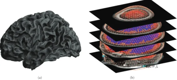
(a) (b)
Figure 4: Template meshes used for distributed source imaging. (a) “Normal” cortical template mesh (8196 vertices), left view. The triangular grid shows the representation of the cortical surface used by SPM. (b) All template meshes (cortex, inner skull, outer skull, and scalp) superimposed on the template MRI. Default fiducial locations associated with the template anatomy are displayed in light blue.
also CTF-recommended fiducials for MEG are hard-coded in SPM. If an M/EEG fiducial corresponds to one of these points, the user can select this option and then select the correct point from a list.
(ii) “Type”—here it is possible to enter the MNI
coordi-nates for the fiducial (1 ×3 vector). If the fiducial
is not in the SPM hard-coded list, it is advised to carefully find the correct point on either the template image or on the subject’s own image registered to the template. This can be done by opening the image using SPM’s image display functionality. One can then record the MNI coordinates and use them in subsequent coregistration, using the “type” option. (iii) “Click”—the user is presented with a structural
image and can click on the correct point. This option is good for “quick and dirty” coregistration or to try out different options.
After specifying the fiducials, the user is asked whether to use the head shape points if they are available. For EEG this is advised. For MEG, the head model is based on the subject’s MRI, and precise information about the fiducials is available (e.g., from a MRI with fiducials marked by vitamin E capsules); using the head shape might actually do more harm than good.
The results of the coregistration are presented in SPM’s
graphics window (seeFigure 5). It is important to examine
the results carefully before proceeding. The top panel shows the scalp, the inner skull, and the cortical mesh, with the sensors and the fiducials. For EEG one should make sure that the sensors are on the scalp surface. For MEG one should check that the head position, in relation to the sensors, makes sense and the head does not, for instance, protrude outside the sensor array. In the bottom panel, the sensor labels are shown in topographical array. One should check that the top labels correspond to anterior sensors, bottom to posterior, left to left, and right to right and also that the labels are where
expected topographically (e.g., that there is no shift when matching positions to channels).
4.4. Forward Computation. This refers to computing, for
each dipole on the cortical mesh, the effect it would have
on the sensors. The result is anN × M matrix where N is
the number of sensors andM is the number of mesh vertices
(chosen from several options at a previous step). This matrix can be quite large and is therefore stored in a separate MAT-file (whose name starts with “SPMgainmatrix”). This MAT-file is written to the same directory as the dataset. Each column in this matrix is a so-called “lead field”, corresponding to one mesh vertex. The lead fields are computed using the “forward” toolbox, which SPM shares with FieldTrip (see Oostenveld et al., this issue). This computation is based on Maxwell’s equations and makes assumptions about the physical properties of the head. There are different ways to specify these assumptions which are known as “forward models”.
The “forward” toolbox supports different forward
mod-els. After pressing the “Forward Model” button (which should be enabled after successful coregistration), the user has a choice of several head models, depending on the modality of the data. In SPM8, we recommend using a “single shell” model [38] for MEG and “EEG BEM” (Boundary Elements Model [39–43]) for EEG. One can also try other options and compare them using their model evidence ([36], see below). The first time the EEG BEM option is used with a new structural image (and also the first time the “Template” option is used) a lengthy computation will take place that prepares the BEM model based on the head meshes. The BEM will then be saved in a large MAT-file with ending “ EEG BEM.mat” in the same directory as the structural image (this is the “canonical” subdirectory of SPM for the template). When the head model is ready, it will be displayed in the graphics window, with the cortical mesh and
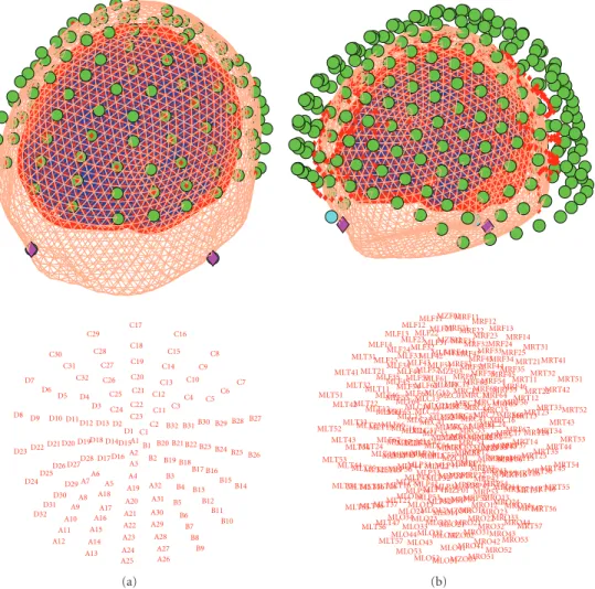
A1 A2 A3 A4 A5 A6 A7 A8 A9 A10 A11 A12 A13 A14 A15 A16 A17 A18 A19 A20 A21 A22 A23 A24 A25 A26 A27 A28 A29 A30 A31 A32 B1 B2 B3 B4 B5 B6 B7 B8 B9 B10 B11 B12 B13 B14 B15 B16 B17 B18 B19 B20 B21 B22 B23B24 B25 B26 B27 B28 B29 B30 B31 B32 C1C2 C3 C4 C5 C6 C7 C8 C9 C10 C11 C12 C13 C14 C15 C16 C17 C18 C19 C20 C21 C22 C23 C24 C25 C26 C27 C28 C29 C30 C31 C32 D1 D2 D3 D4 D5 D6 D7 D8 D9 D10 D11D12 D13 D14D15 D16 D17 D18 D19 D20 D21 D22 D23 D24D25 D26 D27D28 D29 D30 D31 D32 (a) MLC11 MLC12 MLC13 MLC14 MLC15 MLC16 MLC17 MLC21 MLC22 MLC23 MLC24 MLC25 MLC31 MLC32 MLC41 MLC42 MLC51 MLC52 MLC53 MLC54 MLC55 MLC61 MLC62 MLC63 MLF11 MLF12 MLF13 MLF14 MLF21 MLF22 MLF23 MLF24 MLF25 MLF31 MLF32 MLF33 MLF34 MLF35 MLF41 MLF42 MLF43 MLF44 MLF45 MLF46 MLF51 MLF52 MLF53 MLF54 MLF55 MLF56 MLF61 MLF62 MLF63 MLF64 MLF65 MLF66 MLF67 MLO11 MLO12 MLO13 MLO14 MLO21 MLO22 MLO23 MLO24 MLO31 MLO32 MLO33 MLO34 MLO41 MLO43 MLO44 MLO51 MLO52 MLO53 MLP11 MLP12 MLP21 MLP22 MLP23 MLP31 MLP32 MLP33 MLP34 MLP35 MLP41 MLP42 MLP43 MLP44 MLP45 MLP51 MLP52 MLP53 MLP54 MLP55 MLP56 MLP57 MLT11 MLT12 MLT13 MLT14 MLT15 MLT16 MLT21 MLT22 MLT23 MLT24 MLT25 MLT26 MLT27 MLT31 MLT32 MLT33 MLT34 MLT35 MLT36 MLT37 MLT41 MLT42 MLT43 MLT44 MLT45 MLT46 MLT47 MLT51 MLT52 MLT53 MLT54 MLT55 MLT56 MLT57 MRC11 MRC12MRC13 MRC14 MRC15 MRC16 MRC17 MRC21MRC22 MRC23 MRC24 MRC25 MRC31 MRC32 MRC41 MRC42 MRC51 MRC52 MRC53 MRC54 MRC55 MRC61 MRC62 MRC63 MRF11MRF12 MRF13 MRF14 MRF21MRF22 MRF23 MRF24 MRF25 MRF31MRF32 MRF33 MRF34 MRF35 MRF41MRF42 MRF43 MRF44 MRF45 MRF46 MRF51MRF52 MRF53 MRF54 MRF55 MRF56 MRF61 MRF62 MRF63 MRF64 MRF65 MRF66 MRF67 MRO11MRO12 MRO13 MRO14 MRO21MRO22 MRO23 MRO24 MRO31MRO32 MRO33 MRO34 MRO41MRO42 MRO43 MRO44 MRO51MRO52 MRO53 MRP11 MRP12 MRP21 MRP22 MRP23 MRP31 MRP32MRP33 MRP34 MRP35 MRP41MRP42 MRP43 MRP44 MRP45 MRP51MRP52MRP53 MRP54 MRP55 MRP56 MRP57 MRT11 MRT12 MRT13 MRT14 MRT15 MRT16 MRT21 MRT22 MRT23 MRT24 MRT25 MRT26 MRT27 MRT31 MRT32 MRT33 MRT34 MRT35 MRT36 MRT37 MRT41 MRT42 MRT43 MRT44 MRT45 MRT46 MRT47 MRT51 MRT52 MRT53 MRT54 MRT55 MRT56 MRT57 MZC01 MZC02 MZC03 MZC04 MZF01 MZF02 MZF03 MZO01 MZO02 MZO03 MZP01 (b)
Figure 5: Examples of coregistration display (appears after the co-registration step has been completed). Top row shows the 3D outcome of the co-registration, while the bottom row shows the sensor arrangement in 2D with corresponding labels. (a) EEG data (128 Biosemi system) from the multimodal face perception experiment available from the SPM website. EEG sensor locations have been adjusted to fit the scalp surface. (b) MEG data (275-channel CTF system) from the same experiment.
sensor locations, for verification (Figure 6). The actual lead field matrix is computed at the beginning of the next step and saved. This is a time-consuming step, particularly for high-resolution meshes. The lead field file will be used for all subsequent inversions, if the coregistration and the forward model are not changed.
4.5. Inverse Reconstruction. The inverse reconstruction is
invoked by pressing the “Invert” button. The first choice one gets is between “Imaging”, “VB-ECD”, and “DCM”. For reconstruction based on an empirical Bayesian approach (to localize evoked responses, evoked power, or induced power) one should press the “Imaging” button. The other options are explained in greater detail below. When there are several conditions (trial types) in the dataset, then the next choice is whether to invert all the conditions together or to choose a subset. If one is planning a statistical comparison between a set of conditions, one should invert all of them together. After selecting the conditions one gets a choice between “Standard” and “Custom” inversion. For “Standard”
inversion, SPM will start the computation with default settings. These correspond to the multiple sparse priors (MSP) algorithm [17], which is then applied to the whole time series.
To fine tune the parameters of the inversion, the “Cus-tom” option can be chosen. There will then be a possibility
to choose among several types of inversion, differing in
terms of their hyperpriors (priors on priors or constraints): IID—equivalent to classical minimum norm [29], COH— smoothness prior similar to methods such as LORETA [30], or multiple sparse priors (MSP) [17]. The latter gives the most plausible results and has been shown to have greater model evidence in relation to other priors [36].
One can then choose the time window that will be used for inversion. Based on our experience, we recommend the time window be limited to periods in which the activity of interest is expressed. The reason is that if irrelevant high-amplitude activity is included, source reconstruction will focus on reducing the error for reconstructing this activity and might suppress the responses of interest. There is also
(a) (b)
Figure 6: Examples of forward model display (appears after the forward modelling step has been completed). The figure includes the cortical mesh, the sensor locations and the other layers used to compute the lead-field matrix. (a) EEG data (128 Biosemi system) from the multimodal face perception experiment available from the SPM website. This figure shows the head model that was used to compute the BEM forward solution for these data. (b) MEG data (275-channel CTF system) from the same experiment. This figure shows the head model that was used to compute the realistic single shell solution for these data.
an option to apply a Hanning taper to the time series to down-weight possible baseline noise at the beginning and end of the trial. The next option is to prefilter the data. This is mainly for focusing on certain temporal scales during reconstruction (e.g., alpha band for ERPs or gamma for faster induced responses or sensory-evoked responses). The next option allows for extra source priors. This makes it possible to integrate prior knowledge from the literature or from fMRI/PET/DTI into the inversion [44]. Here, one can just provide a thresholded statistical image and SPM will generate the priors based on its suprathreshold clusters. Custom priors are not a “hard” way to restrict the solution. They will only be used when leading to a solution with higher model evidence. A “hard” restriction of the inverse solution is provided by the next option.
Here, one can restrict solutions to particular brain areas
by loading (or specifying) a MAT-file with a K × 3
matrix, containing MNI coordinates of the areas of interest. This option may seem strange initially; as it may seem to overly bias the source reconstruction. However, in the Bayesian inversion framework, it is possible to compare
different inversions of the same data using Bayesian model
comparison. By limiting the solutions to particular brain areas, one can greatly simplify the model, and if this simplification appropriately captures the sources generating the response, then the restricted model will have higher model evidence than the unrestricted one. If, however, the restricted sources cannot account for the data, the restriction will result in a worse model fit and the unrestricted model might be better (note that for model comparison to be valid, all settings that affect the data, like the time window and filtering, should be identical).
SPM8 imaging source reconstruction also supports mul-timodal datasets. These are datasets that have both EEG and MEG data from a simultaneous recording. Datasets from the
Elekta/Neuromag Vectorview MEG system, which has two kinds of MEG sensors, are also treated as multimodal. If the dataset is multimodal, a dialogue box will appear asking one to select the modalities for source reconstruction from a list. When selecting more than one modality, multimodal fusion will be performed. This option uses a heuristic to rescale the
data from different modalities so that they can be fused [45].
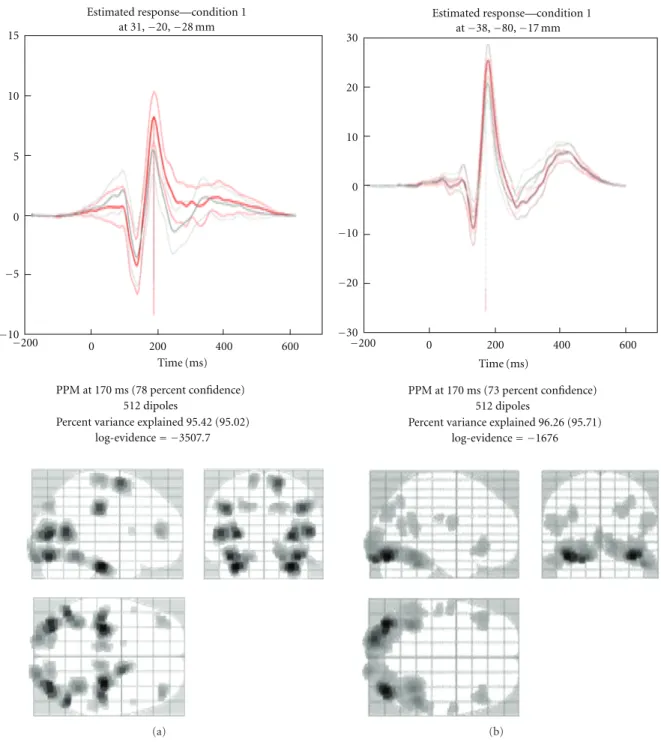
Once the inversion is complete, the time course of the source with maximal activity is presented in the top panel of
the graphics window (seeFigure 7). The bottom panel shows
the maximum intensity projection (MIP) at the time of the maximum activation. The log-evidence, which can be used for model comparison as explained above, is also shown. Note that not all of the output of the inversion is displayed. The full output consists of time courses for all the sources and conditions for the entire time window. It is possible to view more of these results using the controls in the bottom right corner of the 3D GUI. These allow one to focus on a particular time, brain area, and condition. One can also display a movie of the evolution of source activity.
4.6. Summarizing the Reconstructed Response as an Image.
SPM allows one to create summary statistic images in terms of contrasts (mixtures of parameter or activity estimates) over time and frequency. These are in the form of 3D NIfTI images, so that one can proceed to GLM-based statistical analysis in the usual way (at the between-subject level). This entails summarizing the trial- and subject-specific responses with a single 3D image in source space and involves specifying a time-frequency window for each contrast image. This is a flexible and generic way of specifying the data features one wants to make an inference about (e.g., gamma activity around 300 ms or average response between 80 and 120 ms). The contrast is specified by pressing the “Window”
15 10 5 0 −5 −10 −200 0 200 400 600 PPM at 170 ms (78 percent confidence) 512 dipoles
Percent variance explained 95.42 (95.02) log-evidence= −3507.7 Estimated response—condition 1 at 31,−20,−28 mm Time (ms) (a) −200 0 200 400 600 PPM at 170 ms (73 percent confidence) 512 dipoles
Percent variance explained 96.26 (95.71) log-evidence= −1676 −30 −20 −10 0 10 20 30 Time (ms)
Estimated response condition 1 at−38,−80,−17 mm
—
(b)
Figure 7: Display of the estimated distributed solution for evoked responses. The top panel shows the time course of the source having maximal activity while the bottom panel shows the maximum intensity projections (MIP) at the time of maximum activation. (a) EEG data from the multimodal face perception experiment available from the SPM website. (b) MEG data from the same experiment. Time course in red is for the face stimuli while the light grey is for scrambled faces. The lighter red and gray lines indicate 90% confidence intervals.
button. The user will then be asked about the time window of interest (in ms, peristimulus time). It is possible to specify one or more time segments (separated by a semicolon). To specify a single time point the same value can be repeated twice. The next prompt pertains to the frequency band. To average the source time course one can simply leave this at the default of zero. In this case, the window will be weighted by a Gaussian function. In the case of a single time point, this will be a Gaussian with 8 ms full
width half maximum (FWHM). If one specifies a particular frequency or a frequency band, then a series of Morlet wavelet projectors will be generated, summarizing the energy in the time window and frequency band of interest.
There is a difference between specifying a frequency band of interest as zero, as opposed to specifying a wide band that covers the whole frequency range of the data. In the former case, the time course of each dipole is averaged over time, weighted by a Gaussian. Therefore, if within the selected time
not be the same. The projectors specified (bottom panel of Figure 8) and the resulting MIP (top panel) will be displayed when the operation is completed. The “trials” option makes it possible to export an image per trial, which is useful for performing parametric within-subject analyses (e.g., looking for the correlates of reaction times).
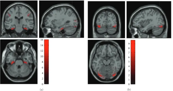
The values of the exported images are normalized to reduce between-subject variance. Therefore, for best results one should export images for all the time windows and con-ditions that will be included in the same statistical analysis together. Note that the images exported from the source reconstruction are a little peculiar because of smoothing from a 2D cortical sheet into 3D volume (Figure 9). SPM’s statistical machinery has been optimized to deal with these peculiarities and ensure sensible results.
In what follows, we consider some auxiliary functions associated with source reconstruction.
4.6.1. Rendering Interface. By pressing the “Render” button
one can open a new GUI window, which displays a rendering of the inversion results on the brain surface. One can rotate
the brain, focus on different time points, run a movie, and
compare the predicted and observed scalp topographies and time series. A useful option is the “virtual electrode”, which allows one to extract the time course from any point on the mesh and form the MIP at the time of maximum activation at this point. An additional tool for reviewing the results is available in the SPM M/EEG reviewing tool.
4.6.2. Group Inversion. A problem encountered with MSP
inversion is that it sometimes produces solutions that are so focal in each subject that the spatial overlap between the activated areas across subjects is not sufficient to yield a significant result at the between-subject level. This could be finessed by smoothing, but smoothing compromises the spatial resolution and thus subverts the main advantage of using an inversion method that can produce focal solutions. The more principled solution is to tell the model that the same distributed brain system has been engaged in all subjects or sessions (by design). This is simple to do using a hierarchical extension of the MSP method [46] that effectively ensures the activated sources are the same in all subjects (only the time course of activation is allowed to vary over subjects). We showed that this modification makes
this is straightforward because the linear mappings from each subject’s sensors to a canonical set of cortical sources imply there is a unique linear mapping from one subject’s montage to another; in other words, we can compute what we would have seen if one subject had been studied with the montage of another subject. However, in practice, the requisite realignment is a little more difficult because the “average” montage must converse information from all subjects. Imagine that two subjects have been studied with a single electrode and that the lead fields of these two electrodes are orthogonal. This means that realigning the sensor from one subject with the other would lose all the information from the subject being realigned. What we seek is an average sensor that captures the signals from both subjects in a balanced way. This can be achieved by iteratively solving a set of linear equations under the constraint that the mutual information between the average (realigned) sensor data and each subject’s data is maximized. SPM8 uses a recursive (generalised) least squares scheme to do this.
Group inversion can be started by pressing the “Group inversion” button right after opening the 3D source recon-struction GUI. The user is asked to specify a list of M/EEG datasets to invert together. Then one is asked to coregister each of the files and specify all the inversion parameters in advance. It is also possible to specify contrasts in advance. Then the inversion will proceed by computing the inverse solution for all the files and will write out the output images. The results for each subject are saved in the header of the corresponding input file. It is possible to load this file into the 3D GUI, after inversion, and explore the results as described above.
4.6.3. Batching Source Reconstruction. One can also run
imaging source reconstructions using the matlabbatch tool. It can be accessed by pressing the “Batch” button in the main SPM window and then going to “M/EEG source reconstruction” under “SPM” and “M/EEG”. There are three separate tools here for building head models, computing the inverse solution and creating contrast images. This makes it possible to generate images for several different contrasts from the same inversion. All the three tools support multiple datasets as inputs. Group inversion is used automatically for multiple datasets.
Condition 1 energy (evoked) 256 voxels −0.5 −0.4 −0.3 −0.2 −0.1 0 0.1 0.2 0.3 0.4 C o nt rast PST (ms) −200 0 200 400 600 (a) Condition 1 energy (evoked) 256 voxels −0.5 −0.4 −0.3 −0.2 −0.1 0 0.1 0.2 0.3 0.4 C o nt rast PST (ms) −200 0 200 400 600 (b)
Figure 8: Display of the estimated distributed solution for evoked power in a specific frequency band. The same can be obtained for induced power and for each trial. The top panel shows the maximum intensity projections (MIP) while the bottom panel shows the applied time-frequency contrast. (a) EEG data from the multimodal face perception experiment available from the SPM website. (b) MEG data from the same experiment. Evoked power was computed between 150 and 200 ms, for frequencies between 1 and 20 Hz.
This completes our review of distributed source recon-struction. Before turning to the final section, we consider briefly the alternative sort of source space model, which is much simpler but, unlike the cortical mesh described in this section, leads to a nonlinear forward model parametrisation.
5. Localization of Equivalent Current Dipoles
This section describes source reconstruction based on Variational bayesian equivalent current dipoles (VB-ECDs) [19]. 3D imaging (or distributed) reconstruction methods
consider all possible source locations simultaneously, allow-ing for large and distributed clusters of activity. This is to be contrasted with “equivalent current dipole” (ECD) approaches, which rely on two hypotheses.
(i) Only a few (say less than ∼5) sources are active
simultaneously, and that (ii) those sources are focal.
This leads to the ECD forward model, where the observed scalp potential is explained by a handful of discrete current sources; that is, dipoles, located inside the brain volume.
0 2 4 6 8 (a) 5 4 3 2 1 0 (b)
Figure 9: Axial, sagittal, and coronal views of the contrast image shown inFigure 8, projected into MNI voxel space and superimposed on the template structural MRI image. (a) EEG data from the multimodal face perception experiment available from the SPM website. (b) MEG data from the same experiment. The intensity was normalised to the mean over voxels to reduce intersubject variance.
In contrast to imaging reconstruction, the number of ECDs considered in the model, that is, the number of active loca-tions, has to be defined a priori. This is a crucial step, as the number of sources considered defines the ECD model. This choice should be based on empirical knowledge about the brain activity observed or any other source of information (e.g., by looking at the scalp potential distribution). Note that the number of ECDs can be optimised post hoc using model comparison (see below). In general, each dipole is described by six parameters: three for its location, two for its orientation, and one for its amplitude. To keep the inverse problem overdetermined, the number of ECDs therefore must not exceed the number of channels divided by 6, and preferably should be well below this threshold. Once the number of ECDs is fixed, a nonlinear Variational Bayesian scheme is used to optimise the dipole parameters (six times the number of dipoles) given the observed potentials.
Classical ECD approaches use a simple best fitting optimisation using “least square error” criteria. This leads to relatively simple algorithms but presents a few drawbacks.
(i) Constraints on the dipoles are difficult to include in the framework.
(ii) Noise cannot be properly taken into account, as its variance should be estimated alongside the dipole parameters.
(iii) It is difficult to define confidence intervals on the estimated parameters, which could lead to overcon-fidence in the results.
(iv) Models with different numbers of ECDs cannot
be compared, except through their goodness-of-fit,
which can be misleading. As adding dipoles to a model will necessarily improve the overall goodness of fit, one could erroneously be tempted to use as many ECDs as possible and to perfectly fit the observed signal.
However, using Bayesian techniques, it is possible to cir-cumvent all of the above limitations of classical approaches. Briefly, a probabilistic generative model is built, providing a likelihood model for the data. This assumes an independent and identically distributed normal distribution for the errors, but other distributions could be specified. The model is completed by priors on the various parameters, leading to a Bayesian forward model, which allows the inclusion of user-specified prior constraints.
An iterative Variational Bayesian scheme is then employed to estimate the posterior distribution of the parameters (in fact the same scheme used for distributed solutions). The confidence interval on the estimated param-eters is therefore directly available through the posterior variance of the parameters. Crucially, in a Bayesian context, different models can be compared using their evidence. This model comparison is superior to classical goodness-of-fit measures, because it takes into account the complexity of the models (e.g., the number of dipoles) and, implicitly, uncertainty about the model parameters. VB-ECD can therefore provide an objective and accurate answer to the question: would this dataset be better modelled by two or three ECDs? We now describe the procedure for using the VB-ECD approach in SPM8.
The engine calculating the projection (lead field) of the dipolar sources to the scalp electrodes comes from FieldTrip
and is the same for the 3D imaging or DCM. The head model should thus be prepared the same way, as described in the previous section. For the same data set, differences between the VB-ECD and imaging reconstructions are, therefore, only due to the reconstruction chosen.
5.1. VB-ECD Reconstruction. After loading and preparing
the head model, one should select the VB-ECD option after pressing the “Invert” button in the “3D source reconstruc-tion” window. The user is then invited to fill in information about the ECD model and click on buttons in the following order.
(i) Indicate the time bin or window for the reconstruc-tion. Note that the data will be averaged over the selected time window. VB-ECD will thus always be calculated for a single scalp topography.
(ii) Enter the trial type(s) to be reconstructed. Each trial type will be reconstructed separately.
(iii) Add a single (i.e., individual) dipole or a pair of symmetric dipoles to the model.
(iv) Select “Informative” or “Noninformative” location priors. “Non-informative” invokes flat priors over the brain volume. With “Informative”, one can enter the a priori location of the source (for a symmetric pair of dipoles, only one set of dipole coordinates is required).
(v) At this point, it is possible to go back and add more dipole(s) to the model, or stop adding dipoles. (vi) Specify the number of iterations. These are
repeti-tions of the fitting procedure with different initial
conditions. Since there are multiple local maxima in the objective function, multiple iterations are necessary to ensure good results, especially when non-informative location priors are chosen.
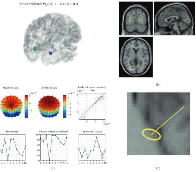
The routine then proceeds with the VB optimization scheme to estimate the model parameters. There is a graphical display of intermediate results. When the best solution is selected, the model evidence will be shown at the
top of the SPM graphics window (see Figure 10(a)). This
can be used to compare solutions with different priors or number of ECDs. Results of the inversion are saved to the data structure and displayed in the graphics window.
5.1.1. Result Display. The VB-ECD results can be displayed
again by pressing the “dip” button, located under the “Invert” button that will be enabled after computing VB-ECD solution. In the upper part, the three main figures display orthogonal views of the brain with the dipole
location and orientation superimposed (see Figure 10(b)).
The location confidence interval is reported by the dotted ellipse around the dipole location (Figure 10(c)). The lower left table displays the current dipole location, orientation (Cartesian or polar coordinates), and amplitude in various formats. The lower right table allows for the selection of trial types and dipoles. Display of multiple trial types and
multiple dipoles is also possible. The display will centre itself on the average location of the dipoles.
This completes our discussion of source reconstruc-tion. The previous sections introduced distributed and ECD solutions based on forward models mapping from sources to sensors. These models are not constrained to produce physiologically plausible neuronal activity estimates
and ignore the neuronal coupling among different dipolar
sources in generating observed sensor signals. In the final section, we turn to dynamic causal modelling (DCM),
which effectively puts a neuronal model underneath the
electromagnetic forward models considered above. Usually, source reconstruction (imaging or ECD) is used to answer questions about the functional anatomy of evoked or induced responses, in terms of where sources have been engaged. This information is generally used to specify the location priors of sources in DCM.
6. Dynamic Causal Modelling for M/EEG
Dynamic causal modelling (DCM) is based on an idea initially developed for fMRI data [8]. Briefly, measured data are explained by a network model consisting of a few sources, which are dynamically coupled (cf. spatiotemporal dipole
modelling introduced by Scherg and colleagues [47, 48]).
This network model is inverted using the same Variational Bayesian scheme used for source reconstruction. Model inversion furnishes the model evidence (used to search model spaces or hypotheses) and the posterior density on model parameters (used to make inferences about connec-tions between sources or their condition-specific modula-tion), under the model selected. David et al. [20] extended the DCM idea to modelling ERPs. At its heart DCM for ERP (DCM-ERP) is a source reconstruction technique, and for the spatial domain we use exactly the same forward model as the approaches in previous sections. However, what makes DCM unique is that it combines the spatial forward model with a neurobiologically informed temporal forward model, describing the connectivity among sources. This crucial ingredient not only makes the source reconstruction more robust, by implicitly constraining the spatial parameters, but also allows inference about connectivity architectures.
For M/EEG data, DCM can be a powerful technique for inferring (neuronal) parameters not observable with M/EEG directly. Specifically, one is not limited to ques-tions about source strength, as estimated using a source reconstruction approach, but can test hypotheses about connections between sources in a network. As M/EEG data are highly resolved in time, as compared to fMRI, precise inferences about neurobiologically meaningful parameters (e.g., synaptic time constants) are possible. These relate more directly to the causes of the underlying neuronal dynamics. In the recent years, several variants of DCM for M/EEG have been developed. DCM for steady state responses
(DCM-SSR) [22, 49, 50] uses the same neural models as
DCM-ERP to generate predictions for power spectra and cross-spectra measured under steady state assumptions. There are also (phenomenological) DCMs that model specific data features, without an explicit neural model. DCM for
×10−6 ×10⁻⁶ 5 0 −5 ×10−6 ×10−6 5 5 0 0 −5 −5 2 0 −2 −4 −6 −8
Free energy Percent variance explained Dipole amp (nAm) Measured data Predicted data
1 2 3 4 5 6 7 8 9 10 01 2 3 4 5 6 7 8 9 10 1 2 3 4 5 6 7 8 9 10 20 40 60 80 100 (a) (b) (c)
Predicted versus measured data
Figure 10: VB-ECD solution illustrated here on EEG data from the multimodal face perception experiment available from the SPM website. A symmetric dipole pair was fitted to the topography of the difference between faces and scrambled faces averaged between 170 and 180 ms. (a) The upper part shows the dipole location through the transparent cortical mesh; the middle part shows the correspondence between observed and predicted scalp data in two ways (topographies and dot plot); the bottom part shows the free energy, the explained variance, and the estimated dipole amplitude (from left to right) obtained from each of the ten repetitions of the procedure with different initial locations. Results correspond to the one with highest free energy (red point). (b) Orthogonal views of the brain with dipole locations obtained from the solution with highest free energy. (c) Enlarged fragment of the axial image shown by white square in (b). The ellipse shows the 95% confidence volume for dipole location.
induced responses (DCM-IR) [21] models event-related power dynamics (time-frequency features). DCM for phase coupling (DCM-PHA) [23] models event-related changes in phase relations between brain sources: DCM-PHA can be applied to one frequency band at a time. Presently, all M/EEG DCMs share the same interface, as many of the variables that need to be specified are the same for all four approaches. Therefore, we will focus on DCM for evoked responses and then point out where the differences to the other DCMs lie.
In this section, we only provide a procedural guide for the practical use of DCM for M/EEG. For the scientific background, the algorithms used or how one would typically use DCM in applications, we recommend the following. A general overview of M/EEG DCMs can be found in [51].
The two key technical contributions for DCM-ERP can be
found in [20, 52]. Tests of interesting hypotheses about
neuronal dynamics are described in [53,54]. Other examples
of applications demonstrating the kind of hypotheses testable
with DCM can be found in [55,56]. Another good source
of background information is the recent SPM book [57] where parts 6 and 7 cover not only DCM for M/EEG but contextualise DCM with related research from our group.
DCM-IR is covered in [21,58], DCM-SSR in [22,49,50],
and DCM-PHA in [23].
6.1. Overview. The goal of DCM is to explain measured
data (such as evoked responses) as the output of an inter-acting network consisting of several areas, some of which