Elastic behavior of bolted connection between cylindrical steel
structure and concrete foundation
Hoang Van-Long, Jaspart Jean-Pierre, Demonceau Jean-François ArGEnCo Department, University of Liège, Belgium
Corresponding author:
Hoang Van Long
Chemin des Chevreuils, 1 B52/3, 4000 Liège, Belgium Phone: +3243669614
E-mail: s.hoangvanlong@ulg.ac.be
Key words: cylindrical structures; column base; bolted connections; elastic behaviour; component method
Highlights
Bolted cylindrical steel structures – concrete foundation connection is investigated
An analytical model to obtain the elastic response of the connection is proposed The effect of the bolt preloading is taken into account
The long time and volume behaviours of concrete is considered The calculation procedure is given with illustrative examples
Abstract: the paper deals with bolted connection between cylindrical steel structures and concrete foundations. In the considered connection, the circular steel structure of
large diameter is welded to a base plate, and then anchor bolts are used to connect the
base plate to the concrete foundation. Repartition plates are also placed to ensure an
appropriate distribution of the stresses from the steel parts into the concrete. The
studied configuration is often met in industrial chimneys, wind towers, cranes, etc. To
but no appropriate and efficient tools for the characterisation of its elastic behaviour
are available in the codes and literatures.
In the present paper, a complete analytical procedure is proposed to predict the elastic
responses of the connection from their geometrical and material characteristics.
Several effects are taken into account in the model, such as the effect of the bolt
preloading, the long term effects in the concrete and 3D behaviour of the concrete
foundation. The analytical results are validated through comparisons with numerical
results. Numerical examples are also given to illustrate the proposed calculation
procedure.
Notations
Materials
Es and s are the Young modulus and Poisson ratio of the steel plates respectively
Eb is the Young modulus of bolt material
Ec and c are the Young modulus and Poisson ratio of the concrete respectively (t) is the creep coefficient of the concrete at time t
shrinkage is the deformation due to the shrinkage of the concrete at time t
Geometrical parameters
a1 is the distance from the base plate edge to the repartition plate edge (the wall side)
a2 is the distance from the base plate edge to the repartition plate edge (the free side)
b is the width of the sub-part (equals to the base/repartition plate width) beff is the effective width of the base plate
d is the nominal diameter of the bolt dw is the diameter of the washer
e01 is the distance from the bolt centre to the prying force position (with preload effect)
e02 is the distance from the bolt centre to the prying force position (without preload
effect)
e1 is the distance from the centre of the tube wall to the bolt centre
e2 is the distance from the bolt centre to the free edge of the base plate
ex is the distance from the centre of the tube wall to the base plate edge
Hc is the height of the concrete part between two repartition plates
lb is the grip length of the bolt
rw is the radius of the tube wall (structure body)
rb is the radius of the bolt pitch
tb is the thickness of the base plate
tp is the thickness of the repartition plate
tw is the thickness of the tube wall
w is the width of the repartition plate
wr is the width of the rigid part of the repartition plate
Forces
B0 is the initial preload in the bolt
B1 is the force in the bolt from which the preload effect is absence
Ft and Fc are respectively the tension and compression forces applied to the sub-part
F1 is the tension force from which the preload effect is absence
M is the bending moment applied to the whole connection Mb is the bending moment in the bolt shank (at the bolt head)
Mw is the bending moment in the tube wall (at the section attached to the base plate)
N is the axial force applying to the whole connection Rigidities
EsI is the bending rigidity of the base plate (equivalent beam)
GsA is the shear rigidity of the base plate (equivalent beam)
k,b is the rigidity of the bolt in tension
k,b is the rigidity of the bolt in bending
k, c is the rigidity of the concrete under compression
k, c is the rigidity of the concrete under bending
kw is the flexural rigidity of the tube wall
Kt1 is the rigidity of the sub-part in tension with the preload effect
Kt2 is the rigidity of the sub-part in tension without the preload effect
Kc is the rigidity of the sub-part in compression
1. Introduction
Normally, cylindrical steel structures with large diameters, such as industrial
chimneys, wind towers, cranes, etc., are connected to a concrete foundation by a bolted
joint (Fig.1). For this type of connection, the body of the structure is welded to a base
plate, and then the anchor bolts are used to connect the base plate to the foundation.
Repartition plates are also placed to ensure an appropriate distribution of stresses from
the steel parts into the concrete foundation.
Globally, this type of structure works as a cantilever beam; therefore, the
behaviour of the structure. Moreover, experience shows that the base connection of the
structure is the zone where premature failures often occur, mainly due to fatigue in the
bolts. So the design and execution of the structure-foundation connection require an
important vigilance.
Since the diameter of the assembly is very large (about 2 m to 6 m), and the bending
effect is predominant in the structure body, the use of a plastic model would result in
important ductility requirements that most configurations could not meet in the
practice. Therefore, an elastic approach appears to be the most relevant one. In
addition, an elastic model can provide useful information, as the connection rigidity,
the evolution of the stress in the elements. These information allow to assess the
fatigue strength or calculate static/dynamic responses of the structure in the design
process.
Concerning the design codes, the following remarks can be drawn: EN-1993-1-8
(design of joints) [8] provides rules for calculating column bases, especially for
columns in buildings with I / H sections. So, improvements of these rules is required in
order to cover the joint configuration investigated here. EN-1993-1-9 dedicated to
fatigue design [9] provides us details to estimate the fatigue resistance of elements of
steel structures. The bolt is classified as a nominal detail for which the effects of
bending and prying must be considered. However, the determination of the stress in
the bolt taking into account these effects in the elastic range is questionable in many
cases. Other codes may be considered, such as CEN/TS1992-4-1 (Design of
or EN1993-4-1 (Design of Silos) [12] but they do not specifically address the design of
connections between cylindrical structures and concrete foundations.
Looking in literature, several researches regarding the behaviour of column bases [e.g.
13, 14, 16, 17, 19, 20, 21, among others] have been carried out in the past 20 years.
Most of them investigate the possibility to extend the component method (initially
developed for beam-to-column) to column bases of buildings with columns with I, H
or hollow sections. The application of these results on the analysis of cylindrical
structures, especially in the elastic range, require more developments. In particular, the
presence of bolt preloading is not addressed in the existing tools, due to a lack of
knowledge in terms of loss of preload in the anchor bolt.
Due to the above mentioned reasons, engineers encounter difficulties when designing
the considered type of assembly and sophisticated numerical model through finite
element methods is often used, even it is known to be expensive and time consuming.
In the present paper, a complete analytical procedure is proposed to predict the elastic
responses of the connection from their geometrical and material characteristics. Several
effects are taken into account in the model, such as the effect of the bolt preloading, the
long term effects in the concrete and 3D behaviour of the concrete foundation. The
analytical results are validated through comparisons to numerical results. Numerical
examples are also given to illustrate the proposed calculation procedure.
2. Behaviour of a sub-part of the connection
As the considered connection is axis-symmetric (both geometry and material), the
studies may be carried out on a sub-part, as described in Fig.2; this is a 1/n part with n,
this means that the shape of the plates is quite complex. However, for sake of
simplicity, a rectangular form is adopted for the conducted investigations. As the
diameter of the connection and the number of bolts are normally significant, the above
assumption leads to negligible uncertainties. The width, b, of the sub-part may be
estimated as the arc length at the level of the bolts (place on a circle with a radius rb –
see Fig.2 ), meaning that b may be calculated by Eq.(1).
2 rb b
n
(1)
When the whole structure is subjected to external loads (i.e. horizontal and vertical
loads), the tension/compression forces are transferred to the sub-part through the
structure wall. Accordingly, based on the component method concept, the following
components should be considered to obtain the behaviour of the sub-part:
Structure wall in traction/compression and bending Base plate in flexion and shear
Bolt in tension and bending Repartition plate in bending Concrete in compression
The mentioned components will be characterized in Section 2.1. The procedure to
obtain the global behaviour of the sub-part will be presented in Section 2.2. Then, the
asseembly procedure of the sub-part to obtain the whole joint behaviour will be dealt
with in Section 3. The calculation procedure will be summarized in Section 4. Section
5 aims at validating the proposed method and at illustrating the calculation procedure.
2.1. Behaviour of individual components
2.1.1. Structure wall component
The structure wall plays two roles (Fig.3): (1) transfer the tension/compression
force from the structure body to the base plate; and (2) restrain the rotation of the
base plate. Within the proposed model, the second role is considered by simulating
the restraining effect through an elastic rotational spring with an appropriate
rigidity kw. To determine kw, the structure body is modelled by a cylindrical shell
with an infinitive length; the centripetal displacement at the end of the cylindrical
shell is blocked by the base place. kw is defined as the ratio between the applied
moment and the rotation at the end of the shell wall. Through classical mechanical
approaches, it is easy to deduce the following equation for kw (details of the
intermediate quantities may be found in [18]):
2
wk
Db
(2) with
3 2 12 1 s w s E t D v , the bending rigidity of the shell and 4 2 4 s w w E t r D where Es and s
are respectively the Young modulus and the Poisson coefficient of the steel tube, rw
and tw are the radius and the thickness of the steel tube and b is the width of the
sub-part.
2.1.2. Base plate component
The behaviour of the base plate is similar to the flange of a standard T-stub as
defined in the component method [8]. Therefore, the base plate may be modelled
by an equivalent beam with a section width equals to 0.85b (Fig.4), as
0.85
eff
b b (3)
2.1.3. Anchor bolt component
In the present work, the two following specificities are recommended for the anchor
bolts:
(1) In many cases, a nut is placed under the repartition plate to facilitate the
build-up procedure; however, with the presence of this nut, most of the bolt length is
not preloaded (Fig.5), meaning that the fatigue resistance is considerably
reduced (the fatigue often occurs just under the mentioned nut). So, it is
recommended here to place no nut under the repartition plate.
(2) A direct contact between the bolt and the concrete results in a concentration of
stresses in the bolt shank (Fig.6), reducing also the fatigue resistance of the
bolts. So, it is recommended here to avoid such contact by placing, for instance,
plastic tubes around the bolts shank before the concrete casting procedure may
be used.
Considering the two above mentioned specificities, the bolt may be modelled as a
clamped-pinned bar, as seen in Fig.7. The length (lb) of the bar is considered as
equal to the distance between the lower face of the lower reparation plate and the
upper face of the base plate (Fig.7); this corresponds to the grip length of the bolt.
By using this model, the rigidities in tension and flexion of the bolt can be
formulated. As the tension force in the bolt is important, it is recommended to take
into account the effect of the tension force on the rigidity in flexion by using the
stability functions. Accordingly, the rigidity in tension rigidity (k,b) and the
, b b b b E A k l (4) , b b b b E I k S l (5)
In Eqs.(4) and (5), Eb is the Young modulus of the bolt material; lb is the bolt
length (Fig.7); Ab and Ib are the area and the second moment of the cross-section of
the bolt respectively(of the threated or non-threated portion according to the bolt
configuration). S is the stability function that can be found in many references (e.g
[2]):
2 cosh sinh 2 2 cosh sinh b b b b b b b kl kl kl kl S kl kl kl (6)with k B E I/ b b where B is the force in the bolt, and EbIb is the flexion modulus of
the bolt. In fact, B varies according to time (due to loss of preloading and due to
external load); for the sake of simplification, the initial value B0 may be adopted, B0
being equal to the initial preloading subtracting the loss associated to the creep and
shrinkage of the concrete. The details on the loss part will be dealt with in Section
2.1.6. For practical purpose, some concrete values of the stability function are given
in Table 1.
2.1.4. Repartition plate component
In the calculation of the column bases, the flexible plate in contact with the
concrete is normally replaced by a rigid plate. In this work, a model based on the
equivalent rigid plate proposed in [16] is applied, in which equivalence condition
on the displacement between the flexible and rigid plates (Fig.8) is adopted, and the
3 0, 66 s p c E c t E (7)
In Eq.(7), Es and Ec are the Young modulus of the repartition plate and of the
concrete respectively; tp is the thickness of the repartition plate. In the case where
Es=210000 N/mm2 and Ec=300000 N/mm2 , one has c 1.25tp.
With the present case, two situations can be identified, depending on the
considered contact zone between the base plate and the repartition plate:
(1) A punctual contact for which the contact zone is simplified as a line (Figs.
9a and 9b); this situation is met in the case of a free contact between the plate and
the repartition plate.
(2) A contact zone spreading on a certain area (Figs. 9c and 9d) in situation
where the contact between the two plates is imposed by the bolt. The nut (or bolt
head) is considered as rigid and a 45 degree diffusion is assumed in the base plates.
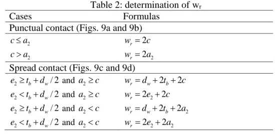
From the above assumptions and the actual geometries of the plates, the dimension
of the rigid part of the repartition plate can be obtained (Table 2).
2.1.5. Concrete block component
In EN-1993, part 1.8 [8], the rigidity of the concrete block is given by:
_ _ , 1.275 c eff EN eff EN c EN E b l k
with Ec, the concrete Young modulus; beff_EN and leff_EN, respectively the width and
the length of the effective part of the repartition plate (or base plate if a repartition
The following assumption have been used in EN-1993, part 1.8 [8] to deduct the
above expression for the rigidity of the concrete:
A coefficient of 1.5 is used to reduce the rigidity in order to consider the poor quality of the concrete surface in contact with the plate.
The concrete block is considered as a half elastic space, a coefficient with a fixed value of 0.85 is used to take into account the dimensions (beff_EN and
leff_EN) of the effective plate (rigid plate). This means that the different
dimensions of the plate are disregarded.
For the present case, it is proposed that:
The quality of the concrete at the surface between the concrete and the repartition plate is supposed to be “perfect”, meaning the reduction on the
rigidity is not required (i.e. the reduction coefficient equals to 1.0). This
assumption is based on the fact that the repartition plate is directly embedded in
the concrete; this plate is placed before the concrete casting.
The volume effect should be considered for each case, depending on the dimensions of the rigid plate and the concrete block. This consideration is
performed as explained here after.
As a sub-part is extracted from the whole connection (Fig.2), the lateral
deformation of the sub-part is locked; a plane deformation behavior may be
adopted, meaning that the 3D problem becomes a 2D problem. Moreover, it is
plate is considered (Hc in Fig.10). The actual width (Lc) of the concrete, symmetric
with respect to the rigid plate (Fig.10), is taken into account in the model.
The rigidity of the concrete block may be obtained through the expression (8):
, c c E k b (8)
with Ec, the concrete Young modulus; b, the width of the sub-part (Eq.(1)); , a
coefficient taking into account of the volume effect, depending on relative
dimensions between the plate (wR) and the concrete block (Hc and Lc):
c/ R, c/ R
f H w L w
. In the present work, this coefficient is numerically determined. A plane deformation problem was introduced assuming an elastic
material behavior for the concrete and a “rigid” material behavior for the rigid
plate. A concentrated load (F) is applied at the center of the plate (Fig. 10). With
such values of Hc/wR and Lc/wR, we can numerically obtain a displacement from
which the coefficient can be determined using the following equation: c
E b
F
This equation is deduced from Eq.(8) by setting k,c=F/ (as the definition of the rigidity).
By varying Hc/wR and Lc/wR, different values of can be obtained. Values
covering practical configurations are given in Table 3; the corresponding graphic is
given in Fig.11.
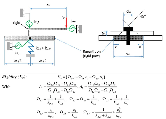
Rotational stiffness
Formula (8) is established for the case where the force is applied at the center of
plate exhibits rotation displacement in addition to the vertical displacement. The
eccentricity of the load is often associated to the eccentricity in the load transfer
from the base plate (in bending) to the repartition plate through the bolts (Fig. 9c
and 9d). Therefore, the rigidity of the system may be modelled by two springs, one
translational (k,c) and one rotational (k,c, see Fig. 12). The translational spring
rigidity (k,c) is given by Eq.(8) while the rotational spring rigidity may be
determined by the following equation:
2 , c R c E w b k (9)
with Ec, the Young modulus of concrete, wR, the width of the rigid plate, b, the
width of the sub-part, , a coefficient defined here after. Eq.(9) is based on the assumption that a full contact between the plate and the concrete is ensured; this
assumption is acceptable as the concrete under the rigid part is normally in
compression on all its area. Physically, the w b2R term in Eq.(9) represents the
flexion modulus of the rigid plate. Again, is determined numerically through the same method used to determine (Eq.(8)); only the compression force is replaced by a bending moment (Fig. 12). From the numerical results, it is observed that the
influence of the Hc/wr ratio is not significant; so this parameter is taken out. Table 4
gives the values of the coefficient which can be used to determine the rigidity of the plate through (Eq.(9)).
2.1.6. Loss of preloading in the bolt
In such joint configuration, a loss of preloading in the bolts may be observed due to
relaxation of the bolts. In the present work, the loss of preloading caused by creep
and shrinkage of the concrete is considered while the relaxation of the bolts is
neglected as it is generally not significant.
The creep phenomenon may be represented by a diminution of the concrete
stiffness according to the time. Using EN-1992, part 1.1 [6] the concrete Young
modulus, Ec(t), at the time t, can be estimated taking into account the creep effect,
from the initial Young modulus (Ec(0)): Ec(t) = Ec(0)(t) where (t) is the creep
coefficient. As the rigidity of the concrete block (Eq.(8)) is directly proportional to
the Young modulus Ec , therefore we can write: k,c(t) = (t)kc(0).
Let us consider a system of concrete and anchor bolt (Fig. 13) at three different
steps: before preloading, just after preloading and at a moment t. At the initial stat
(i.e. before preloading – see Fig. 13), there is no stress in the concrete and the bolt;
the length of the concrete is bigger than the one of the bolt. Just after preloading,
the compression force in the concrete is in equilibrium with the tension force in the
bolt (B(0)), and the length of the concrete block is equal to the length of the bolt. At
time t, due to the decrease of the concrete rigidity, the length of the system
decreases; the compression force in the concrete is still in equilibrium with the
tension force in the bolt but the value is reduced (B(t)). It is easy to obtain the
reduction B to pass from B(0) to B(t) through the following equation:
, , 0 , , 1 (0) 1 1 (0) b c creep b c k k B t B k t k (10)where k,b is the axial rigidity of the bolt given by Eq.(4) while kc,0 is the initial
rigidity of the concrete given by Eq.(8).
Eq.(10) points out that the loss of the preloading due to creep is proportional to the
kb/kc,0 ratio; this remark is useful as it will allow to select an appropriate length and
diameter for the bolt in order to limit the loss of preloading in a reasonable way.
With respect to the shrinkage effect, the deformation of the concrete due to this
phenomenon can be also determined using EN-1992, part 1.1 [6]: shrinkage (t) =
shrinkage(t)Lc where shrinkage(t) is the shrinkage deformation at time t. Therefore, the
loss of the preloading at time t caused by the shrinkage may be calculated by:
, ( )shrinkage b shrinkage
B t k t
(11)
From Eq.(10) and Eq.(11), one obtains the total loss of preload caused by both creep
and shrinkage:
, , 0 , , , 1 (0) 1 ( ) 1 (0) b c b shrinkage b c k k B t B k t k t k (12)From Eq.(12), it can be observed that the two key quantities affecting the loss of
preloading in the bolt are (t) and shrinkage (t). The method to determine these
parameters is available in EN-1992, part 1.1 [6]; they are not given herein. In
references [3] and [4], the procedure to estimate the loss of preloading in anchor bolts
are also presented; however, it seems that the rigidity of the concrete block is
determined from the experimental results, not by the analytical one.
In this section, how to obtain the elastic response of the sub-part from the rigidities of
the individual components given in Section 2.1 is explained. In particular, two
quantities will be determined: the global rigidity of the sub-part and the internal forces
in the bolt (axial force and bending moment). The reasons are that: the rigidity of the
sub-part is required to distribute the loads within the global connection subjected to
moment and axial forces and, the internal forces in the bolts (and in particular the
associated stresses) are required to assess the fatigue behaviour, which regularly leads
to the failure of the bolts if not well assess. The other quantities such as stress in the
base plate or in the tube wall can be easy obtained from the defined ones.
2.2.1. Preliminary information
The following points have to be clarified before assembling the components.
Preloading effect on the concrete + bolts component
Concrete and bolt work together when the preloading effect is still active and they
work separately when the preloading effect is absence (Fig. 14). Therefore, under the
tension force at the base plate, the rigidity of the concrete + the bolt is equal to the sum
of the individual rigidities of the concrete and of the bolt (k,b + k,c) when the
preloading is still present; but the rigidity is equal to the one of the bolt only (k,b) if
the preloading is not present.
Position of the prying force between the base plate and the repartition plate
It is clear that with the bolt preloading, the position of the prying force moves from the
bolt centre to the plate edges, depending on the evolution of the applied force. For the
sake of simplification, only two situations are considered in the calculation: (1) the
farthest position of the prying force when the preloading is present; and (2) the farthest
For the first position, the distance between the bolt and the prying force is
approximated as (Fig. 15):
01 min(2 / 3, 0.52 0.74 )p
e e d t (13)
with e2, the distance between the bolt centre and the base plate edge; d, the bolt
diameter; and tp, the thickness of the base plate. In Eq.(13), “2e2/3” and “0.74tp” terms
are proposed in [1], in this work “0.5d” is added to take into account of the bolt
dimension.
In the case without the preloading, the position of the prying force in a T-stub as
defined in EN-1993, part 1.8 [8] may be applied for the present case (Fig. 15):
02
min( , 1.25 )
2 1e
e
e
(14)Limit point for which the preloading has to be considered or not
As mentioned previously, under the tension load, the sub-part is analysed for two
distinguished situations: with or without bolt preloading. In each case, the evolution of
the internal force in the bolt according to the applied external force can be determined.
The increase of the force in the bolt in the “no preloading” situation is more important
than in the “preloading” situation as illustrated in Fig.16. The intersection point
between the two lines, ((B1, F1) point in Fig. 16), is assumed as the limit to pass from
one situation to another. The detailed values of B1 and F1 will be provided for different
cases in Section 2.2.2. The continuous broken line in Fig.16 represents the considered
evolution of the internal force in the bolt.
Sub-part in compression
It is assumed that the rigidity of the sub-parts in compression is constant and that the
2.2.2. Assembly formulation
From the individual component rigidities given in Section 2.1 and the remarks
reported in Section 2.2.1, the assembly procedure can be defined and carried out. The
results are presented in Tables 5, 6 and 7. In these tables, the mechanical models are
firstly reported and then the formulas that are obtained by analysing the mechanical
models are given. The mechanical models have a level 2 of hyper-staticity, so they can
be easily solved through analytical approaches, as the force method or the
displacement method.
Beside the quantities detailed in Table 5, 6 and 7, other quantities (as forces in the tube
wall or forces in the base plate) can be easily predicted using equilibrium equations.
3. Global connection characterisation
This section aims at providing the procedure to estimate the global behaviour of the
connection. The main objective is to obtain, according to the applied moment (M) and
axial force (N) on the connection:, (1) the global rigidity of the connection; and (2) the
force distribution in each sub-part in tension and compression (from which the elastic
responses of the sub-part may be accordingly deduced) .
The behaviour of the connection under a bending moment and a compression force is
described in Fig. 17. For the sake of simplification, the cross-section of the structures
wall is supposed to remain plane during the loading, therefor the kinematic of the
connection can be controlled by two parameters: position of the neutral axis (given by
the angle in Fig. 17a), and the rotation (represented by in Fig. 17a). The following principles are followed to analyse the system:
The displacement at any point of the connection are written as functions of the angle and the rotation .
With the obtained displacement, using the force-displacement relationship (Fig.17b) one can determine the force in the corresponding sub-part. Meaning
that these forces are also functions of and .
From two equilibrium equations (axial force and bending moment), and can be determined, meaning that all the previously mentioned quantities can be
obtained.
In fact, the expressions become rapidly complicated; so it is not easy to manually solve
the obtained equations. However, it has to be noticed that the behaviour of the
connection can be numerically obtained using quite simple models once the behaviour
of the sub-part is known (Fig.17b). In the numerical model, the sub-parts can be
modelled through 1D “links” with a behaviour law as given in Fig. 17b while the
structure wall may be replaced by “rigid” elements (1D elements can be used).
In this section, the results given in [1] are summarized, the solutions are only valid in
“State A” (Fig.17), i.e. when the preloading effect is still present in the tension zone. The angle can be determined from Eq.(15):
2 1 1 sin / ( ) cossin cos / (sin ( ) cos )
t c w t c K K M Nr K K (15)
In [1] a chart is provide to practically obtain the angle .
3 1 sin 2 ( ) 2 j j w t c t M b r K K K (16)
The tension and compression forces (in the most loaded sub-part) are:
1 (1 cos ) (1 cos ) t t w j c c w j F K r F K r (17)
Finally, the rigidity of the connection is calculated by:
3 1 1 sin 2 ( ) / 2 j w t c t S r K K K b (18)
4. Calculation procedure
For a given connection (geometries and materials) under M and N, the connection may
be analysed using the following procedure to obtain its main properties, as its rigidity,
and the stresses in the bolt.
Step 1: preparation of the data related to the geometry and the materials of the connection
Step 2: Calculation of the rigidities of the individual components
Rotational rigidity of the structure wall (kw): Eq.(2)
Bending rigidity of the base plate (EsI and GsA) and geometry of the base plate
(mainly its effective width determined using Eq.(3))
The axial and rotational rigidities of the bolt: Eqs.(4) and (5). The equivalent rigid part of the repartition plate: Table 2.
Translational and rotational rigidities of the concrete block k,c and k,c: Eqs.(8)
and (9).
Step 3: Calculation of the rigidity in tension and compression of the sub-part
Rigidity in tension: Table 5 for Kt1 and Table 6 for Kt2.
Rigidity in compression, Kc: Table 7.
Step 4: Rigidity of the connection, distribution of the force in the sub-part, force in the bolts
Rigidity of the connection, Sj: Eq.(18)
Force in the sub-part, Ft and Fc: Eq.(17)
Force/or stresses in bolt: Tables 5 and 6.
Some numerical examples to illustrate the above calculation procedure will be
presented in the next section (Section 5).
5. Numerical examples and validation
This section aims at (1) validating the developed models for the sub-part behaviour
proposed in Section 2 through numerical results, and (2) illustrating the design
procedure given in Section 4 (Step 1 to Step 3). In total, six examples are considered,
named Ex 1.1, Ex 1.2, Ex 1.3, Ex 2.1, Ex 2.2 and Ex.3; their geometries are shown in
Fig.18. The same geometries are used for Exs 1.1, 1.2 and 1.3, only the bolt preloading
is different. Also, the same geometries are adopted for Exs 2.1 and 2.2, but the
materials are different. In the numerical models, the actual form of the sub-part, cut
from a cylindrical connection (with rb = 935 mm and rw = 1042.5 mm), is introduced
for Exs 1.1, 1.2 and 1.3, while the rectangular shape is adopted for Exs 2.1, 2.2 and
mm and 32.0 mm are respectively used in the calculations, to take into account of the
threaded portions of the bolt shanks.
The numerical analyses were carried out using LAGAMINE – a non-linear finite
element programme developed at the University of Liège [15]. Elastic materials with
the properties given in Table 8 are introduced; the contacts between the bolt and the
base plate and between the base plate and the repartition plate are also modelled. Fig.
19 shows a general view of the mesh.
In parallel, the proposed analytical procedure is applied for the considered examples.
In Table 8, not only the input data and the main results are reported but also the way
they have been derived in order to illustrate the calculation procedure. Due to the
space limitation, the detail of Ex.3 are not mentioned in Table 8.
The comparison of the rigidities of the sub-parts and the evolution of the forces in the
bolts are presented in Figs. 20 and 21. A good agreement between the numerical and
analytical analyses is observed, in particular for the rigidities under compression. With
respect to the evolution of the forces in the bolts, the analytical method gives
conservative values.
6. Conclusion
A complete analytical model devoted to the characterisation of the elastic behaviour of
bolted connections between cylindrical steel structure and concrete foundation has
been developed. All the required characteristics of the connection (stiffness, stress,
etc.) can be obtained knowning its geometry, the constitutive materials and the applied
external loads. In the proposed model, several parameters have been taken into account
account of the second order effect, the time-dependent properties of the concrete
block, the flexibility characteristics of the base plate and of the repartition plate, etc.
The proposed model is in full agreement with the principle of the component method;
therefore, the proposed model could be easily extended to other types of connections.
The results of the analytical model have been compared with the ones of numerical
models and a good agreement has been observed.
Acknowledgements
This work was carried out with a financial grant from the Research Fund for Coal
and Steel of the European Community, within FRAMEUP project “Optimization of
frames for effective assembling”, Grant N0 RFSR-CT-2011-00035.
References
[1] Couchaux M. Comportement des assemblages par brides circulaires boulonnés (in French) PhD thesis, INSA of Rennes, France, 2010.
[2] Chen W. F., Lui E. M. Stability design of steel structures. CRC Press, 1991.
[3] Delhomme F., Debicki G., Chaib Z. Experimental behaviour of anchor bolts under pullout and relaxation tests. Construction and Building Materials, 24(2010), pp 266-274.
[4] Delhomme F., Debicki G. Numerical modelling of anchor bolts under pullout and relaxation tests. Construction and Building Materials, 24 (2010), pp1232–1238.
[5] EN1090-2. Execution of steel structures and aluminium structures - Part 2: Technical requirements for steel structures. CEN, Brussels, 2008.
[6] EN1992-1-1: Design of concrete structures - Part 1-1: General rules and rules for buildings. CEN, Brussels, 2005.
[7] EN/TS1992-4-1: Design of fastenings for use in concrete - Part 4-1: General. CEN, Brussels, 2009.
[8] EN1993-1-8: Design of steel structures -Part 1.8: Design of joints. CEN, Brussels, 2005. [9] EN1993-1-9: Design of steel structures - Part 1.9: Fatigue. CEN, Brussels, 2005.
[10] EN1993-3-1: Design of steel structures - Part 3-1: Towers, masts and chimneys - Towers and masts. CEN, Brussels, 2006.
[11] EN1993-3-2: Design of steel structures - Part 3-2: Towers, masts and chimneys – Chimneys. CEN, Brussels, 2006.
[12] EN1993-4-1: Design of steel structures - Part 4-1: Silos. CEN, Brussels, 2006.
[13] Guisse S, Vandegans D, Jaspart JP. Application of the component method to column bases – experimentation and development of a mechanical model for characterization. Research Centre of the Belgian Metalworking Industry, 1996.
[14] Jaspart J.P. Recent advances in the field of steel joints – Column bases and further configurations for beam-to-column joints and beam splices. Agregation Thesis, University of Liège, 1997.
[15] LAGAMINE - User’s manual, University of Liege, 2010.
[16] Steenhuis M., Wald F., Stark J. Resistance and stiffness of concrete in compression and base plate in bending. In “Semi-rigid connections in structural steelwork”, Springer Wien New-York, 2000.
[17] Steenhuis M., Wald F., Sokol Z., Stark J. Concrete in compression and base plate in bending. HERON, Vol. 53 (2008), N0 1/2.
[19] Wald F., Bouguin V., Sokol Z., Muzeau J.P. Effective length of T-Stub of RHS column base plates. Czech Technical University, 2000.
[20] Wald F., Sokol Z, Jaspart J.P. Base plate in bending and anchor bolts in tension. HERON, Vol. 53 (2008), N0 2/3.
[21] Wald F., Sokol Z, Steenhuis M., Jaspart J.P. Component method for steel column bases. HERON, Vol. 53 (2008), N0 2/3.
List of Figures
Fig.1. Considered connection Fig.2. Geometries of the sub-part
Fig.3. Rotational rigidity of the tube wall Fig.4. Effective width of the base plate
Fig.5. Effect the nut under the repartition plate
Fig.6. Effect of the direct contact between the bolt and concrete Fig.7. Bolt modelling
Fig.8. Equivalent part of the repartition plate
Fig.9. Determination of rigid part (wr) of the repartition plate
Fig.10. Considered size of the concrete block
Fig.11. Evolution of according to Hc/wr and Lc/wr
Fig.12. Rotational rigidity of the concrete
Fig.13. Deformation of the bolt and concrete due to creep and shrinkage Fig.14. Bolt + concrete component
Fig.15. Position of the prying force
Fig.16. Evolution of the internal force in the bolts Fig.17. Behavior of the global connection
Fig.18. Geometries of the numerical examples Fig.19. Used mesh for the examples
Fig.20. Analytical vs. numerical results (Ex 1.1, 1.2 and 1.3) Fig.21. Analytical vs. numerical results (Ex 2.1, Ex.2.2 and Ex.3)
Fig.2. Geometries of the sub-part
Fig.4. Effective width of the base plate
Fig.6. Effect of the direct contact between the bolt and concrete
Fig.7. Bolt modelling
Fig.9. Determination of rigid part (wr) of the repartition plate
Fig.11. Evolution of according to Hc/wr and Lc/wr
Fig.12. Rotational rigidity of the concrete
Fig.13. Deformation of the bolt and concrete due to creep and shrinkage
0 1 2 3 4 5 6 7 8 1 2 3 4 5 6 7 8 9 C oe ff ic ien t Lc/wr Hc/wr=8 (top) Hc/wr=1 (bottom)
Fig.14. Bolt + concrete component
Ex 1.1- Ex 1.3 Ex 2.1 - Ex 2.2 Ex.3
Fig.18. Geometries of the numerical examples
Ex 1.1 - Ex 1.3 Ex 2.1 - Ex 2.2 Ex.3 Fig.19. Used mesh for the examples
Load (vertical) - Displacement (horizontal) Bolt force (vetical) – Load (horizontal) Analytical results are the continuous lines; Numerical results are the dashed lines; Units: kN, mm
Fig.20. Analytical vs. numerical results (Ex 1.1, 1.2 and 1.3)
-600 -400 -200 0 200 400 600 -0.5 0.5 1.5 2.5 Ex 1.1 0 500 1000 0 100 200 300 Ex1.1 -600 -400 -200 0 200 400 600 -0.5 0.5 1.5 2.5 Ex 1.2 0 400 800 1200 0 200 400 Ex 1.2 -600 -400 -200 0 200 400 600 -0.5 0.5 1.5 2.5 Ex 1.3 0 500 1000 1500 0 200 400 Ex 1.3
Load (vertical) - Displacement (horizontal) Bolt force (vetical) – Load (horizontal) Analytical results are the continuous lines; Numerical results are the dashed lines; Units: kN, mm
Fig.21. Analytical vs. numerical results (Ex 2.1 Ex 2.2 and Ex.3)
-200 -150 -100 -50 0 50 100 150 -0.5 0.5 1.5 2.5 Ex 2.1 0 200 400 600 0 40 80 120 160 Ex 2.1 -600 -400 -200 0 200 400 600 -0.5 0.5 1.5 2.5 Ex 2.2 0 500 1000 1500 2000 0 200 400 Ex 2.2 -200 -100 0 100 200 -0.5 0 0.5 1 1.5 2 2.5 3 Ex.3 0 200 400 600 0 50 100 150 200 Ex.3
List of Tables
Table 1: Stability function values Table 2: determination of wr
Table 3: Coefficient Table 4: Coefficient
Table 5: Analyse of the sub-part under tension with bolt preloading effect Table 6: Analyse of the sub-part under tension without bolt preloading effect Table 7: Analyse of the sub-part under compression
Table 1: Stability function values
Table 2: determination of wr
Cases Formulas
Punctual contact (Figs. 9a and 9b)
2
ca wr 2c
2
ca wr 2a2 Spread contact (Figs. 9c and 9d)
2 b w/ 2 e t d and a2 c wr dw2tb2c 2 b w/ 2 e t d and a2 c wr 2e22c 2 b w/ 2 e t d and a2 c wr dw2tb2a2 2 b w/ 2 e t d and a2 c wr 2e22a2 Table 3: Coefficient Lc/wr 1.0 1.5 2.0 3.0 4.0 5.0 6.0 7.0 8.0 9.0 Hc/wr 1 0.95 0.72 0.66 0.63 0.63 0.63 0.63 0.63 0.63 0.63 2 1.95 1.36 1.16 1.04 1.02 1.02 1.02 1.01 1.01 1.01 3 2.93 2.00 1.65 1.36 1.28 1.25 1.25 1.25 1.25 1.24 4 3.90 2.64 2.14 1.69 1.52 1.45 1.43 1.42 1.42 1.42 5 4.88 3.28 2.63 2.02 1.76 1.64 1.59 1.56 1.55 1.55 6 5.86 3.92 3.12 2.34 2.01 1.84 1.75 1.70 1.68 1.66 7 6.84 4.56 3.61 2.66 2.25 2.04 1.91 1.84 1.80 1.77 8 7.82 5.20 4.10 2.99 2.49 2.23 2.08 1.98 1.92 1.88 Table 4: Coefficient Lc/wr 1.0 1.5 2.0 3.0 4.0 5.95 4.46 4.18 4.03 3.89 klb 0 1 2 3 4 5 6 7 8 9 10 S 4 4.13 4.51 5.08 5.80 6.61 7.48 8.39 9.33 10.29 11.25
Table 5: Analyse of the sub-part under tension with bolt preloading effect Mechanical model Rigidity (Kt1 ):
1 1 1 1 2 2 t FF F F K A A With: 1 2 21 1 22 2 1 12 2 11 12 21 11 22 12 21 11 22 , F F F F A A 1 11 12 21 22 , , , , w 2 3 2 1 1 1 1 1 1 1 2 , , 1 , , 1 1 1 1 1 , , 1 , , 2 3 c b c s c F F FF c s c s s c c e k k k E I k k e e e e e e k E I k E I G A k k Axial force in the bolt: 1 01 1 2 ,
0 01 01 , , b T b c k e e A A B B F e e k k
Maximal bending moment in the bolt:
M
b
F A
T 1 Maximal stress in the bolt:
b
B A
/
b
M W
b/
b Bending moment in the tube wall:M
w
F A
T 2Limit point (Fig.16)
, 1 0 , 1 b c k B B k 1 , 1 01 1 2 1 0 , 01 01 1 b c k e e A A F B k e e Remarks:
kw; k,b; k,c and k,c are given in Eqs.(2), (5), (8) and (9) respectively.
Table 6: Analyse of the sub-part under tension without bolt preloading effect Mechanical model Rigidity (Kt2 )
1 2 1 1 2 2 t FF F F K A A With: 1 2 21 1 22 2 1 12 2 11 12 21 11 22 12 21 11 22 , F F F F A A 02 02 11 2 2 12 21 2 2 02 02 , 02 , ,b 02 02 , 02 , 02 1 02 1 1 02 1 22 1 2 2 1 2 2 02 02 , 02 , w 02 02 , 02 , 2 1 1 1 1 1 1 1 , 3 3 1 1 1 1 1 , 3 3 1 s s b c s s b c F s s b c s s b c F s e e E I G Ae e k e k k E I G Ae e k e k e e e e e e e e E I G Ae e k e k k E I G Ae e k e k e E I 1 02 12 1 1 02 1 2 2 02 02 , 0 , 2 3 2 2 2 1 02 1 1 1 02 1 1 2 2 02 02 02 , 1 3 2 ( ) 1 1 3 s b c FF s s b c e e e e e e G A e e k e k e e e e e e e e E I G A e e k e k Axial force in the bolt: 1 02 1 2
1 1 02 02 ( T ) e e A A B B F F e e
Maximal bending moment in the bolt:
M
b
F A
T 1Maximal stress in the bolt:
b
B A
/
b
M W
b/
b Bending moment in the tube wall:M
w
F A
T 2Remarks:
kw; k,b; k,b and k,c are given in Eqs.(2), (4), (5) and (8) respectively
F1 is given in Table 5.
Table 7: Analyse of the sub-part under compression Mechanical model Rigidity (Kc):
1 1 1 2 2 c FF F F K A A With: 1 2 21 1 22 2 1 12 2 11 12 21 11 22 12 21 11 22 , F F F F A A 11 12 21 22 , ,b , , w 2 1 1 1 1 2 , , , , , 1 1 1 1 1 , , 1 , , c c c F F FF c c c b c k k k k k e e e k k k k k Remarks:kw; k,b;k,b; k,c and k,c are given in Eqs.(2), (4), (5), (8) and (9) respectively
Table 8: input data and results given by the analytical method
Quantities Ẽxamples
Symb ol
Reference Unit Ex.1.1 Ex.1.2 Ex.1.3 Ex.2.1 Ex.2.2
(1) (*) (2) (*) (3) (*) (1) (*) (2) (*) (3) (*) (1) (*) (2) (*) (3) (*) (1) (*) (2) (*) (3) (*) (1) (*) (2) (*) (3) (*)
Material, geometries and preloading (the same geometry (Fig.1) for Ex. 1.1 , Ex.1.2 and Ex.1.3; the same geometry (Fig.1) for Ex.2.1 and Ex.2.2)
E Young modulus kN/mm2 210.0 210.0 1680.0 Eb kN/mm2 210.0 210.0 630.0 Ec kN/mm2 31.0 31.0 31.0 rb Geometries (Figs.1 & 18) mm 935 - b(**) mm 140.6 120.0 tb mm 64.0 30.0 tp mm 40.0 50.0 tw mm 15.0 - rw mm 1042.5 - lb mm 743.0 680.0 d mm 46.5 27.0 dw mm 78.0 56.0 Hc mm 639.0 600.0 e1 mm 107.5 12.0 e2 mm 78.0 12.0 B0 Preloading kN 460.0 460.0 460.0 670.0 670.0 670.0 950.0 950.0 950.0 405.0 405.0 405.0 1060.0 1060.0 1060.0 Intermediate quantities e01 Eq.(13) mm 47.36 - - 47.36 - - 47.36 - - 35.7 - - 35.7 - - e02 Eq.(14) - 78 - - 78 - - 78 - - 120 - - 120 - beff Eq.(3) mm 119.51 119.51 119.51 119.51 119.51 119.51 119.51 119.51 119.51 102 102 102 102 102 102 wr Table 2 mm 256 10 256 256 10 256 256 10 256 241 80 241 320 80 320 Lc (***) mm 476 320 476 476 320 476 476 320 476 520 280 520 520 280 520 Table 3 - 1.49 2.46 1.49 1.49 2.46 1.49 1.49 2.46 1.49 1.37 2.60 1.37 1.23 2.60 1.23 Table 4 - 4.27 - 4.27 4.27 - 4.27 4.27 - 4.27 4.15 - 4.15 4.39 - 4.39 e1 Figs. 1 & 18 mm - - 107.5 - - 107.5 - - 107.5 - - 120 - - 120 ex Fig.18 mm - - 12.5 - - 12.5 - - 12.5 - - 0.00 - - 0.00 S Eq.(6) - 4.66 4.66 4.66 4.93 4.93 4.93 5.28 5.28 5.28 7.35 7.35 7.35 7.00 7.00 7.00 kw Eq.(2) kNm 18.76 18.76 18.76 18.76 18.76 18.76 18.76 18.76 18.76 - - - - k,b Eq.(4) kN/mm 479.74 479.74 479.74 479.74 479.74 479.74 479.74 479.74 479.74 176.73 176.73 176.73 530.19 530.19 530.19 k,b Eq.(5) kNm 30.21 30.21 30.21 32.00 32.00 32.00 34.25 34.25 34.25 5.92 5.92 5.92 16.93 16.93 16.93 k,c Eq.(8) kN/mm 2925.2 1771.8 2925.2 2925.2 1771.8 2925.2 2925.2 1771.8 2925.2 2715.3 1430.8 2715.3 3017.0 1430.8 3017.0 k,c Eq.(9) kNm 6689.6 - 6689.6 6689.6 - 6689.6 6689.6 - 6689.6 5206.3 - 5206.0 8677.2 - 8673.2
Final results (the global rigidities (Kt or Kc), point (B1, F1) from which the effect of the preloading is considered as absence (Fig. 16))
Kt (Kc) Tables 5-7 kN/mm 730.79 84.95 2150.2 730.81 85.48 2149.9 730.84 86.15 2150.2 76.58 21.77 1607.6 499.46 90.58 2233.7
B1 Table 5 kN 535.44 - - 779.88 - - 1105.8 - - 431.36 - - 1246.3 - -
F1 Table 5 kN 164.25 - - 239.28 - - 339.36 - - 98.99 - - 286.18 - -
(*): (1) = in tension with preloading; (2) = in tension without preloading; and (3) = in compression (always with preloading) (**): for Ex 1.1, 1.2 and 1.3, b is calculated using Eq.(1), while b is obtained using Fig.18. for Ex 2.1., 2.2.