SEISMIC VULNERABILITY ASSESSMENT OF
SCHOOLS DESIGNATED AS POST-DISASTER
SHELTERS IN MONTRÉAL
by
Ghaleb DAMAJ
THESIS PRESENTED TO ÉCOLE DE TECHNOLOGIE SUPÉRIEURE
IN PARTIAL FULFILLMENT FOR A MASTER’S DEGREE
WITH THESIS IN CONSTRUCTION ENGINEERING
M.A.Sc
MONTRÉAL, JULY 15, 2020
ÉCOLE DE TECHNOLOGIE SUPÉRIEURE
UNIVERSITÉ DU QUÉBEC
This Creative Commons license allows readers to download this work and share it with others as long as the author is credited. The content of this work cannot be modified in any way or used commercially.
BOARD OF EXAMINERS
THIS THESIS HAS BEEN EVALUATED BY THE FOLLOWING BOARD OF EXAMINERS
Rola Assi, Thesis Supervisor
Department of Construction Engineering, École de technologie supérieure
Ghyslaine McClure, Thesis Co-supervisor
Department of Civil Engineering and Applied Mechanics, McGill University
Richard Arsenault, President of the Board of Examiners
Department of Construction Engineering, École de technologie supérieure
Ahmad Abo El Ezz, Member of the jury
Scientific researcher, Geological Survey of Canada, Natural Resources Canada
THIS THESIS WAS PRENSENTED AND DEFENDED IN THE PRESENCE OF A BOARD OF EXAMINERS
JUNE 22, 2020
ACKNOWLEDGMENT
I would like to express the deepest appreciation to my supervisor, Professor Rola Assi (ÉTS) and my co-supervisor Professor Ghyslaine McClure (McGill University) for their guidance and encouragement. The completion of this work could not have been possible without their participation and assistance. I am extremely grateful to them for providing such a nice support which made me complete this project.
I would like to acknowledge the financial support of Professor Rola Assi and the Centre d’études interuniversitaire des structures sous charges extrêmes (CEISCE).
Finally, I would like to thank my family, for their enduring support and their help, either directly or indirectly with my graduate studies.
Évaluation de la vulnérabilité sismique des écoles désignées comme des abris d’urgence à Montréal
Ghaleb DAMAJ
RÉSUMÉ
Ce projet vise à évaluer le risque sismique associé aux composants non structuraux (CNS) – aussi connus au Canada sous le nom de composants fonctionnels et opérationnels (CFO), dans 16 écoles désignées comme des abris post-catastrophe à Montréal par le Centre de sécurité civile de Montréal. Un indice déterministe amélioré de vulnérabilité structurale (VI) est déterminé par le processus d’analyse hiérarchique (PAH) en tenant compte des principaux paramètres structuraux considérés lors d’une étude précédente réalisée à l’Université McGill. L’étude précédente était réalisée sur la base d’inspection visuelle des bâtiments adaptée de la méthode américaine FEMA 154 (Federal Emergency Management Agency) et de la norme de conception parasismique des bâtiments de Nouvelle-Zélande. Les principaux paramètres considérés sont le type de système de résistance aux charges latérales, la hauteur du bâtiment, son année de construction, la présence d’irrégularités structurales (verticales et horizontales), ainsi que la sismicité et la classe de sol du site local définies dans le code national du bâtiment du Canada (CNB). La méthode PAH est appliquée pour estimer un facteur de pondération pour chacun des paramètres affectant la vulnérabilité sismique du bâtiment via une comparaison par paire de leur contribution afin d’améliorer l’équation de la vulnérabilité structurale proposée dans la norme CSA S832- Réduction du risque sismique associé à la défaillance des composants fonctionnels et opérationnels des bâtiments. Les résultats du nouvel indice de vulnérabilité ont été calibrés avec les résultats d’une étude précédente entreprise à l’Université McGill. Cette étape est suivie par l'intégration de l'effet de la résonance sol-superstructure en tant que nouveau paramètre dans l'évaluation de la vulnérabilité structurale à l'aide de la méthode PAH. Le nouveau VI est également classifié selon une échelle révisée qui contient quatre niveaux d’intensité : faible, modéré, élevé et très élevé. L’ajout du paramètre de résonance a augmenté la classe de vulnérabilité sismique dans certains cas. Enfin, le risque sismique associé aux CFO est évalué selon la norme CSA S832 en utilisant le VI amélioré. Conformément à cette norme, le risque sismique est évalué par le calcul d’un indice de risque (R) tenant en compte la vulnérabilité du bâtiment, l’aléa sismique du site, la vulnérabilité du composant en fonction de son mode d’attache à la structure, la possibilité de choc, martelage et renversement du CFO, sa flexibilité et son emplacement dans le bâtiment, ainsi que les conséquences liées à la rupture ou la non-fonctionnalité du CFO. Les résultats de l’indice de risque sont classifiés selon la même échelle que celle du CSA S832.
Mots-clés: Risque sismique, PAH, résonance sol-structure, indice de vulnérabilité, CFO,
Seismic vulnerability assessment of schools designated as post-disaster shelters in Montréal
Ghaleb DAMAJ
ABSTRACT
This research aims to assess the seismic risk associated to the non-structural components (NSCs), also known in Canada as operational and functional components (OFCs), of 16 schools designated as post-disaster shelters in Montréal by the Civil Safety Department of the City of Montréal. An improved deterministic structural vulnerability index (VI) is calculated using the Analytical Hierarchy Process (AHP). The new VI considers the main structural parameters considered in a previous study conducted at McGill University using the seismic screening method adapted from the American FEMA 154 (Federal Emergency Management Agency) and New Zealand guidelines. The main parameters include the type of lateral load resisting system, the building height, the year of construction, the presence of structural irregularities (vertical and horizontal), as well as the seismicity and soil class at the site as prescribed by the seismic design provisions of the National Building Code of Canada (NBC). The AHP method is applied to estimate a weight factor for each parameter contributing in the structural vulnerability via a pairwise comparison, in order to develop an improved structural vulnerability equation. The new vulnerability index is calibrated with the results of the previous study at McGill University. This calibration is followed by the integration of the effect of soil-building resonance as a new parameter in the assessment of the structural vulnerability currently proposed in the CSA S832 standard (Seismic risk reduction of operational and functional components). The new VI is classified into four categories: low, moderate, high and very high. The addition of the soil-building resonance parameter has increased the building seismic structural vulnerability classes in some cases. Finally, the seismic risk associated to the OFCs is assessed based on the improved structural vulnerability index and the CSA S832 parametric method based on onsite inspection. Accordingly, the evaluation of the seismic risk is represented by calculating a risk index (R) that takes into consideration the vulnerability of the building, the seismic hazard at the building site and the vulnerability of the component based on the OFC restraint, impact and pounding, OFC overturning and OFC flexibility and location in building, in addition to the consequences of OFC failure or lack of functionality. The risk indices are classified according to the mitigation priority thresholds of CSA S832.
Keywords: Seismic risk, AHP, soil-building resonance, seismic screening method, OFC,
TABLE OF CONTENTS
Page
INTRODUCTION ...1
CHAPTER 1 LITERATURE REVIEW ...5
1.1 Seismic performance of school buildings and their OFCs during past high magnitude earthquakes ...5
1.2 Seismic vulnerability and assessment methods ...6
1.2.1 Quantitative assessment methods ... 9
1.2.2 Qualitative assessment methods ... 21
1.3 Previous studies on post-earthquake functionality of buildings ...36
1.4 Previous studies on the effects of soil-structure resonance ...39
1.5 Analytical Hierarchy Process (AHP) ...41
CHAPTER 2 SEISMIC STRUCTURAL VULNERABILITY OF SCHOOLS IN MONTRÉAL CONSIDERING THE EFFECT OF SOIL-BUILDING RESONANCE ...46
2.1 School building databases ...47
2.2 Reliability of the ambient vibration measurement test results ...48
2.3 Coefficient of soil-building resonance ...49
2.4 Vulnerability index from AHP...51
2.5 Validation of vulnerability index using AHP ...53
2.6 Limitations ...57
CHAPTER 3 NEW OFC SEISMIC RISK INDEX ACCORDING TO THE CSA S832 METHOD ...58
3.1 Setting building vulnerability index limits ...58
3.2 Improvement of the OFC seismic risk index with effect of the variation of the local seismicity ...59
3.3 New OFC seismic risk index for a case study building in Montréal ...60
3.3.1 Drift-sensitive components ... 61
3.3.2 Acceleration-sensitive components ... 64
3.4 Effect of the seismicity on the OFC seismic risk ...66
3.5 Observations ...70
CHAPTER 4 SUMMARY AND CONCLUSIONS ...71
4.1 New seismic structural vulnerability index ...71
4.2 New OFC seismic risk index ...72
4.3 Conclusions ...72
4.4 Suggestions for future work ...74
APPENDIX II DYNAMIC PROPERTIES OF THE STUDIED BUILDINGS AND THE ADJACENT SOIL ...86 APPENDIX III VALIDATION OF THE AHP RESULTS WITH THE ADAPTED
SEISMIC SCREENING METHOD ...91 APPENDIX IV DETAILED APPLICATION OF THE AHP-BASED METHOD AND
THE ADAPTED SCREENING METHOD ...99 LIST OF BIBLIOGRAPHICAL REFERENCES ...101
LIST OF TABLES
Page
Table 1.1 Types of Lateral Load Resisting Systems according to FEMA 154 ...24
Table 1.2 Collapse rates by model building type for complete structural damage ...25
Table 1.3 Basic score and score modifiers according to Tischer’s adapted screening method...26
Table 1.4 Basic score and score modifiers according to Tischer’s adapted screening method...27
Table 1.5 Seismic vulnerability ranking system used in Oregon with FEMA 154 ...28
Table 1.6 Damage functions for seismic screening in Eastern Canada ...28
Table 1.7 Ground motion amplification factors for Montréal, according to NBC 2015...29
Table 1.8 Building characteristics index according to CSA S832-14 ...32
Table 1.9 Individual OFC parameters and weight factors according to CSA S832-14 ...33
Table 1.10 Rating scores for OFC characteristic index according to CSA S832-14 ..34
Table 1.11 Rating scores used for the determination of the consequence index of OFCs according to CSA S832-14 ...35
Table 1.12 Suggested mitigation priority thresholds according to CSA S832-14 ...36
Table 1.13 AHP scale of preference between two parameters ...42
Table 2.1 Priority and normalized weights of five parameters from the adapted screening method according to AHP ...52 Table 2.2 Priority and normalized weights of five parameters including the
coefficient of resonance according to AHP ...52 Table 2.3 Structural vulnerability classes according to the proposed method ...53 Table 2.4 Characteristics of eight concrete buildings (School 16 in Appendix I) ...54 Table 2.5 Comparison of structural vulnerability indices and classes according to
the AHP-based method and Tischer’s adapted screening method without the coefficient of resonance ...54 Table 2.6 Comparison of structural vulnerability index and class according to the
AHP-based method with consideration of the coefficient of soil-building resonance for a school campus with 8 buildings ...55 Table 2.7 Comparison of Structural vulnerability index and class according to the
AHP-based method considering soil-building resonance and Tischer’s adapted screening method for two buildings (School 1 in Appendix I) ....56 Table 2.8 Comparison of the vulnerability class according to the AHP-based
method considering soil-building resonance and Tischer’s adapted
screening for a school campus of 6 buildings (School 6 in Appendix I) ...56 Table 3.1 Characteristics of the case study school building (School 16 in Appendix
I). ...60 Table 3.2 Drift-sensitive components located in Building T ...62 Table 3.3 Comparison of the improved seismic risk index of the critical
drift-sensitive components with the existing risk according to CSA S832 ...63 Table 3.4 Suggested mitigation priority thresholds according to CSA S832 ...64
Table 3.5 Critical acceleration-sensitive components located in Building T ...65 Table 3.6 Comparison of the improved seismic risk index of the critical
acceleration-sensitive components. ...65 Table 3.7 Improved seismic risk index, R, for drift-sensitive components with
different seismicity...67 Table 3.8 Seismic risk index, R, according to CSA S832 for drift-sensitive
components with different seismicity ...68 Table 3.9 Improved seismic risk index, R, for acceleration-sensitive components
with different seismicity ...69 Table 3.10 Seismic risk index, R, according to CSA S832 for acceleration-sensitive
LIST OF FIGURES
Page
Figure 1.1 Operational and Functional Components (OFCs) in buildings ...7
Figure 1.2 Relative direct costs of building components according to use and occupancy ...8
Figure 1.3 Nonlinear static analysis procedure ...10
Figure 1.4 Schematic of Static Pushover Analysis used in the Capacity Spectrum Method ...11
Figure 1.5 Graphical representation of the capacity spectrum method ...11
Figure 1.6 Flow Chart of NDA to Determine Seismic Building Response ...13
Figure 1.7 Main steps of FRACAS for the derivation of the performance point (PP) using the trilinear idealization model ...15
Figure 1.8 Flowchart of the FaMIVE procedure ...17
Figure 1.9 Modules of HAZUS ...19
Figure 1.10 Fragility curves for slight, moderate, extensive and complete damage ...20
Figure 1.11 Example of a building capacity curve ...21
Figure 1.12 Analysis procedure in the building portfolio recovery model (BPRM) ....37
Figure 1.13 Flowchart of the probabilistic approach of pre-recovery damage and functionality loss assessment ...37
Figure 1.14 Building damage and utility availability to building functionality states ..38
Figure 2.1 Distribution of LLRS for the evaluated schools using the adapted seismic screening method ...47 Figure 2.2 Tromino sensor ...48 Figure 2.3 Average fundamental frequency of the tested soil site ...49 Figure 2.4 Distribution of coefficients of soil-building resonance for 69 buildings
LIST OF ABBREVIATIONS
ADRS Acceleration-displacement response spectrum AHP Analytical hierarchy process
ATC Applied Technology Council (United States) AVM Ambient vibration measurement
BHRC Building housing research center (United States) BPRM Building portfolio recovery model
BSH Basic structural hazard CMF Concrete moment frame
CIW Concrete frame with infill masonry shear walls
CR Consistency ratio
CoR Coefficient of resonance
CSM Capacity spectrum method
CSW Concrete shear walls DOF Degree of freedom
FaMIVE Failure mechanism identification and vulnerability evaluation FEMA Federal Emergency Management Agency (United States) FRACAS Fragility through capacity spectrum method
GIS Geographic information system HAZUS Hazard United States Software
HVMWR Horizontal-to-vertical moving window ratio HVSR Horizontal-to-vertical spectral ratio
LLRS Lateral load resisting system
MCE Maximum considered earthquake NASW Noise analysis of surface waves
NBC National Building Code of Canada NDA Nonlinear dynamic analysis
NRC National Research Council of Canada
NSC Nonstructural component
OFC Operational and functional component
PCF Precast concrete frame
PCW Precast concrete walls
PESH Potential earth science hazards PGA Peak ground acceleration RI Random consistency index
RMC Reinforced masonry bearing walls with concrete diaphragm
RML Reinforced masonry bearing walls with wood and metal deck floors SBF Steel braced frame
SCW Steel frame with concrete shear walls SDOF Single degree of freedom
SIW Steel frame with infill masonry shear walls
SLF Steel light frame
SM Score modifiers
SMF Steel moment frame
SPI Seismic priority index
STD Standard deviation
STFT Short time Fourier transform
URM Unreinforced masonry bearing walls
VI Vulnerability index
WLF Wood light frame
WPB Wood post-and-beam construction
LIST OF SYMBOLS
A Standard pseudo acceleration
C Consequence score
D Deformation spectrum ordinate V Vulnerability
R Risk index
βeq Equivalent viscous damping ratio Γ Modal participation factor
Fa Soil modification factor in NBC F0 Seismic force at OFC
M1 Effective modal mass
Sa Spectral acceleration
Sa (0.2) Spectral acceleration at 0.2s
SD Spectral displacement
Teq Equivalent fundamental period
Tn Natural period
Vb Base shear
Vs30 Site shear wave velocity averaged over 30-m depth t0 Time of occurrence of scenario
VB Building characteristics index VE OFC characteristics index
VG Ground motion characteristics vulnerability index Vtotal Total lateral load
µN Top floor displacement φ Mode shape vector Meff Tributary mass
Keff Lateral effective stiffness
INTRODUCTION
Previous studies and experience from past earthquakes have demonstrated that there is a need to assess the seismic vulnerability of school buildings even in zones of moderate seismicity (Dolce, 2004). One may recall the adverse performance of schools during the Mw 8.0 Sichuan (China) earthquake in 2008 that resulted in the deaths of hundreds of children while at school (Revkin, 2008). Although such severe earthquakes are not likely in Québec, school buildings remain potentially vulnerable to moderate shaking as many may have inadequate exit pathways, and students/pupils may not be able to exit safely and quickly enough when an emergency occurs (Rodgers, 2012). In Québec, most school buildings have structural irregularities, and many would likely have poor seismic performance if subjected to moderate to strong earthquakes because they were designed and built in the 1960s and 1970s, before the introduction of modern earthquake-resistant design procedures in the National Building Code of Canada (NBC). Another compelling reason to assess their seismic vulnerability is that school buildings (secondary school buildings in particular) are possible candidates to serve as post-critical shelters in case of disasters. Therefore, school buildings must remain structurally safe at all times (Chakos, 2004), hence the importance of adequately assessing their seismic vulnerability and post-earthquake functionality.
The present research contributes to a better assessment of seismic structural vulnerability and post-earthquake functionality of 16 schools designated as post-disaster shelters in Montréal by introducing the soil-building resonance as a parameter deemed to affect their vulnerability. The Analytical Hierarchy Process (AHP) is used to integrate this resonance parameter in the seismic structural vulnerability assessment of buildings, and to calibrate it with the adapted seismic screening method developed by Tischer (Tischer, 2012). Furthermore, the assessment of the seismic risk associated to the operational and functional components (OFCs) located in the schools is conducted by applying the method proposed in the CSA S832 standard (CSA, 2014) with an improved building structural vulnerability index,VB, that considers soil-building resonance effects and structural irregularities.
Objective
The main objective of this study is to propose an improved method for assessing the post-earthquake functionality of school buildings designated as post-disaster shelters in Montréal. The post-earthquake functionality of a building depends both on its structural integrity and safety and on the integrity of its OFCs. The study recommends improving the parametric method proposed in CSA S832 for seismic risk assessment of OFCs by considering new parameters associated with structural irregularities of the lateral-load resisting system of the building, the year of construction, and the possible soil-building resonance effect. To account for the latter, a coefficient of resonance (CoR) is calculated and added to the evaluation of the building vulnerability index (VB) using the AHP method.
Methodology
To achieve the main research objective, the applied methodology comprises the following steps:
1) Study of the existing information on school buildings designated as post-disaster shelters in Montréal, which forms the database of the current study.
2) Evaluation of the adapted seismic screening method proposed by Tischer (2012) and inspired by the rapid visual screening of buildings for potential seismic hazard (FEMA 154).
3) Extraction of the dynamic properties of 69 school buildings and local soil, such as the fundamental frequency and damping ratio of the structures.
4) Estimation of the coefficient of soil-building resonance by dividing the fundamental frequency of the adjacent soil by the fundamental frequency of the school building. The school buildings having a coefficient of resonance between 0.9 and 1.1 are classified as vulnerable to resonance.
5) Development of new vulnerability index using AHP, in order to evaluate the seismic structural vulnerability of schools considering possible soil-building resonance.
6) Estimation of a new OFC seismic risk index based on the CSA S832 parametric method using the new proposed structural vulnerability index.
Organization of the report
This report consists of four chapters. Chapter 1 provides background and a brief literature review of the performance of school buildings during past earthquakes and the previous methods used to assess the seismic structural and non-structural vulnerabilities as well as the effect of soil-building resonance on the seismic vulnerability. Chapter 2 presents the development of a new structural vulnerability index that considers the effect of soil-building resonance by applying the AHP method. Chapter 3 describes the estimation of the new seismic risk index based on the CSA S832 method and the application of the AHP method.
Finally, Chapter 4 states the original contributions of the current study as well as its impact and limitations and some recommendations for future work.
CHAPTER 1 LITERATURE REVIEW
The performance of school buildings during past earthquakes is reviewed next. In addition, this chapter presents the available rapid screening methods to assess seismic structural and non-structural vulnerabilities. The description of the adapted seismic screening method developed by Tischer (Tischer, 2012) and the CSA S832 (CSA, 2014) parametric method are reviewed in more detail as well as the theory of the Analytical Hierarchy Process (AHP).
1.1 Seismic performance of school buildings and their OFCs during past high magnitude earthquakes
The poor seismic performance of school buildings in many countries has made their vulnerability assessment and retrofit a priority in moderate and high seismic zones. According to the Building and Housing Research Center of the United States (BHRC, 2005), school buildings are considered as vital structures, so upgrading them to sustain the effects of strong earthquakes is highly important to reduce loss of life. The good seismic performance of OFCs is essential to ensure the building safety and functionality, especially in school buildings designated as post-disaster shelters.
The recent September 2017, Mw 7.1 earthquake in Mexico City has killed 22 people at a school that collapsed (Singh et al., 2018). In eastern Turkey, the city of Van has been hit by a Mw 7.1 earthquake on October 23, 2011, which caused the collapse of 58 buildings, including some schools, and 604 human deaths and more than 2000 injured (222 of them were rescued under the collapsed buildings) (Taskin et al., 2013) . Moreover, during the February 2010, Mw 8.8 earthquake in Chile, around 2000 schools were heavily damaged (Ghosh & Cleland, 2012). In Pakistan, the Mw 7.8 earthquake that hit Kashmir on October 8, 2005, has badly affected the three main districts facilities such as hospitals, schools and services including police and armed forces (Peiris et al., 2008). The earthquake occurred during day school time hours, with resulted in the tragic death of approximately 19000 pupils and students, most of them trapped
under the collapsed school buildings. Another example is the catastrophic Mw 9.3 earthquake and tsunami that struck Indonesia in 2004 and destroyed approximately 750 school buildings and damaged more than 2000 other, killing thousands of teachers and students (McAdoo et al., 2006). Built in 1960, the Iovene primary school in San Guiliano, Italy collapsed during the more moderate October 31, 2002 Mw 5.5 Molise earthquake, causing approximately 28 children deaths (Decanini et al., 2004). The amplification of the ground motion from the local soil conditions and poor unreinforced masonry construction have caused the collapse (Dolce, 2004). The 20 October 1999 Mw 7.6 earthquake that hit Chi-Chi in Taiwan caused the collapse of 51 schools while many other school buildings experienced considerable damage (Kelson et al., 2001). Moreover, the July 1997, Mw 6.8 earthquake in Caraico, Venezuela destroyed four school buildings; most of them were concrete frames with unreinforced infill masonry, and they collapsed due to their weak resistance and stiffness (López et al., 2007). To mention a few Canadian examples, the relatively moderate 1988 Mw 5.9 Saguenay earthquake caused architectural damage that cost several millions of Canadian dollars in repair and retrofit (Tinawi & Mitchell, 1990). A total of 16 of the 25 schools of the Chicoutimi public school board experienced severe architectural damage that cost around 3 million dollars to repair, and 17 schools of the Baie des Ha! Ha! School board also suffered severe architectural damage that cost 2.8 million dollars.
1.2 Seismic vulnerability and assessment methods
The seismic vulnerability of a building structure and its non-structural components is defined by their inability to resist the effects of earthquake-induced forces and displacements, thus jeopardizing life safety and building functionality. It is a global concept that can be sub-divided into seismic structural vulnerability (addressing life safety) and seismic vulnerability of its OFCs (addressing building functionality). The seismic vulnerability level can be evaluated and expressed by functions that can be derived either by statistical studies of damaged buildings in earthquakes or by simulations using analytical, probabilistic and numerical methods (Calvi et al., 2006).
Figure 1.1 shows typical building OFCs that are permanently or temporarily attached to the structure so that their seismic vulnerability is strongly affected by the quality and configuration of their anchoring to the supporting structure.
Figure 1.1 Operational and Functional Components (OFCs) in buildings (Source: CSA S832-14 (2014))
Taghavi and Miranda (2003) noted that damage to OFCs yields the largest economic losses due to earthquakes; the cost of these components typically represents 60% to 90 % of the total construction cost for buildings with intended use and occupancy of office/schools, hotels and hospitals, as illustrated in Figure 1.2. In addition to the costs caused by direct damage to the components themselves, further losses are suffered as the building functionality is compromised, even if the structure is safe. The level of vulnerability of OFCs can be high if their restraints are inadequate and the OFCs are prone to instability that might cause
overturning and/or sliding. According to the parametric method of CSA S832 (CSA, 2014), the vulnerability index of OFCs depends on their location in the building and their connection with the structure, such as anchorage configuration and load path. The higher the vulnerability of these components, the higher the seismic risk, which is a function of the vulnerability and consequences. Overall, the risk is related to threats to life safety, loss of function and property loss. Moreover, the vulnerability of OFCs has direct consequences on the safe evacuation of buildings.
Figure 1.2 Relative direct costs of building components according to use and occupancy (Source: Taghabi & Miranda (2003))
Losses due to OFC damage can range from minor to severe depending on their use and replacement cost. For example, if the bookshelves in school libraries are not properly secured and restrained, they can topple without having a significant loss of function (or material losses), but they are a human life hazard if the premises are occupied during the earthquake.
Bertogg et al. (2002) noted that the loss analysis must focus at least on the basic vulnerability parameters that can be used in a typical risk model. It is extremely important to distinguish
between the more detailed assessment of individual buildings and the assessment of groups of buildings at the so-called urban scale (Vicente et al., 2011).
A description of the basic principles of the most common quantitative assessment methods follows, including the capacity spectrum method (CSM), the fragility through capacity spectrum method (FRACAS), the failure mechanism identification and vulnerability evaluation (FaMIVE), the methodology of HAZUS, and the probabilistic post-earthquake functionality assessment method. It is followed by a more detailed description of the qualitative assessment methods prescribed in Canada such as the rapid screening National Research Council (NRC 1992) method and the parametric seismic risk assessment method of CSA S832 (CSA, 2014) for OFCs.
1.2.1 Quantitative assessment methods
1.2.1.1 CSM (Capacity spectrum method) and the use of nonlinear analysis
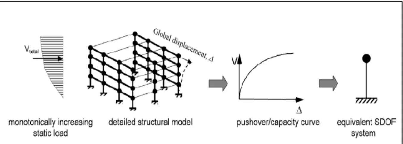
The capacity spectrum method (CSM) is a performance-based seismic analysis method that can be used for many purposes such as the rapid evaluation of a large number of building structures. It is one of the most commonly used procedures to assess the building behaviour during an earthquake. It is essentially a nonlinear static pushover analysis procedure formally developed by Freeman (Freeman, 1998) but its original concept was introduced for seismic evaluations in the ATC-40 (ATC, 1996) as shown in Figure 1.3 to Figure 1.5. This method includes the following steps: (a) development of pushover curve, (b) conversion of pushover curve to capacity diagram, (c) conversion of elastic response spectrum from standard format to A-D format, and (d) determination of displacement demand. (A: standard pseudo-acceleration, D: Deformation spectrum ordinate).
Figure 1.3 Nonlinear static analysis procedure (Source: ATC (1996))
As shown in Figure 1.3, uN is the top floor displacement, φΝ1 is the fundamental mode shape ordinate at the top floor, Vb is the base shear and Γ is the modal participation factor and M1 is the effective modal mass for the fundamental vibration mode. The Vtotal shoin Figure 1.4 is the total lateral load and Δ is the global displacement.
Figure 1.4 Schematic of Static Pushover Analysis used in the Capacity Spectrum Method (Source: ATC (2005))
Figure 1.5 Graphical representation of the capacity spectrum method (Source: ATC (2005))
As shown in Figure 1.5, the seismic demand in acceleration, Sa, and relative displacement, Sd, of an equivalent single degree-of-freedom system is represented by a response spectrum (curves in red) and the structural capacity is represented by the pushover curve (in green). This format is called the acceleration-displacement response spectrum (ADRS). The expected performance of the structure, called the performance point, is the intersection point of the seismic demand and capacity spectrum curves. To account for the nonlinear inelastic behavior of the building, a viscous damping ratio β is introduced. Therefore, each building type is modeled as a nonlinear single-degree-of-freedom (SDOF) for which the maximum inelastic deformation is calculated based on the maximum elastic deformation of an equivalent linear elastic SDOF with equivalent fundamental period (Teq) and viscous damping ratio (βeq). Where β0 shown in Figure 1.6 represents the initial damping value and βeq is referred to as effective viscous damping. The equivalent fundamental period and damping ratio are determined from the seismic demand and capacity curves for a given lateral load resisting system. As mentioned above, the capacity curve is the lateral force-deformation relationship for a given structure obtained from pushover analysis. Therefore, the fundamental period corresponding to the point of intersection of the demand curve and the capacity curve is considered as the equivalent period of the linear SDOF oscillator. The equivalent viscous damping is estimated from the energy dissipated in a vibration cycle of the inelastic system and the equivalent linear system. The estimated spectral displacement is then used to determine the cumulative probability of complete damage from the fragility curves specific to the building type.
In addition to this nonlinear static analysis approach, there is a more exact nonlinear dynamic analysis (NDA) method. In this method, the first step is to create a finite element model of the building structure to capture its nonlinear post-elastic response under ground motions, as shown in Figure 1.6. NDA allows higher modes of vibration to be captured as well as different failure modes, which is not properly done in the ADRS format. Of course, the quality of the NDA method depends directly on the accuracy of the analysis model created to represent the real building.
Figure 1.6 Flow Chart of NDA to Determine Seismic Building Response (Source: ATC (2005))
The nonlinear dynamic procedure is used to represent the seismic response of buildings to several different ground motions for different earthquakes corresponding to tectonic models appropriate for the building location. NDA permits to obtain not only the mean response to a specific ground motion, but it also allows to account for the nonlinear response of buildings generated by different records for the same earthquake intensity measure (Jalayer & Cornell, 2009) (Vamvatsikos & Cornell, 2005), while the linear dynamic procedure ignores the nonlinearity caused by permanent damage and the nonlinear static procedure ignores the inertia effects. Nowadays, the NDA approach is used mostly for design retrofits, but it has the potential to predict the amount of damage and assess the seismic risk.
1.2.1.2 FRACAS (FRAgility through Capacity Spectrum Assessment)
Like NDA, the fragility through capacity spectrum assessment (FRACAS) allows the use of scaled and unscaled ground motions and gives the immediate seismic response of the structure
(Rossetto et al., 2016). This method is more time-consuming than the static approaches (CSM), and its main steps consist of: (a) definition of the idealized trilinear curve that fits the structure capacity curve; (b) identification of Analysis Points (AP), (c) comparison of the elastic demand spectrum with the capacity curve at the performance point (PP) of the demand curve with the line representing the yield period of the structure; (d) determination of the PP , as shown in Figure 1.7. Sa shown is the spectral acceleration, Sd is the spectral displacement, Ty is the yield period, AP is the analysis point and µ is the top floor displacement. Moreover, the blue line represents the structure capacity curve and the green and red lines represent the yield point of the structure.
As illustrated in Figure 1.7, the first step of FRACAS consists of converting the pushover curve to a capacity curve in terms of acceleration-displacement representation, taking into account the floor masses and the inter-story displacement (Figure 1.7a). The second step is dividing the capacity curve into series of checking points with various pre-and post yield points (Figure 1.7b). This step is followed by computing the elastic response from input ground motions (Figure 1.7c). The last step consists of calculating the inelastic demand of the equivalent single degree of freedom for the specified post-yield period (Figure 1.7d). This modified capacity spectrum assessment method is highly efficient to derive fragility curves from dynamic analysis of structures subjected to a series of earthquakes, considering the variability in seismic and structural properties.
Previous studies (Rossetto et al., 2016) have shown that the FRACAS procedure outperforms CSM and its variants, particularly for the cases of low- and mid-rise regular RC frames of various vulnerability classes. This method is recommended in the Guideline Elements Model (GEM) for Analytical Vulnerability Estimation (D’ayala et al., 2014). Further details on the FRACAS methodology are also provided in Gehl et al. (2014). Examples of implementation on RC buildings representative of European and Mediterranean/Italian stocks can be found in Rossetto et al. (2016).
Figure 1.7 Main steps of FRACAS for the derivation of the performance point (PP) using the trilinear idealization model
(Source: Rosetto et al. (2016))
1.2.1.3 FaMIVE (Failure mechanism identification and vulnerability evaluation)
The failure mechanism identification and vulnerability evaluation method, FaMIVE, was developed by D’Ayala and Speranza (D’Ayala & Speranza, 2003). It estimates the seismic performance of the structure in terms of base shear and deformation capacity taking into consideration the collapse mechanisms and determines the fragility functions.
The FaMIVE method was applied to estimate the performance of buildings in several locations worldwide such as Nepal (D’Ayala, 2004), India (D'Ayala & Kansal, 2004), Italy (D’Ayala & Paganoni, 2011) , and in the Casbah of Algiers (Novelli et al., 2015). As done in FRACAS, it also uses a nonlinear pushover analysis to estimate the building performance; the main procedure is shown schematically in Figure 1.8. The main difference between this method and FRACAS is that it provides a specific collapse load factor for each collapse mechanism and it
simulates the performance of buildings needed to derive the corresponding capacity curves. As shown in Figure 1.8, this procedure starts by a detailed inspection and data collection survey of cracks and damage from past earthquake, as well as for the geometric and structural characteristics using a FaMIVE inspection form. The next step is the calculation of the collapse load factor for each façade, either for a part or the whole façade. This step is followed by an equivalent non-linear single degree of freedom to simulate the performance of the building in order to derive the capacity curves to be compared to a spectrum demand curve. Then, the median and the standard deviation of the performance point displacements should be computed in order to derive the fragility curves shown in Figure 1.8 for different limit states. Four limit states are identified: the damage limitation (DL), significant damage (SD), near collapse (NC) or partially collapse and the total collapse (C). Finally, the performance point is derived from the intersection of the capacity curve with the demand spectra for different return periods. The term λrepresents the load factor, μ is the ductility factor, Meff is the tributary mass, Teff is the
Figure 1.8 Flowchart of the FaMIVE procedure (Source: D’Ayala and Speranza. (2003))
1.2.1.4 The methodology of Hazard United States (HAZUS) (FEMA454, 2006)
The HAZUS method was developed in the United States by the National Institute of Building Sciences (NIBS) for the Federal Emergency Management Agency (FEMA) (HAZUS-MH, 2004). It is used to assess the seismic risk of buildings, followed by an estimation of the anticipated losses from earthquakes of prescribed magnitudes. The HAZUS methodology and software contains six major modules as shown in Figure 1.9: Potential Earth Science Hazard; Inventory; Direct Damage; Induced Damage; Direct Losses; and Indirect Losses. HAZUS was specifically developed for the estimation of direct and indirect economic and social losses from earthquakes. It combines several elements of risk assessment and is applicable on many levels: inventory databases such as building stock, lifeline systems; state-of-the-art models to relate the magnitude of an event to damage and to estimate the probability of occurrence of a given magnitude event.
Figure 1.9 Modules of HAZUS (Source: Kircher et al (2006))
The Potential Earth Science Hazards (PESH) module estimates ground failure and ground motion, based on the fault type and location and the earthquake magnitude selected by the user. For ground failure, the ground deformation and the probability of occurrence are determined based on liquefaction and landslide susceptibility. In addition, other natural hazards such as tsunami or floods can be modeled to assess potential impacts. The inventory module describes the physical infrastructure and demographics of an area. It classifies the infrastructure based on standard classification such as general building stock, essential and high potential loss facilities, components of transportation lifeline systems and components of utility lifeline systems. The direct damage module provides damage estimates in the form of probabilities of exceeding a given level of damage based on a prescribed ground motion according to FEMA 273 (FEMA, 1997) and ATC 40 (ATC, 1996). The induced damage is evaluated as secondary
consequences of the earthquake, such as the consequences of fire or demolition of damaged structures. The direct economic losses module includes the cost of repair and replacement of the damaged buildings and the loss of revenues due to business interruption. The Direct social losses module is further categorized in terms of human casualties and short-term shelter needs.
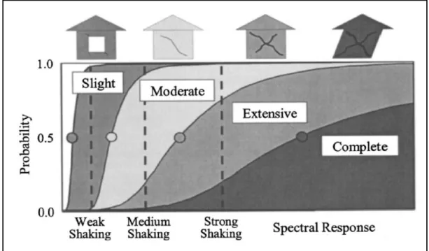
The HAZUS functions are the capacity curves and the fragility curves. As previously defined for the other methods, the capacity curves serve to determine the probability of damage of the structural elements and for both the drift-sensitive and acceleration-sensitive OFCs. Also, the fragility curves classify the damage into four physical damage states: slight, moderate, extensive and complete, as shown in Figure 1.10; more details about the damage functions can be found in Kircher et al. (1997) and in the software manual users guide (HAZUS, 1999).
Figure 1.10 Fragility curves for slight, moderate, extensive and complete damage (Source: Kircher et al. (2006))
The capacity curves are derived from pushover analysis for each building type and represent different lateral force resisting systems and building performance levels. These curves are defined by two control points, the yield capacity and the ultimate capacity, as shown in Figure
1.11. The yield capacity represents the elastic lateral strength and the ultimate capacity represents the maximum strength of the building when the structural system collapses as a full mechanism.
Figure 1.11 Example of a building capacity curve (Source: Kircher et al. (2006))
1.2.2 Qualitative assessment methods
1.2.2.1 Adapted rapid visual screening method (Tischer, 2012)
The adapted rapid visual screening method is a score assignment procedure proposed by Tischer (Tischer, 2012) to assess the seismic vulnerability of school buildings in Montréal. It is based on the capacity spectrum approach and adopts the same principles as the FEMA 154 method (FEMA454, 2006), with the introduction of the effect of structural irregularities. Therefore, the method considers six parameters: building height, type of lateral load resisting system, construction year, presence of structural irregularities, potential for pounding of
adjacent building(s), and local soil conditions (site classes are according to NBC). This screening method was applied to 101 school buildings designated as post-critical emergency shelters by the City of Montréal.
The seismic structural vulnerability of buildings is represented by an overall score S, which is equal to the summation of the basic structural hazard score (BSH) and various score modifiers related to each of the aforementioned parameters, as indicated in Equation (1.1)
S= BSH + Σ (score modifiers) (1.1)
For a given earthquake hazard, the BSH reflects the building performance based on the LLRS type according to FEMA 154. The score modifiers consider other features that make the building more or less vulnerable to seismic damage. The BSH is defined in Equation (1.2) as the negative logarithm of the probability of structural collapse under a specified extreme ground motion, the so-called maximum considered earthquake (MCE).
BSH= - log10 [P (collapse MCE)] (1.2)
The probability of collapse is estimated using the capacity spectrum method and fragility curves corresponding to various lateral load resisting systems (ATC, 2002). The expected seismic behaviour of a building is described by generic capacity curves. As mentioned before, the capacity curves give a relation between the lateral force and sway displacement in the structure and are defined by building type, height and quality of construction (ATC, 2002). The conditional probability of collapse is expressed in Equation (1.3).
P (collapse given MCE) = p (complete |dpi) x collapse rate (1.3)
Where p(complete |dpi) is the probability of being in complete damage state given a spectral displacement dpi, and the collapse rate is based on judgment and limited building collapse observations available for each type of LLRS identified in Table 1.1 and it is set to vary
between 0.03 and 0.15. This rate is based on failure modes where either local collapse of a wall or collapse of a single story, without significant ability of total structure collapse. The collapse rate will be greater than 15% if the building is expected to have a high probability of total collapse. Then, the BSH of each LLRS is evaluated based on the probability of collapse. The collapse rates of different building types for complete structural damage are taken from HAZUS-MH MR4 Technical Manual (NIBS, 2003) and given in Table 1.2. For more detailed description of the procedure of the determination of the collapse rates, the reader can refer to the HAZUS-MH MR4 Technical Manual.
Table 1.1 Types of Lateral Load Resisting Systems according to FEMA 154 (Adapted from ATC (2002))
Type FEMA154
Denomination Description
WLF W1 Wood light frame
WPB W2 Wood, post and beam
SMF S1 Steel Moment Resisting frame
SBF S2 Steel Braced Frame
SLF S3 Steel Light frame
SCW S4 Steel Frame with Concrete Shear walls
SIW S5 Steel Frame with infill masonry
shear wall
CMF C1 Concrete moment resisting frame
CSW C2 Concrete shear walls
CIW C3 Concrete frame with infill
masonry shear wall
PCW PC1 Precast Concrete walls
PCF PC2 Precast Concrete frame
RML RM1 walls with wood or metal deck Reinforced Masonry bearing floors
RMC RM2 Reinforced Masonry bearing
walls with concrete diaphragm
URM URM Unreinforced masonry bearing
Table 1.2 Collapse rates by model building type for complete structural damage
(Adapted from NIBS (2003))
Type OF LLRS Probability of collapse (complete damage state) WLF 0.03 WPB 0.03 SMF-L 0.08 SMF-M 0.05 SBF-L 0.08 SBF-M 0.05 SLF 0.03 SCW-L 0.08 SCW-M 0.05 SIW-L 0.08 SIW-M 0.05 CMF-L 0.13 CMF-M 0.10 CSW-L 0.13 CSW-M 0.10 CIW-L 0.15 CIW-M 0.13 PCW 0.15 PCF-L 0.15 PCF-M 0.13 RML-L 0.13 RML-M 0.10 RMC-L 0.13 RMC-M 0.10 URM-L 0.15 URM-M 0.15
L: Low rise; M: Medium rise
To calculate the score modifiers, SM, provisional scores are calculated using the same procedure as for the BSH, but the only difference is the input capacity and acceleration spectra. For example, to calculate the score modifier of a given LLRS for a specific soil type, the input acceleration will be according to the soil condition at the building site. Thus, the score modifier is obtained by subtracting the provisional score from the corresponding BSHs as shown in Equation (1.4). The proposed score modifiers are listed in Tables 1.3 and 1.4.
SM = BSH – provisional score (1.4)
Table 1.3 Basic score and score modifiers according to Tischer’s adapted screening method (Adapted from Tischer (2012))
LLRS B.M Year BSH Mid-Rise High Rise Irregularities
Vertical Plan W1 1970 5.2 0 0 -3.5 -0.5 W2 1970 4.8 0 0 -3 -0.5 S1 1970 3.6 0.4 1.4 -2 -0.5 S2 1970 3.6 0.4 1.4 -2 -0.5 S3 1970 3.8 0 0 0 -0.5 S4 1970 3.6 0.4 1.4 -2 -0.5 S5 1970 3.6 0.4 0.8 -2 -0.5 C1 1970 3 0.2 0.5 -2 -0.5 C2 1970 3.6 0.4 0.8 -2 -0.5 C3 1970 3.2 0.2 0.4 -2 -0.5 PC1 1970 3.2 0.4 0.6 -1.5 -0.5 PC2 1970 3.2 0 0 0 -0.5 RM1 1970 3.6 0.4 0 -2 -0.5 RM2 1970 3.4 0.4 0.4 -1.5 -0.5 URM 1970 3.4 -0.4 0 -1.5 -0.5
Table 1.4 Basic score and score modifiers according to Tischer’s adapted screening method
(Adapted from Tischer (2012))
LLRS Pre-Code Post B.M Soil C Soil D Soil E
W1 0 1.6 -0.2 -0.6 -1.2 W2 -0.2 1.6 -0.8 -1.2 -1.8 S1 -0.4 1.4 -0.6 -1 -1.6 S2 -0.4 1.4 -0.8 -1.2 -1.6 S3 -0.4 0 -0.6 -1 -1.6 S4 -0.4 1.2 -0.8 -1.2 -1.6 S5 -0.2 0 -0.8 -1.2 -1.6 C1 -1 1.2 -0.6 -1 -1.6 C2 -0.4 1.6 -0.8 -1.2 -1.6 C3 -1 0 -0.6 -1 -1.6 PC1 -0.4 0 -0.6 -1.2 -1.6 PC2 -0.2 1.8 -0.6 -1 -1.6 RM1 -0.4 2 -0.8 -1.2 -1.6 RM2 -0.4 1.8 -0.6 -1.2 -1.6 URM -0.4 0 -0.4 -0.8 -1.6
The overall score result of each building represents its structural vulnerability index that is further classified into four levels according to the ranking system of Table 1.5.
Table 1.5 Seismic vulnerability ranking system used in Oregon with FEMA 154 (Adapted from McConnell (2007))
Seismic vulnerability Probability of collapse under MCE Index value
Very high 100% ≤ 0.0
High 10% to 100% 0.1 - 1
Moderate 1% to 10% 1.1 – 2
Low Less than 1% ≥ 2
The score modifiers with their relative BSH presented in Tables 1.3 and 1.4 are those considered in the adapted screening method. For example, the building height has three categories: low rise (2-3 stories), mid-rise (4-6 stories) and high-rise (7 and more). In order to determine the provisional scores for the buildings, the spectral acceleration values used are the same as those for the Basic Structural Hazard score. The year of construction indicates the seismic provisions used in design; therefore, older buildings are expected to behave more poorly than more recent constructions. As per the FEMA method, two significant years are defined in Table 1.6: the Pre-code year, set as 1970 when the first probabilistic seismic zoning maps were introduced in the NBC, and the Benchmark year, 1990, when the ductility requirements were improved significantly, and inelastic behavior of the structures was taken into consideration in the NBC.
Table 1.6 Damage functions for seismic screening in Eastern Canada
Seismicity Post-Benchmark (1990) Pre-Code (1970)
Moderate & High Moderate Code Low Code Pre-Code
Low Low Code Pre-Code Pre-Code
The structural irregularities or weaknesses are classified as low or severe. Horizontal irregularities include re-entrant corners, asymmetric stairways, diaphragm discontinuity and asymmetric partition walls. Similarly, vertical irregularities include steps in elevation, the
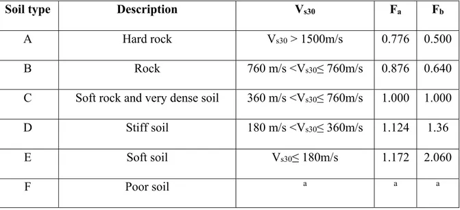
presence of soft story, sloping terrain and change in lateral load resisting system type. The soil type for a region may be determined from the available micro-zonation maps and geotechnical data. The value of the shear wave velocity can be estimated using the natural frequency and the depth of the sedimentary layer, and the average shear wave velocity up to a depth of 30 m, Vs30, can be used to determine the site class as per NBC. The provisional scores are calculated based on amplification of ground motion and the resultant increase in the spectral acceleration values. Table 1.7 lists the amplification factors for each soil type as well as the shear wave velocity for Montréal according to NBC.
Table 1.7 Ground motion amplification factors for Montréal, according to NBC 2015 (Adapted from NRC/IRC (2015))
Soil type Description Vs30 Fa Fb
A Hard rock Vs30 > 1500m/s 0.776 0.500
B Rock 760 m/s <Vs30≤ 760m/s 0.876 0.640
C Soft rock and very dense soil 360 m/s <Vs30≤ 760m/s 1.000 1.000 D Stiff soil 180 m/s <Vs30≤ 360m/s 1.124 1.36
E Soft soil Vs30≤ 180m/s 1.172 2.060
F Poor soil a a a
a: site-specific geotechnical investigation required
1.2.2.2 Manual for screening of buildings for seismic investigation, NRC 92 - Canada
Unlike the FEMA 154 (ATC, 2002) screening method, the NRC 92 method considers the vulnerability of operational and functional components. On the other hand, the FEMA 154 methodology is more accurate than NRC 92 in calculating the vulnerability scores because it is based on the capacity spectrum method.
The NRC 92 manual (NRC/IRC, 1992) is based on data collection by visual inspection of the building. This method determines a structural index dependant on five parameters: local seismicity, soil conditions, type of lateral load resisting system, presence of vertical and horizontal irregularities and building importance, in addition to a non-structural index that is function of the sources of non-structural hazards, the soil conditions and building importance. The sum of these two indices (structural and non-structural) provides a final score called the seismic priority index (SPI). According to NRC 92, the priority for seismic mitigation will be classified as a low if the SPI is less than 10 , as moderate if the SPI ranges from 10 to 20 , as high if the SPI ranges from 20 to 30 , and a potentially hazardous situation that requires immediate attention if the SPI score is larger than 30 (NRC/IRC, 1992).
1.2.2.3 CSA S832 - Seismic risk reduction of operational and functional components of buildings
In Canada, the standard CSA S832 “Seismic Risk Reduction of Operational and Functional Components of Buildings” (CSA, 2014) proposes a parametric method to evaluate the seismic risk associated with OFCs. The evaluation of the seismic risk involves the determination of the seismic vulnerability of the OFCs as well as the consequences of their failure. The seismic risk index of the component, R, is the product of the vulnerability index, V, and the consequence of failure index, C (Equation (1.5)).
R= V*C (1.5)
During an earthquake, the OFCs are subjected to inertial forces, deformation and impact due to their relative motion and possible interaction with other building components. The qualitative vulnerability index is related to the probability of failure of an OFC when the supporting building is subjected to seismic action. The vulnerability index is affected by a number of parameters that have been discussed in Section 1.2. According to Appendix A of CSA S832, the seismic vulnerability of the OFCs is function of their restraint, potential for
pounding and impact, their location and their flexibility. In accordance with the standard, in addition to the aforementioned OFC characteristics, the seismic vulnerability parameters include the effects of the magnitude of the ground motion and the flexibility of the structure. These parameters are weighted based on their relative importance and are used to calculate the vulnerability index, V (Clause 7.5.2.) according to Equation (1.6).
V= VG * VB* VE/10 (1.6)
VG is the ground motion characteristics index and is expressed in Equation (1.7) as the product of the spectral response acceleration value for a period of 0.2 s, Sa (0.2), and the acceleration-based site coefficient, Fa, that is defined in Article 4.1.8.4 of the NBC:
VG= Fa Sa (0.2)/1.25. (1.7)
VB is the building characteristics index, related to the flexibility of the structure expressed in terms of the type of the lateral load resisting system, the building fundamental natural period and the soil type, as per Table 1.8 (Clause A.4.4).The minimum and the maximum values of VB are 1.0 and 1.5, respectively.
Table 1.8 Building characteristics index according to CSA S832-14
Building fundamental period (s)
Lateral Load Resisting System (LLRS) 0 < T < 0.2s 0.2s < T < 0.5s 0.5s < T Number of stories
1-2 3-4 >5 Steel Moment Resisting Frame
1-2 3-5 >6 Reinforced Concrete Moment
Resisting Frame 1-2 3-7 >8 Concrete Shear Wall
1 2-4 >5 Braced Frame
VB VB VB Soil Type
1 1.1 1.2 Site Class A: Hard Rock
1 1.2 1.3 Site Class B: Rock
1.1 1.2 1.3 Site Class C: Very Dense Soil and soft rock
1.2 1.3 1.4 Site Class D: Stiff Soil 1.3 1.4 1.5 Site Class E: Soft Soil 1.5 1.5 1.5 Site Class F: Sandy Soil
VE is the OFC characteristic index obtained by the weighted sum of four rating scores according to the Equation (1.8):
VE = Σi=1,4 (RSi * WFi) (1.8)
RS1 represents the rating score for OFC restraint, RS2 is the rating score for OFC impact/pounding effects, RS3 is the rating score for OFC overturning and RS4 is the rating score for OFC flexibility. The weight factors WFi associated with each parameter are given in Table 1.9.
Table 1.9 Individual OFC parameters and weight factors according to CSA S832-14
Parameter Weight Factor
OFC Restraint 4
OFC Impact/Pounding 3
OFC Overturning 2
OFC Location and Flexibility 1
The OFC restraint represents the strength of connections between the OFC and the structural components. The OFC impact and pounding indicates the possibility of impact of the OFC on the other surrounding OFCs and structural components during ground shaking; therefore, an adequate gap should be provided between adjacent OFCs and between the OFCs and the structural components. The OFC vulnerability to overturning is represented by the height of the OFC centre of gravity above the floor level (h) relative to the dimension of its base (d). As per Clause A.4.2.3 of the standard, the maximum horizontal seismic force acting at the OFC centre of mass Vp is calculated according to Equation (1.9).
Vp = 1.2FaSa (0.2) WP (1.9)
Where WP is the weight of the OFC, Fa is the acceleration-based site coefficient and Sa (0.2) is the spectral response acceleration value at a period of 0.2s.
The OFC location and flexibility are represented by the floor level since the acceleration response typically increases with building height, which affects more the OFC located on the rooftop and at upper levels. The rating scores for the OFC vulnerability characteristic index VE are presented in Table 1.10 as provided in CSA S832.
Table 1.10 Rating scores for OFC characteristic index according to CSA S832-14
The consequence index, C, is determined from the anticipated consequences of the OFC failure. It is the sum of the rating scores related to life safety (LS), limited functionality (LF), full functionality (FF) and property protection (PP), based on the OFC seismic performance and the impact of its failure or malfunction. Table 1.11 presents the consequence rating scores based on the performance of the OFCs according to the CSA standard.
Vulnerability
Parameters Parameter Range Rating Score
Weight Factor OFC Restraint (RS1) Full Restraint 1 4 Partial Restraint 5 4 No Restraint 10 4 OFC Impact/Pounding (RS2) Gap Adequate 1 3 Gap Inadequate 10 3 OFC Overturning (RS3)
Fully Restrained against overturning or (h/d) ≤ 1/(1.2 Fo Sa (0.2)) (h/d) > 1/(1.2 Fo Sa (0.2)) 1 10 2 2
OFC Flexibility and Location in building
(RS4)
Stiff or Flexible OFC on or below ground floor
Stiff OFC above ground floor
Flexible OFC above ground floor 1 5 10 1 1 1
Table 1.11 Rating scores used for the determination of the consequence index of OFCs according to CSA S832-14
Consequence Parameters Parameter Range Rating Score (RS)
Life Safety (LS)
Threat to very few (N < 1) 1 Threat to few (1 < N < 10) 5 Threat to Many (N > 10) 10
Limited Functionality (LF)
OFC breakdown greater than
one week is tolerable 0 OFC breakdown up to 1 week is
tolerable 1
OFC in high importance category building and that is not
required to be fully functional
3
OFC in post-disaster facility and that is not required to be fully
functional
5
Full Functionality (FF)
Not Applicable 0
OFC required to be fully
functional 10
Property Protection (PP)
Score may vary from 0 to 10 as determined by the owner /
Operator
0-10
As mentioned in Appendix C (Clause C.1) of the CSA standard, the seismic risk is calculated for prioritized mitigation so that for an OFC located in a normal importance category building with a seismic risk index (R) less than or equal to 16, mitigation is not required due to limited benefits of risk reduction. The priority for mitigation should be established after risk assessment based on the determined risk index (R) according to Table 1.12.
Table 1.12 Suggested mitigation priority thresholds according to CSA S832-14
Risk Index Seismic Risk Level Mitigation Priority
R < 16 Negligible Not required
16 < R < 32 Low Low
32 < R < 64 Moderate Medium
64 < R < 128 High High
R > 128 Very high Very high
1.3 Previous studies on post-earthquake functionality of buildings
The post-earthquake functionality of a building is largely dependent on the survival of its non-structural components as well as the good performance the non-structural resisting system. For schools designated as post-disaster shelters, loss of functionality could be critical.
In order to assess the post-disaster functionality of residential buildings, a stochastic study was done at the University of Oklahoma, USA (Lin & Wang, 2017b), introducing a building portfolio recovery model (BPRM) to estimate the stochastic recovery of buildings following a hazardous event (Lin & Wang, 2017b). The BPRM contains five functionality states such as the restricted entry (RE), restricted use (RU), re-occupancy (RO), baseline functionality (BF), and full functionality (FF). These states are defined as the performance index of a building, which is modeled using discrete-state representing a portfolio-level recovery by computing the building level restoration in temporal and spatial dimensions, using continuous-time Markov Chains (CTMC). Figure 1.12 represents this analysis procedure.
Figure 1.12 Analysis procedure in the building portfolio recovery model (BPRM) (Source: Lin & Wang (2017b))
The first step in the building portfolio recovery method is the pre-recovery (initial) functionality status immediately at the time of occurrence of the earthquake (t0). This step involves the assessment of the initial functionality state before the beginning of any recovery activity. That type of assessment is usually done by engineers according to the ATC-20 (Oaks, 1990) and the functionality losses need to be estimated according to a probabilistic approach as shown in Figure 1.13.
Figure 1.13 Flowchart of the probabilistic approach of pre-recovery damage and functionality loss assessment
As shown in Figure 1.13, the probabilistic approach proceeds by estimating the damage of the structural components (𝐷𝑆 and of both the drift-sensitive (𝐷𝑆 and the acceleration-sensitive (𝐷𝑆 ) non-structural components for a given earthquake scenario. Mapping or overlaying the structural component damage state and the non-structural component damage states with the availability of utility service of the building, Un, will result in the building-level functionality state probabilities and the portfolio-level functionality recovery index, PRI, as a function of t0. The second step following the pre-recovery functionality assessment is the building portfolio functionality recovery prediction for a period of time larger than t0 (t > t0). Based on the pre-recovery step, a recovery analysis is conducted to estimate the building-level restoration functions (BRF) and portfolio-level recovery trajectory, PRIj(t), and the recovery time PRTFF,95% which is the time needed to restore 95% of the building to full functionality (Lin & Wang, 2017a). The BPRM can be summarized in Figure 1.14.
Figure 1.14 Building damage and utility availability to building functionality states (Source: Lin & Wang (2017a))
1.4 Previous studies on the effects of soil-structure resonance
The soil-structure resonance phenomenon is an important aspect of the dynamic behavior of a structure subjected to a ground motion. Resonance amplifies the seismic response of the building and leads to potential structural and non-structural damage, especially if internal structural damping is low. It may also lead to soil liquefaction in vulnerable sites (Soil Class E). Resonance will occur when the site period and the fundamental period of the building are close to each other (Bolander et al., 2001). Figure 1.15 shows a schematic graph of the amplification of building accelerations due to soil-structure resonance.
Figure 1.15 Effect of resonance on the seismic response of buildings (Source: FEMA454 (2006))
As larger lateral inertia forces are induced at resonance, soil-structure resonance can strongly increase the building deformations (Kvasnicka et al., 2011) and damage to drift-sensitive OFCs.
Mucciarelli et al. (2004) have analyzed the effect of soil-building resonance and the elongation of the fundamental period of the structure due to stiffness reduction induced by structural damage after the successive October 31 Mw 5.4 and November 1, 2002 Mw 5.3 earthquakes
that occurred at the border between Molise and Puglia in Southern Italy. To test if the soil-building resonance had increased the structural damage, ambient vibration data were recorded inside the most damaged building after the first earthquake, then during and after the second one. The recorded data were analyzed to estimate the fundamental frequency of the building and its shift (period elongation) due to damage. The analysis was done using many techniques such as the Short-Time Fourier Transform (STFT), Wavelet Transform (WT), Horizontal-to-Vertical Spectral Ratio (HVSR) and the Horizontal-to-Horizontal-to-Vertical Moving Window Ratio (HVMWR). To estimate the fundamental frequency of the soil supporting the building, three different techniques were applied such as noise HVSR, Strong motion HVSR of seven aftershocks, and 1-D modeling (soil column) based on a velocity profile derived from noise analysis of surface waves (NASW). The different measurements led to the conclusion that the fundamental frequency of the most damaged building is in the same range as the fundamental frequency of the underlying soft sediments before the damage, thus proving that soil-building resonance effects had occurred during the earthquakes.
During the assessment of the seismic vulnerability of school buildings in Tehran City, Iran, Panahi et al. (2014) also considered the seismic resonance coefficient as a main factor affecting the structural vulnerability. Therefore, the resonance coefficient was simply taken as the ratio of the fundamental period of the structure to that of the soil underneath.
Tezcan et al. (2012) concluded that the main reason for the collapse of the Paint Workshop of the Tofas-Fiat automobile factory building in Bursa during the 1970 Mw 7.2 Turkish earthquake was due to soil-structure resonance effects.
As can be concluded from previous studies and observations in past earthquakes, coincidence of the natural period of the structure and that of the supporting soil will lead to significant response amplification that results in increased damage and even collapse. Therefore, during this study it is deemed very important to check the potential for soil-structure resonance.
1.5 Analytical Hierarchy Process (AHP)
The Analytical Hierarchy Process introduced by Saaty (1977) can be used in a wide variety of decision-making processes such as in business, insurance, industry and education. AHP is one of the most commonly used multi-criteria decision-making methods, and is based on the calculation of the relative importance of each parameter affecting the main goal of the study via a pairwise comparison. Then, it transforms the comparison into numerical values that are further processed in a mathematical matrix format. Note that the compared parameters are statically independent, which means that while comparing two parameters affecting the structural vulnerability the other parameters won’t affect this comparison. The relative importance of the parameters is identified by assigning a weight factor to each of them based on the scale of preference between each pair of parameters as shown in Table 1.13.