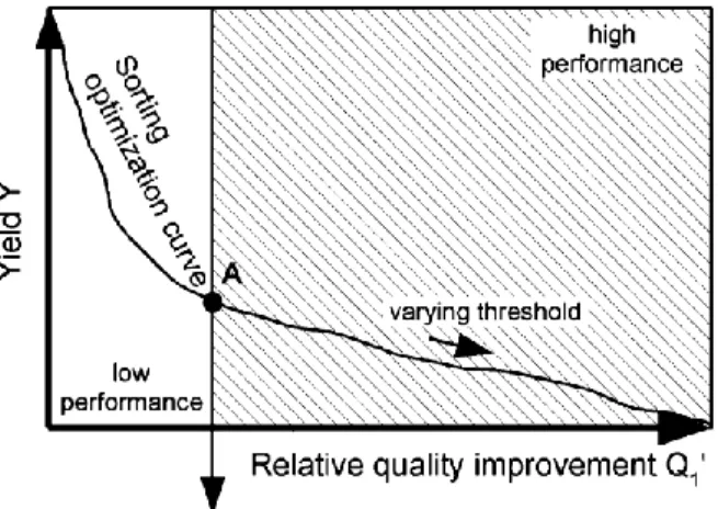
A sorting optimization curve with quality and yield requirements
D. Ooms, R. Palm, V. Leemans, M.-F. Destain
University of Liège, Gembloux Agro-Bio Tech, 2 Passage des Déportés, B-5030 Gembloux, Belgium
ABSTRACT
Binary classifiers used for sorting can be compared and optimized using receiver-operating characteristic (ROC) curves which describe the trade-off between the false positive rate and true positive rate of the classifiers. This approach is well suited for the diagnosis of human diseases where individual costs of misclassification are of great concern. While it can be applied to the sorting of merchandise or other materials, the variables described by the ROC curve and its existing alternatives are less relevant for that range of applications and another approach is needed. In this paper, quality and yield factors are introduced into a sorting optimization curve (SOC) for the choice of the operating point of the classifier, associated with the prediction of output quantity and quality. Given examples are the sorting of seeds and apples with specific requirements. In both cases the operating point of the classifier is easily chosen on the SOC, while the output characteristics of the sorted product are accurately predicted.
Keywords : Binary classification ; Classifier optimization ; ROC ; SOC ; Sorting ; Threshold
1. Introduction
Among the binary classifiers used for sorting, discretized probabilistic classifiers are very common. In these classifiers, each object data Dx is characterized by a set of features whose values are stored in the vector x. Using
the data of a training set and a defined rule that depends on the sub-type of classifier (discriminant analysis, non-parametric Bayes classifier, backpropagation neural network, etc.), the classifier outputs a value y. Low values of
y indicate a high probability that the objects belong to the outlier class ω0 (foreign materials and other
undesirable objects), and high values of y indicate a high probability that the object belongs to the target class ωt.
A threshold t is introduced to obtain a discrete classifier usable for sorting:
where "Accept" is the positive fraction and "Reject" the negative fraction after sorting.
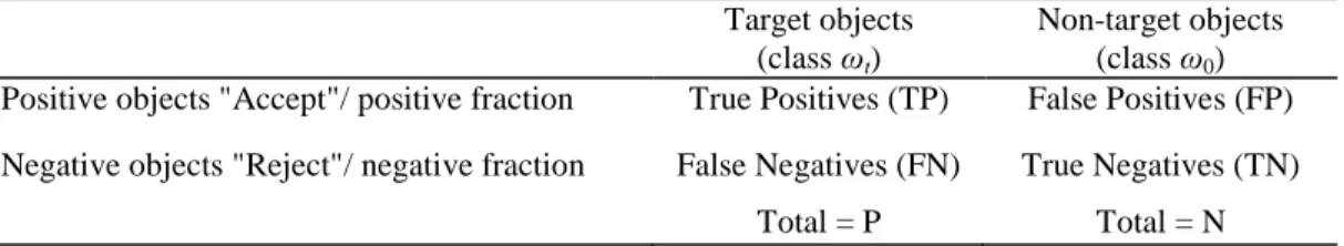
The result may be listed into a confusion matrix (Table 1). Notations P, N, TP, FP, TN and FN are from Fawcett (2006a). ωt and ω0 are from Landgrebe et al. (2006). The "Hypothesized classes" Y and N from Fawcett (2006a)
were not used and replaced by "Accept" and "Reject" to avoid confusion with other variables.
It is most often possible to modify the output TP, FP, FN, TN of the sorting process by varying the threshold t. To perform the classifier optimization, a performance criterion is needed, which depends on t. The performance of a classifier may be assessed in several ways. Some of the most commonly used are (with example): accuracy (Lai et al., 2009), Cohen's Kappa coefficient (Edlund and Warensjö, 2005) and the receiver-operating
characteristic (ROC; Bukovec et al., 2007). Accuracy is:
It does not take into account the occurrence of correct or incorrect classification happening by chance. Accuracy does take into account neither the misclassification costs nor the advantage to increase the quality of the output at the cost of material losses. The Cohen's Kappa coefficient (Cohen, 1960) is a more robust estimator of the classifier performance than accuracy, since it takes into account the agreement occurring by chance. The ROC curve (as described in Bradley, 1997; Webb, 2002; Fawcett, 2006a) is a representation of the trade-off between the two types of sorting errors as a function of t. These errors are tied to the ratios FPr and TPr and refer to the notions of specificity and sensitivity of a classifier:
TPr: true positive rate = TP/P; FPr: false positive rate = FP/N. Specificity and Sensitivity are:
Maximizing both sensitivity and specificity at the same time is not possible, since they vary in opposite direction when the decision threshold t varies. These two parameters are usually represented into a receiver-operating characteristic (ROC) curve. A ROC curve is a graphical plot of the true positive (TPr) vs. false positive rate (FPr) (Fig. 1). On such a graph, sensitivity is expressed as a function of (1-specificity) for a given classifier and a given population, but an analytic expression only exists under simple assumptions, e.g. Gaussian conditionals. In most cases, the ROC curve is built by testing the classifier on the basis of samples (e.g. Faustini et al., 2007). ROC curves are often used for medical diagnosis applications (e.g. lung abnormality detection: Tagashira et al., 2008).
ROC graphs may be used for two main purposes:
- the comparison of different classifiers used for the same task (e.g. Vergara et al., 2008);
- the optimization of the value of threshold t, or in other words the choice of an operating point for a given classifier.
Fig. 1. A ROC curve. Hatched: zone satisfying the specificity criterion. A: Operating point with best sensitivity satisfying the specificity criterion, following the Neyman-Pearson method. Inverted classifier: Inverting the output classes gives a curve located to the other side of the dashed line.
Table 1 Composition of the sorted fractions.
Target objects (class ωt)
Non-target objects (class ω0)
Positive objects "Accept"/ positive fraction True Positives (TP) False Positives (FP) Negative objects "Reject"/ negative fraction False Negatives (FN) True Negatives (TN)
Total = P Total = N
1.1. Comparison of classifiers
The area under ROC curves (AUC) is used as an indicator of the overall classifier performance (Bradley, 1997). It is also the integral between 0 and 1 of the function TPr = f(FPr) if such a function exists. AUC is used to compare classifiers. Each classifier is built using the same training set. A unique testing set, separate from the training set, is then used for the estimation of the operating points of the ROC curves corresponding to each classifier. The uncertainty on the estimated AUC is discussed in (Yousef et al., 2005).
1.2. Choice of the optimal operating point
The operating point is chosen in order to maximize both sensitivity and specificity with the aim to approach the upper-left corner of the graph ('perfect result'). There is no general definition of the optimal operating point. Sometimes, some requirements must be met for sensitivity, specificity, or both. The Neyman-Pearson rule (Webb, 2002) consists in plotting these requirements into the graph and finding an operating point belonging to the ROC curve, corresponding to a particular value of t, which maximizes specificity for a particular value of sensitivity, or inversely. This particular value is a boundary to the "meet requirements" zone (hatched, Fig. 1). The implication of error costs is introduced in (Chow, 1957). A cost-based estimation of the optimal operating point on ROC curves is given in (Tortorella, 2000; Santos-Pereira and Pires, 2005). The analytical solution to the optimization of a sorting process (distributed hypothesis-testing problem) using Neyman-Pearson strategy is given in (Elayadi et al., 1996), However, this solution is specific to a particular classifier.
1.3. Alternatives to the ROC curve
Some alternatives to the ROC curve exist. Fawcett (2006b) proposed a modified curve called ROCIV graph that may accommodate costs of misclassification. These costs must be defined for each application. Other
alternatives to ROC curves include the skill plot (Briggs and Zaretzki, 2008). The skill is an estimation of the value of a particular test compared to a naïve test. It is still based on the individual misclassifkation costs. These alternatives are focused on the individual misclassifkation costs resulting from wrong diagnosis in medical applications. They are not adapted to production applications where objects are merchandise or food materials because their sorting requires other criteria such as output purity and value. Feller et al. (1994) proposed a method of describing sorting efficiency of machines independently of feed composition P/N. However, it is not suitable for choosing an optimal operating point (sorting parameters).
1.4. Objectives
This paper focuses on the sorting of objects whose quality is quantifiable and dependent on the amount of objects from ωt and ω0 into the output. The quality improvement of objects in industry and agroindustry involves
two requirements:
- the rejection of foreign materials;
- the improvement of pure product by elimination of damaged, broken, discoloured, or other unwanted objects, and the sorting of different categories of product.
The first task is largely implemented using simple sensors and direct rejection of unwanted objects. An example is the automatic identification of contaminants in recycled glass materials (Kattentidt et al., 2003). The second application ranges from the simplest (sorting by size using sieving methods) to the most challenging problems, such as the detection of recent bruises on apples (Kleynen et al., 2005). Other examples of possible applications include the sorting of corn kernels (Liao et al., 1993), rice kernels (Wan, 2002), wheat kernels (Luo et al., 1999), soybeans (Casady et al., 1992; Wang et al., 2002) and ore (Cutmore et al., 1998). Recently, techniques such as image processing are used to extract more relevant information from images of the objects. While most
applications found in the literature are associated with a high classification performance, even an inaccurate classifier may bring valuable results with the appropriate tools for choosing the classifier parameters, in particular the decision threshold. This will be demonstrated with the examples.
The objective is to provide a tool for the set-up of a sorting process including quality and yield constraints which are often required in a production environment. Quality can be a legal requirement, a criterion to a market standard, or a requirement from the producer to meet his particular needs. On the other hand, material losses must be avoided and yield is thus also a major issue. Furthermore, the proposed tool should be applicable to a large number of classifiers commonly used for that task. Finally, the new tool should express the results into a form that allows an easy choice of an optimal operating point (i.e. value of t) for the classifier.
The paper is organized into the following sections. The introduction is presented in the first (present) section. Specific performance criteria for a classifier are introduced and plotted onto a sorting optimization curve and the determination of optimal classifier settings are commented in the second section (method). Two examples of applications are presented in the third section (results): the sorting of seeds on the basis of imaged chlorophyll fluorescence and the sorting of apples based on defect recognition.
2. A sorting optimization curve adapted to quality and yield requirements
2.1. The variables commonly used in binary classification and sorting
The proposed sorting optimization curve uses the same approach as the classical ROC: i.e. the quality and yield are computed from confusion matrix entries. The difference is in the specification and interpretation of the "costs" which are transformed into variables representing other concepts. Therefore, existing algorithms may be applied to the SOC.
The objects are sorted into two fractions: "Accept" and "Reject". Some of the terms defined above need to be adapted for the sorting application:
positive: sorted into the "Accept" output fraction or positive fraction; negative: sorted into the "Reject" output fraction or negative fraction; true: correctly sorted;
false: erroneously sorted.
ωt: target class, or wanted objects, corresponding to TP and FN;
ω0: non-target class, or unwanted objects, corresponding to TN and FP;
TP, TN, FP, FN, TPr, FPr, specificity, selectivity and accuracy remain unchanged. The following variables are specific to the sorting of objects:
Pt0: proportion of target objects in the whole population;
Pt1: proportion of target objects in "Accept" (= purity or precision, Landgrebe et al., 2004);
Q0: quality of the whole population of objects before sorting;
Q1: quality of the population of objects in "Accept";
Y: sorting yield;
Pt, Q and Y will be expressed in Section 2.2 in function of the other parameters.
2.2. The variables represented by the sorting optimization curve 2.2.1. Quality
A set of objects is sorted to improve its quality and value. The term quality has to be understood as defined above (legal requirement, criterion to a market standard, or requirement from the producer). The term "quality" is applied to the set of objects, not to the classifier. We wish to compare the quality of the initial objects to that of the objects contained in the positive fraction, since objects from the negative fraction are not intended to be used. The common characteristic of a set of objects, whatever their nature, is the proportion of target objects in the set. Before sorting, the proportion of target objects is:
proportion of target objects in the lot before sorting. It is expressed anticipatively in function of the final amounts.
After sorting, the proportion of target objects in the positive fraction is:
Pt1 is the proportion of target objects into the positive fraction after sorting, corresponding to the positive
predicted value (PPV; Bradley, 1997; Fawcett, 2006a), purity (Landgrebe et al., 2004) or precision (Landgrebe et al., 2004; Fawcett, 2006a).
This paper focuses on the passage from the original objects to the improved positive fraction. While the negative fraction is not always worthless (as for the example of apples below), the negative fraction is by default
considered as a loss. However, in the same example the residual value of the negative fraction could be interpreted without difficulty.
Let us define a positive function f representing the relationship between the quality of the product and the proportion of the target objects:
The above definition applies to the quality before sorting: Q0 = f(Pt0), or after sorting for the positive fraction: Q1
= f(Pt1) using the same function ƒ. The function ƒ may not be linear, and a high proportion of target objects may
signify a greatly increased quality and value. In other cases, Q may be simply proportional or equal to Pt. Q may refer to unit price for commercially sold objects such as apples, or to a much more qualitative notion for sorting applications within the context of research, such as the sorting of micro-scale object particles (Hayashi et al., 2008). As the definition of quality varies greatly with the application, it is important to leave some freedom for the choice of ƒ. The only constraint is normalization such as:
Below are given some examples of functions ƒ.
2.2.1.1. Example 1 : Seed sorting. Target objects are seeds that germinate if placed in appropriate conditions.
The quality is proportional to the amount of germinating seeds in the seed lot and Q = Pt (solid line, Fig. 2). The output quality is therefore equal to the precision. The sorting operation is not the final stage of the production and the operator does not choose to introduce commercial value into the equation of Q.
2.2.1.2. Example 2: Sorting of apples. Target objects are apples sufficiently healthy to be accepted as "Category
I" (OCDE standard), while non-target objects are apples with defects not acceptable in this category. A tolerance of 10% is applied to the amount of unhealthy fruits after sorting. We make the hypothesis that a batch of apples not accepted in Cat. I (with less than 90% of healthy fruits) can be sold at half the price. The operator chooses to define the quality as proportional to the expected unit price of the positive fraction. The limit of 90% is not strict, since the apples will be quickly examined by an expert at the market place. A sigmoid is used to represent this uncertainty (Fig. 2, dashed line):
Possibly, a requirement QRis set on the output quality Q1 of the positive fraction:
with QR being a value set by the operator.
It has interesting properties. Significant negative values represent a classifier where classes are inverted. A value of 0 corresponds to a completely inefficient classifier and a value of 1 corresponds to a perfect output quality. The notations for the quality requirement QRor QR' correspond to the use of Q1 or Q1' respectively.
Fig. 2. Two examples of functions Q = f(Pt): seeds (solid) and apples (dashed).
2.2.2. Quantity or yield
On the other hand, the operator wants to maximize yield, the yield being usually the amount of output product in the "Accept" class compared to the total input. It corresponds to the amount of objects in the positive fraction of a sorting operation (Landgrebe et al., 2004):
Alternatively, the following expression could be used:
With Y, no distinction is made between false and true positive when selling the product. Both count in the amount sold. Y would be used in the case where false positive are not considered as product, but as additional material affecting the quality and not intended to be sold.
The producer may also have a requirement about yield YR associated with the condition:
2.3. Building of the sorting optimization curve
Prior to the building of the SOC, the classifier must be chosen, built and trained. The method for building a sorting optimization curve (Fig. 3) is:
- determine the usable values of the threshold t for the classifier;
- compute TP, TN, FP and FN for each value of t using data unseen when training the classifier; - compute Q1' (or Q1 and Y (or Y') from TP, TN, FP and FN for each value of t;
- report these values on a 2D graph and annotate the corresponding values of t;
- draw the requirements on quality (QRor QR') and/or yield YR as straight lines on the graph.
The operating points of the sorting optimization curve are built from at least one labeled data set having a particular value of Q0. The curve is sensitive to Q0 and therefore, sensitive to Pt0 and class skew. A computer
may be used to simulate the variation of Q0 by varying the priors of the classifier and rebuild the new
optimization curve automatically. If the shape of the feature distributions are not dependent on the priors, the priors may be varied by randomly suppressing the data from either ωt or ω0. Otherwise, additional independent
data sets with different priors should be used to rebuild the SOC. The problem is similar to that of the use of the ROC in the case of varying class distributions, discussed by Webb and Ting (2005).
The use of the bootstrap technique (Palm, 2002) allows the resampling of the two data sets used for model training and for the estimation of the operating points of the SOC. The resulting SOC is therefore an average of several model training and testing operations. This was used in the first example (Section 3.2).
Fig. 3. The sorting optimization curve with quality requirement, but no yield requirement. Hatched: Zone satisfying the quality criterion. A: operating point with best yield satisfying the quality criterion, following the Neyman-Pearson method.
2.4. The optimum operating point on the sorting optimization curve
In most cases, the optimum operating point must be located within the "meet requirements" zone. A compromise is needed if the requirement cannot be met but is not strict. For the maximization of both yield and quality, a criterion is needed.
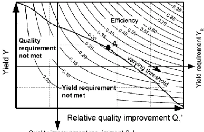
An easy way to find the best operating point is to define the sorting efficiency as following:
This leads to curves that can be superimposed to a surface chart (Fig. 4). This parameter reflects the part of the work done by the sorting process.
The optimum efficiency is then determined by finding the highest point of the optimization curve on the surface, within the requirements by either the operator or a computer (Point A, Fig. 4).
Fig. 4. Sorting optimization curve with quality and yield requirements. A: Operating point with maximum efficiency satisfying the requirements.
3. Examples
3.1. Introduction to the examples
These examples are intended to illustrate the implementation and usefulness of the SOC. Real data were collected or recovered from a previous study and used to build SOCs. The context in which the SOC would be used is also real, but at a smaller scale regarding the amount of available data (in the second example, the efficiency of the classifier is underestimated in comparison with the original study). The possible exploitation of the results is extrapolated.
3.2. The sorting of seeds
In this example a classifier is optimized with the aim of sorting chicory seeds, provided by Chicoline®, a division of Warcoing S.A. (Warcoing, Belgium), using a feature extracted from chlorophyll fluorescence imaging. The two output classes correspond to:
- seeds which germinate and present a normal embryo if placed in standard conditions (I.S.T.A., 2005) (target objects), and
- other seeds (non-target objects).
As non-germinated seeds do not produce any plants in the field, the quality function ƒ was defined in Section 2.2.1 and is simply equal to Q = ƒ(Pt) = Pt. A minimum quality requirement QRis fixed to 93% (Pt1 must be
≥0.93). However, QRis only the final requirement of the sorting process and is not strict, since other sorting
machines are available to improve Pt and quality. The initial quality Q0 is 0.854 ± 0.018 (α = 0.05; α refers to
confidence level).
The classifier used is based on the Bayes theorem with non-parametric estimation (kernel method) of probability densities, as described in (Webb, 2002). At the final stage of classification, threshold t is used on P(ωt|x) to
classify the object i:
and
with P(ωt|x) being the probability for an object characterized by feature vector x to belong to target class.
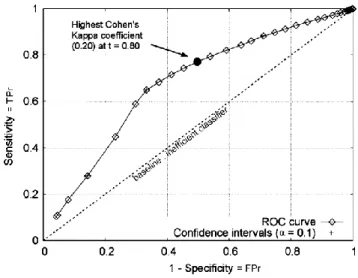
Fawcett, 2006a) of 200 estimations each based on bootstrap samples (Palm, 2002) taken from 850 individual seeds. For each sampling, approximately two thirds of the data were used for the estimation of the above probability densities and the remaining third for the estimation of the classifier performance. The choice of an optimal operating point is difficult on the basis of this graph alone. The point corresponding to the highest Cohen's Kappa coefficient is t = 0.80, but there is no information about the output quality. The confidence intervals of the mean estimation are shown in the figure (small crosses) at three different thresholds (0.7, 0.88 and 0.94).
Fig. 5. The ROC curve of the classifier, α: Confidence level of the confidence intervals.
Fig. 6. Sorting optimization curve of the classifier using the same base data as for Fig. 5. t: threshold; E: efficiency= Q1'Y. Dotted line: upper confidence limit on the quality requirement, QR'.
The sorting optimization curve was plotted by varying t and estimating the resulting Q1' and Y after classifying
validation data not used for training (Fig. 6). The quality requirement QR= 0.93 corresponds to QR' = 0.52 with
the confidence interval of QR' deducted from the confidence interval on the initial quality. The confidence
The upper confidence interval limit, QRA'. is used as the requirement on quality improvement.
QR' may have a different confidence level (here α = 0.05) than those of the individual points of the SOC (α =
0.1). The use of confidence intervals is not required and their confidence level may be chosen freely. However, they must be taken into account when reading and interpreting the curve.
The elements of Fig. 6 are described below:
(1) The sorting optimization curve (SOC, diamonds) is obtained according to the method described in Section 2.3. The Y and Q1' values are means obtained from 200 bootstrap samples (threshold averaging).
(2) The confidence intervals of the mean estimation of the SOC points (α = 0.1) are drawn for t = 0.94, t = 0.88 and t = 0.7 (crosses). The result of a particular sorting operation is expected to be into these intervals for a high number of sorted objects (N + P → ∞), as expected for seeds.
(3) The upper limit of the confidence interval on QR' is plotted as a dotted line.
(4) The efficiency, E, is mapped as a surface chart.
The operating point which satisfies the quality criterion (QR' ≥ 0.57) with the highest yield is around t = 0.97. If
the quality requirement is not strict, the operating point at t = 0.88 is more interesting with Q1' ≥ 0.455
(probability = 95%) and a higher yield (Y ≥ 0.6, probability = 95%). It also corresponds to the maximum efficiency E = 0.27. The operating point at t = 0.88 is also the furthest from the baseline of the ROC curve (dashed in Fig. 5) but the fact that it is mere coincidence or not has still to be debated.
Consequently, the use of this combination feature/classifier may lead to a quality improvement of the product from Q0 = 0.85 to Q1 = 0.895, corresponding to Q1' = 0.3 with limited losses (yield = 0.6) when using t = 0.88.
Using a higher threshold (t = 0.97), the quality requirement can be met (from Q0 = 0.85 to Q1 = 0.935,
corresponding to Q1' = 0.58) at the cost of high losses (yield value around 0.15).
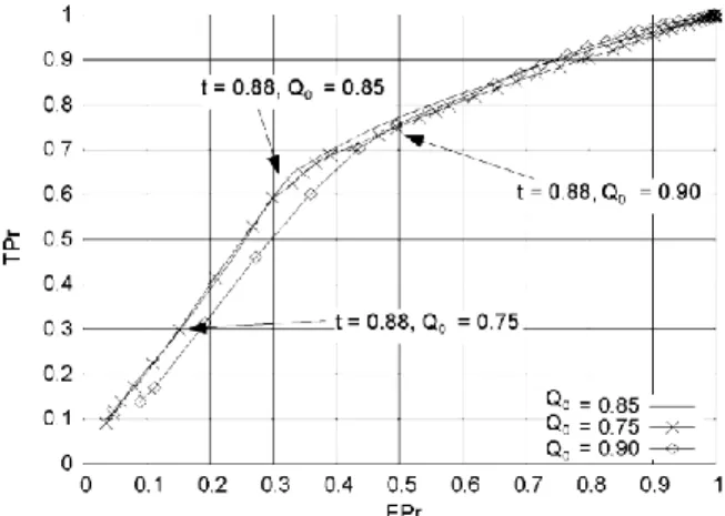
Finally, the sensitivity of the ROC curve (Fig. 7) and sorting optimization curve (Fig. 8) to Q0 was estimated
using three different values of Q0 (0.75, 0.85 and 0.9). The first and third values were simulated by randomly
suppressing the data corresponding to viable or non-viable seeds. The contour of the ROC curve is insensitive to class skew (Fawcett, 2006a), and therefore to Q0∙ The contour variation shown in Fig. 7 is only due to random
sampling effects. This property is not shared by the sorting optimization curve due to the dependence of Q on Pt. Moreover, the position of the point corresponding to a particular threshold is highly variable for all curves. The sorting optimization curve must be rebuilt for the current value of Q0 if it is used to choose the operating point.
Fig. 7. Estimation of ROC curve using three different values of Q0 Contour variations between curves are due to
Fig. 8. Estimation of the sorting optimization curve for three different values of Q0.
Fig. 9. A sorting optimization curve designed for the sorting of apples.
3.3. The sorting of apples
The automated sorting of apples is not widely implemented and still requires human intervention. However, there is an increased interest for the automation of that task as shown in the works of Leemans and Destain (2004), Throop et al. (2005), Kleynen et al. (2005), Xing and De Baerdemaeker (2007) and Kavdir and Guyer (2008) among others. On the basis of the quality function given in Section 2.2.1 for apples, a sorting
optimization curve has been built (Fig. 9). Apples from the Jonagold variety were used to train and test the classifier. The classifier used is based on the Bayes theorem with parametric estimation of probability densities (discriminant analysis). The whole methodology is described by Kleynen et al. (2005). Some data from the authors were used to build the SOC The available amount of data not previously used for model training (73) was sufficient to build a SOC, but not as accurately as suggested below. The digits of precision were left for the purpose of legibility and this does not affect the methodology. The estimation of SOC errors in the case of small sampling may be the topic of a further work.
We make the hypothesis that a producer has a requirement on yield since he must deliver at least 2 × 10³ kg of Class I apples from an initial quantity of 20 × 103 kg of unsorted apples. The yield requirement is thus 0.1. The initial proportion of healthy apples is Pt0 = 0.494. The producer does not want to take the risk to deceive his
client and set a quality requirement QR= 0.95, corresponding to a probability of 90% for the lot to be accepted as
Class I. According to the SOC (Fig. 9), no operating point can satisfy the two requirements simultaneously. However, the automated sorting is not useless. The operating point satisfying the quality requirement with maximum yield corresponds to t = 0.894 with Y = 0.065. The amount of apples that may be provided by automatic sorting is then 0.065 × 20 × 103 kg = 1.3 × 10³ kg.
After sorting, 18.7 × 10³ kg of apples remain, corresponding to the negative fraction with a proportion of healthy apples of 46%. The remaining 700 kg of "Cat I" apples must be provided by manual sorting. We make the hypothesis that the apples issued from the manual sorting cannot be mixed homogenously with those issued from the automated sorting and that the better quality output of manual sorting cannot be exploited to decrease the quality requirement of the automated sorting.
Considering the same quality requirements for the manual sorting (Ptm1 = Pt1 = 0.92, the operator voluntarily
selects 8 unhealthy apples for every 92 healthy apples), the amount of apples that must be sorted manually to provide the remaining 700 kg of "Cat I" apples is:
If the people involved with manual sorting select only healthy fruits, Ptm1 = 1 and the amount becomes:
Without the help of automated sorting, the amounts of apples to be manually sorted are 3.72 x 10³ or 4.05 x 10³ kg, respectively, to Ptm1 = 0.92 and Ptm1 = 1. This example demonstrates that even a poorly efficient classifier
may be exploited for automated sorting with the help of the SOC. 4. Conclusion
The sorting of objects, whose value depends on the amount of non-target objects into the output, is better handled using quality improvement and yield factors into a sorting optimization curve (SOC) instead of the True Positive and False Positive rates as for the building of receiver-operating characteristic (ROC) curves. The method allows an easy interpretation of the curve from a practical point of view and expresses the results into a form that makes it possible to choose an optimal operating point for the classifier involved in the sorting process. This operating point is associated with the prediction of output quantity and quality. The sorting optimization curve is sensitive to class skew. It is therefore recommended to periodically augment and update the SOC database to include all the most common cases encountered in practice. The method is general and can be applied to fruits, seeds, minerals, processed food and other objects. The exact estimation of errors and confidence intervals may be the next step into the study of the SOC.
Acknowledgements
This study was funded by the D.G.T.R.E (General Directorate of Technology, Research and Energy) of the Walloon Region, Belgium, following a European project "First-Europe, Objective 1". All calculations were made using GNU Octave (http://www.octave.org).
References
Bradley, A.P., 1997. The use of the area under the ROC curve in the evaluation of machine learning algorithms. Pattern Recognition 30 (7), 1145-1159.
Briggs, W.M., Zaretzki, R., 2008. The skill plot: A graphical technique for evaluating continuous diagnostic tests. Biometrics 63, 250-261. Bukovec, M., Špiclin, Z., Pernuš, F., Likar, B., 2007. Automated visual inspection of imprinted pharmaceutical tablets. Measur. Sci. Technol. 18, 2921-2930.
Casady, W.W., Paulsen, M.R, Reid, J.F., Sinclair, J.B., 1992. A trainable algorithm for inspection of soybean seed quality. Trans. ASAE 35 (6), 2027-2033.
Cohen, J., 1960. A coefficient of agreement for nominal scales. Educ. Psychol. Measur. 20, 37-46.
Cutmore, N.G., Liu, Y., Middleton, A.G., 1998. On-line ore characterisation and sorting. Miner. Eng. 11 (9), 843-847. Edlund, J., Warensjö, M., 2005. Repeatability in automatic sorting of curved Norway spruce saw logs. Silva Fenn. 39, 265-275. Elayadi, M.H., Mamdouh, A, Basiony, A.E., 1996. An algorithm for global optimization of distributed multiple-sensor detection systems using Neyman- Pearson strategy. Signal Process. 51, 137-145.
Faustini, M., Battochio, M., Vigo, D., Prandi, A., Veronesi, M., Comin, A., Cairoli, F., 2007. Pregnancy diagnosis in dairy cows by whey progesterone analysis: An ROC approach. Therigenology 67, 1386-1392.
Fawcett, T., 2006a. An introduction to ROC analysis. Pattern Recognition Lett. 27, 861-874. Fawcett, T., 2006b. ROC graphs with instance-varying costs. Pattern Recognition Lett. 27, 882-891.
Feller, R, Zion, B., Pasternak, H., Talpaz, H., 1994. A method describing sorting efficiency independently of feed composition. J. Agric. Eng. Res. 58, 271-277.
Hayashi, Y., Ashiharab, S., Shimuraa, T., Kurodaa, K., 2008. Particle sorting using optically induced asymmetric double-well potential. Opt. Comm. 281 (14), 3792-3798.
International Seed Testing Association, 2005. International rules for seed testing, 5-1 to 5A-50.
Kattentidt, H.U.R., De Jong, T.P.R., Dalmijn, W.L., 2003. Multi-sensor identification and sorting of bulk solids. Control Eng. Practice 11, 41-47.
Kavdir, L, Guyer, D.E., 2008. Evaluation of different pattern recognition techniques for apple sorting. Biosystems Eng. 99, 211-219. Kleynen, O., Leemans, V., Destain, M.F., 2005. Development of a multi-spectral vision system for the detection of defects on apples. J. Food Eng. 69, 41-49.
Lai, W., Lu, W., Chou, M., 2009. Sorting of fine powder by gravitational classification chambers. Adv. Powder Technol. 20, 177-184. Landgrebe, T., Paclík, P., Tax, D.M.J., Verzakov, S., Duin, R.P.W., 2004. Cost-based classifier evaluation for imbalanced problems. In: Structural, Syntactic, and Statistical Pattern Recognition. Springer, Berlin/ Heidelberg, pp. 762-770.
Landgrebe, T.C.W., Tax, D.M.J., Paclík, P., Duin, R.P.W., 2006. The interaction between classification and reject performance for distance-based reject-option classifiers. Pattern Recognition Lett. 27, 908-917.
Leemans, V., Destain, M.F., 2004. A real-time grading method of apples based on features extracted from defects. J. Food Eng. 61 (1), 83-84.
Liao, K., Paulsen, M.R, Reid, J.F., 1993. Corn kernel beakage classification by machine vision using a neural network classifier. Trans. ASAE 36 (6), 1949-1953.
Luo, X.Y., Jayas, D.S., Symons, S.J., 1999. Identification of damaged kernels in wheat using a color machine vision system. J. Cereal Sci. 30 (1), 49-59.
Palm, R., 2002. Utilisation du bootstrap pour les problèmes statistiques liés à l'estimation des paramètres. Biotechnol. Agron. Soc. Environ. 6 (3), 143-153.
Santos-Pereira, C.M., Pires, A.M., 2005. On optimal reject rules and ROC curves. Pattern Recognition Lett. 26 (3), 943-952.
Tagashira, H., Arakawa, K., Yoshimoto, M., Mochizuki, T., Murase, K., Yoshida, H., 2008. Improvement of lung abnormality detection in computed radiography using multi-objective frequency processing: Evaluation by receiver-operating characteristics (ROC) analysis. Eur. J. Radiol. 65, 473-477.
Throop, J.A., Aneshansley, D.J., Anger, W.C., Peterson, D.L., 2005. Quality evaluation of apples based on surface defects: Development of an automated inspection system. Postharvest Biol. Technol. 36, 281-290.
Tortorella, F., 2000. An optimal reject rule for binary classifiers. In: Advances in Pattern Recognition: Joint IAPR International Workshops, SSPR 2000 and SPR 2000. Lecture Notes in Computer Science, vol. 1876. Springer-Verlag, Heidelberg, pp. 611-620.
Vergara, I., Norambuena, T., Ferrada, E., Slater, A., Melo, F., 2008. StAR: A simple tool for the statistical comparison of ROC curves. BMC Bioinf. 9, 265.
Wang, D., Ram, M.S., Dowell, F.E., 2002. Classification of damaged soybean seeds using near-infrared spectroscopy. Trans. ASAE 45 (6), 1943-1948.
Webb, A.R., 2002. Statistical Pattern Recognition, 2nd ed. John Wiley & Sons, Ltd., USA Webb, G.I., Ting, K.M., 2005. On the application of ROC analysis to predict classification performance under varying class distributions. Machine Learn. 58 (1), 25-32.
Xing, J., De Baerdemaeker, J., 2007. Fresh bruise detection by predicting softening index of apple tissue using VIS/NIR spectroscopy. Postharvest Biol. Technol. 45, 176-183.
Yousef, W.A., Wagner, R.F., Loew, M.H., 2005. Estimating the uncertainty in the estimated mean area under the ROC curve of a classifier. Pattern Recognition Lett. 26, 2600-2610.