SOIL RESPIRATION IN FOREST ECOSYSTEMS:
COMBINATION OF A MULTILAYER APPROACH AND AN
ISOTOPIC SIGNAL ANALYSIS
GOFFIN STÉPHANIE1, LONGDOZ BERNARD2, MAIER MARTIN3,
SCHACK-KIRCHNER HELMER3, AUBINET MARC1
1 University of Liege-Gembloux Agro-Bio Tech-Unit of Biosystem Physics-Avenue de la Faculté, 8 B-5030 Gembloux (Belgium) 2
INRA UMR1137-Forest Ecology and Ecophysiology-Nancy centre, F 54280 Champenoux (France) 3 University of Freiburg-Institute of Soil Science and Forest
Nutrition, G-79085 Freiburg (Germany)
INTRODUCTION
One of the key questions in climate change research relates to the future dynamic of soil CO2 efflux (Fs). This efflux represents the most important
CO2 emission component of terrestrial ecosystems. However, it remains the
largest source of uncertainty about carbon cycling within ecosystems be-cause of the complexity of processes involved: multiple sources, manifold and variable driving factors (Moyes et al, 2010). Spatial and temporal vari-ability of Fs are widely reported in the literature (Ekblad et al, 2005 ; Luo &
Zhou, 2006). This variability results from variations in the intensity of bio-chemical and transport processes. This intensity is controlled by the climatic and edaphic conditions such as temperature, soil water content, substrate availability/quality, soil type etc. The variability is hampering spatial and temporal extrapolations required to estimate the Carbon balance at global scale. For now, most models developed to explain the observed variability are based on empirical approaches which do not identify the fundamental proc-esses governing Fs. Therefore, such models cannot be used to describe
cli-mate change impact on Fs.
Two main processes lead to Fs: the production of CO2 (P) in the soil and
its transportfrom the soil to the atmosphere (Fang & Moncrieff, 1999). Both processes should be taken into account to improve the mechanistic under-standing of Fs. P is often subdivided into two main components: autotrophic
(root and rhizosphere) and heterotrophic (saprophytic microorganisms) respi-ration. These components have different responses to environmental vari-ables. Producers and factors affecting production vary temporally and spa-tially both horizontally and vertically. The vertical variability of CO2 sources
is often omitted in the models while climate change is likely to differently affect the soil layers. Multilayer approach of soil respiration allows the de-termination of the vertical CO2 source distribution by taking transport
proc-esses and storage into account.
Given the complexity of the processes involved, C stable isotopes(12C & 13C) are viewed as a powerful research tool in soil CO2 efflux studies. The
temporal variability of the carbon isotopic composition (δ13C) of Fs (δ13Fs) and
P (δ13P) gives information about soil CO2 sources partitioning (when they
have different δ13C) and the duration of the transfer through the
plant-soil-atmosphere continuum. When δ13Fs can be directly measured (Marron et al,
2008), the estimation of δ13P is more difficult. Indeed, it has to be obtained
from δ13Fs but transport processes and the vertical repartition of the sources
of CO2 respired by heterotrophic component depends on the substrates
within the organic matter utilized during decomposition (Moyes et al, 2010). The δ13C of CO2 respired by autotrophic component is influenced by temporal
changes in environmental conditions affecting C isotopes fractionation dur-ing photosynthesis (Kodoma et al, 2008). Because of the differences in the diffusivity of 12CO2 and 13CO2, discrimination between soil CO2 respired and
Fs may occur during the diffusive transport (Moyes et al, 2010).
The main objective of this study is to develop a multilayer soil model able to determine the vertical distribution of CO2 sources and their isotopic
signa-ture validated on Fs and δ13Fs data in a forest soil.
MATERIALS AND METHOD Site Description
Measurements were carried out in a slow-growing Scots pine stand at the Hartheim forest experimental site (Southwest Germany). The mean annual temperature and precipitation are respectively 10.3°C and 642 mm. The soil is a Haplic Regosol containing 14.2 kg OC m-2. The humus type is a mull.
More details on the site are given in Maier et al (2010)
.
Field measurements
We measured continuously soil air CO2 concentration ([CO2]) by using
Vaisala GMP343 CO2 probes. The probes were inserted at 7, 25, 50 and 95
cm depth. Another probe was placed at the litter surface. Soil water content and temperature were also measured at several depths. The isotopic compo-sition of soil [CO2] (δ13CO2) was measured using a system of porous tubes
inserted at several soil depths and connected to a tunable diode laser spec-trophotometer (TDLS). Four tubes of 2m length were inserted in the litter layer and at each following depth: -8 cm, -17 cm, -35 cm, -80 cm. In addi-tion, Fs and δ13Fs were continuously measured using open soil chambers on
five collars, specifically designed for such application, connected to the TDLS (Marron et al, 2008).
Laboratory measurements
Several undisturbed soil cores were taken in each soil horizon to deter-mine soil physical parameters such as porosity, pF curves and gas diffusiv-ity. More specifically, we determined soil horizon specific relationships be-tween relative diffusivity (Ds/D0, the ratio of soil diffusivity Ds to air
diffusiv-ity D0) and soil water content (θ) employing a one-chamber method and a
tracer gas. More details are given in Maier et al (2010).
Modeling CO2 production and isotopic signature profiles
We used flux-gradient approach to determine the CO2 production profiles.
Since diffusion is the most important transport process in soils, the gradient method used to quantify gas fluxes was based on Fick’s first law. Given the horizontal homogeneity of soil physical parameters, we treated the soil as a structure consisting of distinct of 5 cm thick layers (∆z=5cm). In order to compute their vertical profile, we first interpolated at each time step (30 min) [CO2] and soil water content (θ) measurements using a cubic function. We
z z z CO z z CO z Ds z F ∆ ∆ − − ∆ + − = [ 2] /2 [ 2] /2 (Equation1)
Where, F represents the CO2 flux (µmol CO2 m-2s-1), Ds is the CO2 diffusion
coefficient (m2s-1), [CO2] is the CO2 concentration (µmol CO2 m-3), z
repre-sents the depth (m) , ∆z reprerepre-sents the layer thickness (m).
Ds was derived at each depthfrom (i) Ds/D0(θ) horizon specific
relation-ships obtained from laboratory measurements and (ii) the θ profile.
The simulated surface CO2 efflux (Fss) was calculated as the flux through
the litter layer.
Finally, the CO2 production (P, [µmolCO2m-3s-1]) profile was calculated
using the discretized mass balance equation in each layer:
z in F out F t i CO i P ∆ − + ∆ ∆ = [ 2] (Equation2)
Where, ∆[CO2]/∆t is the temporal variation of [CO2] in the layer, Fout is the
flux out through the upper boundary, Fin is the flux in through the lower
boundary, i is an index representing the layer (-).
To determine the isotopic composition of each production term (δ13P), we
used the same methodology as for CO2 including the δ13CO2 profile
meas-ured in situ with the ratio Ds(12CO2)/Ds(13CO2) set to 1.0044 (Cerling et al,
1991). 1000 * ) 1 12 13 ( 13 − = std R i X i X i X δ (Equation 3)
Where, δ13Xis the isotopic composition of X term (‰), 13X and 12X are the 13CO2 and 12CO2 component in the X term respectively; Rstd is the standard
[13CO2]/[12CO2]ratio. X can be replaced by CO2, F and P respectively for the
isotopic composition of soil [CO2], flux and production.
RESULTS AND DISCUSSION
The results presented in this study cover a period from August 27 to Sep-tember 14, 2010.
Simulated surface CO2 flux and its isotopic signature
Fss follows closely the mean temporal evolution of the 5 collar
measure-ments (figure1). Inter day and intra day variabilities are well reproduced by the model. Moreover, Fss lies always within the confidence interval of this
mean. However, during rain events, simulation results diverge from the measurements. Two assumptions can explain such a pattern. First, diffusive transport could not constitute the only process at work; other transport mechanisms should be taken into account, for example the transport in the liquid phase. Furthermore, rain events often occurred at the same time as highly turbulent events provoking turbulence-induced transport that should be introduced in the model to correctly simulate these situations. The sec-ond assumption is related to the chamber design chosen for the flux meas-urements. Indeed, rain infiltration in soils is known to activate the microbial activity and consequently to increase Fs. However, soil chambers used to
measure Fs were always closed, preventing rain infiltration and hiding this
effect while the CO2 probes used for modelling were not protected from rain
Except during rain events, the simulated isotopic composition of Fss (δ13
Fss) has the same order of magnitude and a similar pattern as the
measure-ments but with larger amplitudes of variation (figure 1). In this case, the simulations were not always included within confidence interval of meas-urement average. Anyway, inter day and intra day variabilities were fairly well reproduced by the model. Measurements were however slightly lagged compared to simulation outputs.
During dry days, δ13Fss followed the same general trend as Fss , increasing
together with Fss and vice versa. As a result, the larger 13C enrichment was
observed at the end of the afternoon, when Fss was the highest. This was
observed for both simulated and measured fluxes. One explanation could be a larger daily fluctuation of soil CO2 sources which are enriched in 13C.
Figure 1: left axis: the dotted grey line represents the measurement average over the 5 collars; dotted black line represents the Fss. The dark blue vertical lines represent the rain events [mm]. Right axis: the solid grey line represents the δ13FS average of chamber measurements; Solid black line represents δ13Fss. The grey bars represent the confidence interval of measurement average over 5 collars.
Simulated CO2 source distribution and their isotopic signature
According to the simulations, 89% of total CO2 produced during the
study period came from the top 25 cm depth, 27% of which coming from the litter layer. This distribution is consistent with the fine root counting and the carbon organic content profile measured in Hartheim.
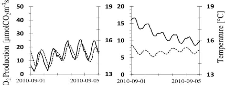
Furthermore, top soil CO2 production terms presented a larger amplitude
variation and phase shift in comparison with deeper CO2 sources. For
exam-ple, as represented during dry days at figure 2, the CO2 production terms
simulated in layers between 5 and 10 cm depth presented a larger amplitude variation than those simulated between 20 and 25 cm depth. During dry days, we can relate such results to temperature measurements. Actually, the amplitude variation and the phase of production terms presented the same general behavior as the temperature measured in each layer.
The long term average of δ13P calculated on the soil profile is -27.4‰.
This is consistent with values reported in the literature. In comparison, the long term averages of measured and simulated δ13Fs are respectively -27.28
and -27.31‰. It means that δ13P and δ13Fs were nearly the same over period
of few days, showing that the steady state assumption (flux=production) is -30 -26 -22 0 4 8 2010-08-27 2010-09-01 2010-09-06 2010-09-11
C
O
2F
lu
x
[
µ
m
o
l
C
O
2m
-2s
-1]
δ
1 3F
(
‰
)
valid with relatively long time integration. Further analyses are currently on progress.
Figure 2 : Left Graph: Solid line represents CO2 production in the layer between 5-10 cm depth and dotted line the temperature measured in that layer. Right Graph: Solid line represents CO2 production in the layer between 20-25 cm depth and dotted line the temperature measured in that layer.
CONCLUSIONS
The simulations of surface CO2 flux and its isotopic signature are globally
consistent with the chamber measurements, especially during dry days. However, the δ13Fss presents larger amplitude of variation than the chamber
measurements. The dynamic and the distribution of production terms can be related respectively to climatic and soil variables. The isotopic composi-tion of produccomposi-tion calculated on the soil profile is consistent with values reported in the literature.
REFERENCES
Cerling, T. E., Solomon, D. K., Quade, J., & Bowman, J. R. (1991). On the isotopic composition of carbon in soil carbon dioxyde. Geochimica and Cosmochimica Acta ,
5, 3403-3405.
Ekblad, A., Boström, B., Holm, A., & Comstedt, D. (2005). Forest soil respiration rate and 13δC is regulated by recent above ground weather conditions. Oecologia , 143, 136-142.
Fang, C., & Moncrieff, J. B. (1999). A model for soil CO2 production and transport 1: Model development. Agricultural and Forest Meteorology , 95, 225-236.
Goffin, S., Longdoz, B., & Aubinet, M. (2011). Apport de l'approche multicouche et du signal isotopique pour la compréhension de la respiration du sol en écosystème forestier. Biotechnology, Agronomy, Society and Environment , 15 (4), 575-584. Kodama, N., Barnard, R. L., Salmon, Y., Weston, C., Ferrio, J. P., Holst, J., et al.
(2008). Temporal dynamics of the carbon isotope composition in a Pinus sylvestris stand: from newly assimilated organic carbon respired carbon dioxyde. Oecologia ,
156, 737-750.
Luo, Y., & Zhou, X. (2006). Soil respiration and the environment. Academic Press, Elsevier édition.
Maier, M., Schack-Kirchner, H., Hildebrand, E., & Holst, J. (2010). Pore-space CO2 dynamics in a deep, well-aerated soil. Eur. J Soil Sci. , 877-887.
Marron, N., Plain, C., Longdoz, B., & Epron, D. (2008). Seasonal and daily time course of the 13C composition in soil CO2 efflux recorded with a tunable diode laser spectrophotometer (TDLS). Plant Soil , 318, 137-151.
Moyes, A. B., Gaines, S. J., Siegwolf, R. T., & Bowling, D. R. (2010). Diffusive fractionation complicates isotopic partitioning of autotrophic and heterotrophic sources of soil respiration. Plant, Cell and Environment , 33, 1804-1819.
13 16 19 0 10 20 30 40 50 2010-09-01 2010-09-05 C O2 P ro du ct io n [µ m ol C O2 m -3s -1] 13 16 19 0 5 10 15 20 2010-09-01 2010-09-05 T em pe ra tu re [° C ]