Spectroscopic binaries as observed by the future Gaia space mission

Spectroscopic binaries as observed by the future Gaia

space mission

Yassine Damerdji, Ludovic Delchambre, Thierry Morel, Eric Gosset, Gregor Rauw

Institut d’Astrophysique et de G´eophysique, Universit´e de Li`ege, Belgium

Abstract: The future Gaia satellite will observe a large number of stars through its three main channels: astrometric, photometric and, for the brightest stars, spectroscopic. The satellite is equipped with the RVS spectrograph, which will provide medium-resolution spectra over a small wavelength range. These spectra should allow us to identify stars exhibiting a composite spectrum, either because of a chance alignment or a true binarity. We discuss the various aspects related to the data treatment of the binary candidates and describe the algorithms that are intended to be included in the processing pipeline.

1

Introduction

The aim of the ESA Gaia mission is to chart the Milky Way in its three dimensions. The Gaia astro-metric data will provide star positions, proper motions and parallaxes with unprecedented accuracy. The Radial Velocity Spectrograph (hereafter RVS) will provide the third dimension by measuring ra-dial velocities (RVs) using medium-resolution spectra. The characterization of the stellar populations (metallicity, age, masses) will also be made possible thanks to the on-board photometric capabili-ties. A census of about 1% of the galactic stellar population will be achieved by observing about one billion stars down to V = 20 mag during the 4 years of the mission (e.g., Mignard & Drimmel 2007). The data processing will be defined and performed under the responsibility of the Data Processing and Analysis Consortium (DPAC), which is split into 9 Coordination Units (hereafter CUs). Each CU is in turn divided into several Development Units (hereafter DUs). We are in charge of DU434, which will derive SB1 and SB2 Keplerian solutions for the candidate spectroscopic variables in the framework of the Non Single Stars branch of CU4 (‘Object Processing’). These candidates are either identified by CU6/CU7 (variability detection using RVs obtained within CU6) or by CU8 (stellar classification identifying binary stars using photometric data).

After a description of the specifications of the Gaia RVS experiment, we discuss the algorithms developed for the determination of the orbital parameters and their performance (both deterministic and non deterministic methods have been tested). Finally, we present the current results and discuss our efforts to improve them.

2

RVS specifications

The RVS radial velocities are derived by DPAC/CU6/DU650 (Single Transit Analysis) using single and double star cross-correlation and chi-square minimization techniques (e.g., Tonry & Davis 1979;

Table 1: Typical RVS radial velocity error bars (1σ) for single stars (in km s−1), as a function of the magnitude and spectral type (Viala et al. 2010).

Spectral type V = 6 V = 9 V = 12 V = 14

G5 V 0.4 2 5 15

B5 V 3 10 30

-Zucker & Mazeh 1994). Each observed spectrum in the RVS spectral range (846–874 nm; chosen to cover the calcium triplet) is cross-correlated with one or two combined synthetic spectra convolved with the instrumental Line Spread Function.

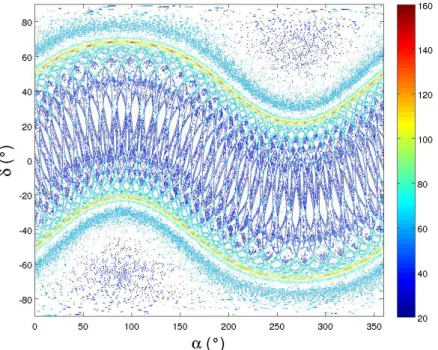
Figure 1 shows that the stars will transit in the RVS field of view on average about 50 times during the mission with values ranging from a minimum of 15 to a maximum of 161 observations.

Figure 1: Number of RVS transits in celestial coordinates. The median and mean values are 50 and 51.8, respectively.

Because of the lack for OB stars of metallic lines in the RVS spectral range compared to cooler stars (FGK types), the RV measurements will be much less accurate in this case (besides being more elegant, cross-correlation based algorithms are much more accurate than classical line fit functions because they take all the spectral lines into account). This is illustrated in Table 1, which shows the expected accuracies for a solar-like (G5 V) and a B5 V star.

3

Algorithms

The time series of RVs will be received from DPAC/CU6. They have to be cleaned from inconsistent measurements before starting their processing. The second step consists in searching for a periodicity in the remaining time series. Once this is achieved, an approached orbital solution can be obtained, which is then refined through a global minimization scheme. The final step is to test whether the

obtained eccentric orbit is significant against a circular one. The SB1/SB2 data processing pipeline is mainly composed of 7 sub-pipelines:

• Data cleaning: all bad/unphysical measurements are removed. A check is made to ensure that the remaining data are suitable for further processing.

• Period search: a period is searched using both the time series of RVs and the photometric periodicities provided by CU7. Many algorithms have been tested. We use the fit of a simple sine function in the time or phase space (Heck, Manfroid & Mersch 1985) to preselect the 100 most probable periods. Vr1 and |Vr2 − Vr1| are presently used for the SB1 and SB2 cases,

respectively.

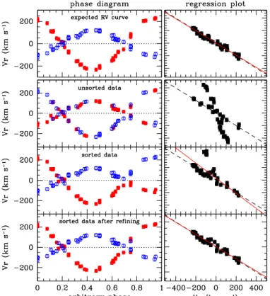
• Sorting of SB2 data: it is expected that the input velocity data will not necessarily be sorted (i.e., a given velocity will not be assigned either to the primary or to the secondary) because of a confusion in the identification of the spectral types during the computation of the RVs. The procedure used to assign the radial velocities to each binary component is illustrated in Fig.2. • Determination of the best period and derivation of the approached orbital solution. Many

al-gorithms have been tested (e.g., Russell 1902; Lehmann-Filh`es 1894; Monet 1979). We finally decided to use the method proposed by Zechmeister & K¨urster (2009) consisting in a fit of a simple sine function in the true anomaly domain.

• Derivation of the final orbital solution using a Levenberg-Marquardt minimization. We use Sterne (1941) and Schlesinger (1910) minimization schemes for low (e < 0.03) and high ec-centricity solutions, respectively.

• Test the final eccentric solution against the circular one using the test proposed by Lucy & Sweeney (1971).

• The steps (2) and (4) above may be replaced by a genetic algorithm (Haupt & Haupt 2008) com-bined with Zechmeister & K¨urster’s Keplerian periodogram. The optimization of the genetic algorithm parameters has to be performed beforehand.

4

Results

The algorithms described above have been tested on purely synthetic time series of RVs. Given the satellite scanning law and the design of the RVS focal plane, 8 sets of 120, 000 RV curves have been simulated, each corresponding to a given number of measurements and noise level. The grid of parameters is as follows:

• α = 0◦_{, δ = −90}◦ _{(this defines one typical but representative sampling law).}

• The number of measurements is 20 or 40.

• The Gaussian noise levels considered are: 0, 15, 30 and 45 km s−1_.

• Each set contains a logarithmic grid of 50 periods between 0.2 and 2000 days. • Each set contains a linear grid of 20 eccentricities between 0 and 0.95.

• Each set contains a linear grid of 12 longitudes of periastron between 0◦_{and 180}◦_{(for the other}

Figure 2: Illustration of the iterative method used to sort the SB2 velocities. The first panel illustrates the true RV curve while the second panel gives the observed wrongly attributed RVs. The open blue and red filled points corspond to the primary and secondary, re-spectively. The sorting is performed in two steps. The velocities folded in a phase diagram are first assigned to each com-ponent based on the identification of the nodes (velocities of the two components both roughly equal to the center-of-mass velocity of the system) in the RV curve (third panels from top). Second, the out-liers that are likely not properly assigned after the first step are iteratively identi-fied using a sigma-clipping algorithm in the (Vr1, Vr2) plane and their

identifica-tion permuted (bottom panels).

• Ten noise realisations are made for each combination of period, eccentricity and longitude of periastron.

• The semi amplitude and systemic velocity of all simulated curves are 100 and 0 km s−1

respec-tively.

• For the genetic algorithm, the settings are as follows: selection type = ROULETTE, mutation rate = 0.15, population size = 1000, number of iterations = 1000 and elite number = 20. Figure 3 shows the period search performances in the SB1 case for the deterministic (8 leftmost panels) and genetic algorithms (8 rightmost panels). As expected, the period is more frequently recov-ered when the number of measurements increases and/or the noise level decreases. The performance of the two algorithms is poor for very noisy data, although the genetic algorithm performs slightly better in this case. Satisfactory results are obtained for both algorithms for RV curves with 40 mea-surements. Figure 4 shows the performances for the refined eccentricities (without Lucy’s correction) for the deterministic (8 leftmost panels) and genetic algorithms (8 rightmost panels). The determin-istic algorithm is 15 times faster than the genetic algorithm but seems to be more sensitive to noise. This may be due to the limitations imposed by the user to the genetic algorithm to limit the execution time.

We are planning to test pattern recognition algorithms to determine the approached orbital solution using the folded RV curves. This study will be described in a future paper.

Acknowledgements

0 20 40 60 80 N_obs = 20 σ = 0km/s

Period recovery rate (%)

N_obs = 20 σ = 15km/s N_obs = 20 σ = 30km/s N_obs = 20 σ = 45km/s 0 0.2 0.4 0.6 0.8 0 20 40 60 80 N_obs = 40 σ = 0km/s

Period recovery rate (%)

e real 0 0.2 0.4 0.6 0.8 N_obs = 40 σ = 15km/s e real 0 0.2 0.4 0.6 0.8 N_obs = 40 σ = 30km/s e real 0 0.2 0.4 0.6 0.8 1 N_obs = 40 σ = 45km/s e real 0 20 40 60 80 N_obs = 20 σ = 0km/s

Period recovery rate (%)

N_obs = 20 σ = 15km/s N_obs = 20 σ = 30km/s N_obs = 20 σ = 45km/s 0 0.2 0.4 0.6 0.8 0 20 40 60 80 N_obs = 40 σ = 0km/s

Period recovery rate (%)

e real 0 0.2 0.4 0.6 0.8 N_obs = 40 σ = 15km/s e real 0 0.2 0.4 0.6 0.8 N_obs = 40 σ = 30km/s e real 0 0.2 0.4 0.6 0.8 1 N_obs = 40 σ = 45km/s e real

Figure 3: Period search performances for the deterministic (8 leftmost panels) and genetic algorithms (8 rightmost panels) as a function of orbital eccentricity. See text for the description of the input data. The genetic algorithm seems to be less sensitive to noise than the deterministic one.

0 0.2 0.4 0.6 0.8 1 N_obs = 20 σ = 0km/s erefined N_obs = 20 σ = 15km/s N_obs = 20 σ = 30km/s N_obs = 20 σ = 45km/s 0 0.2 0.4 0.6 0.8 0 0.2 0.4 0.6 0.8 N_obs = 40 σ = 0km/s erefined e real 0 0.2 0.4 0.6 0.8 N_obs = 40 σ = 15km/s e real 0 0.2 0.4 0.6 0.8 N_obs = 40 σ = 30km/s e real 0 0.2 0.4 0.6 0.8 1 N_obs = 40 σ = 45km/s e real 0 0.2 0.4 0.6 0.8 1 N_obs = 20 σ = 0km/s erefined N_obs = 20 σ = 15km/s N_obs = 20 σ = 30km/s N_obs = 20 σ = 45km/s 0 0.2 0.4 0.6 0.8 0 0.2 0.4 0.6 0.8 N_obs = 40 σ = 0km/s erefined e real 0 0.2 0.4 0.6 0.8 N_obs = 40 σ = 15km/s e real 0 0.2 0.4 0.6 0.8 N_obs = 40 σ = 30km/s e real 0 0.2 0.4 0.6 0.8 1 N_obs = 40 σ = 45km/s e real

Figure 4: The distribution of the refined orbital eccentricities (without Lucy’s correction) for the deterministic (8 leftmost panels) and genetic algorithms (8 rightmost panels) as a function of orbital eccentricity. See text for the description of the input data. Also in this case, the genetic algorithm seems to be less sensitive to noise than the deterministic one. The line on each panel shows the one-to-one aimed at relationship .

.

References

Heck, A., Manfroid, J. & Mersch, G. 1985, A&AS, 59, 63. Lehmann-Filh`es, R. 1894, AN, 136, 17.

Lucy, L.B. & Sweeney, M. A.,1971, AJ, 76, 544.

Mignard, F. & Drimmel, R. (eds), 2007, DPAC Proposal for the Gaia Data Processing, Gaia DPAC Technical note, GAIA-CD-SP-DPAC-FM-030

Monet, D.G. 1979, ApJ, 234, 275.

Haupt, R.L. & Haupt, S.E 1998, in Practical genetic algorithms, 2nd ed., ISBN 0-471-45565-2., 27, 150 Russell, H.N. 1902, ApJ, 15, 252.

Schlesinger, F. 1910, Pub. Allegheny Obs. (Pittsburgh), 1, 33. Sterne, T.E. 1941, Proc. Nat. Acad. Sc. USA, 27, 175. Tonry, J. & Davis, M. 1979, AJ, 84, 1511.

Viala, Y., Blomme, R., Fr´emat, Y., et al. 2010, WP650 Software Test Plan and Verification Report - Single Transit Analysis (Cycle 6), GAIA-C6-SP-OPM-YV-007-1.

Zechmeister, M. & K¨urster, M. 2009, A&A, 496, 577. Zucker, S. & Mazeh, T. 1994, ApJ, 420, 806.