HAL Id: hal-01206848
https://hal.archives-ouvertes.fr/hal-01206848
Submitted on 1 Oct 2015
HAL is a multi-disciplinary open access
archive for the deposit and dissemination of
sci-entific research documents, whether they are
pub-lished or not. The documents may come from
teaching and research institutions in France or
abroad, or from public or private research centers.
L’archive ouverte pluridisciplinaire HAL, est
destinée au dépôt et à la diffusion de documents
scientifiques de niveau recherche, publiés ou non,
émanant des établissements d’enseignement et de
recherche français ou étrangers, des laboratoires
publics ou privés.
Optimal General Simplification of Scalar Fields on
Surfaces
Julien Tierny, David Guenther, Valerio Pascucci
To cite this version:
Julien Tierny, David Guenther, Valerio Pascucci. Optimal General Simplification of Scalar Fields
on Surfaces. Topological and Statistical Methods for Complex Data, 2015, 978-3-662-44900-4.
�hal-01206848�
Abstract We present a new combinatorial algorithm for the optimal general topo-logical simplification of scalar fields on surfaces. Given a piecewise linear (PL) scalar field f , our algorithm generates a simplified PL field g that provably ad-mits critical points only from a constrained subset of the singularities of f while minimizing the distance || f − g||∞for data-fitting purpose. In contrast to previous
algorithms, our approach is oblivious to the strategy used for selecting features of interest and allows critical points to be removed arbitrarily and additionally mini-mizes the distance || f − g||∞in the PL setting. Experiments show the generality of
the algorithm as well as its time-efficiency, and demonstrate in practice the mini-mization of || f − g||∞.
1 Introduction
As scientific data-sets become more intricate and larger in size, advanced data anal-ysis algorithms are needed for their efficient visualization. For scalar field visualiza-tion, topological analysis techniques have shown to be practical solutions in various contexts by enabling the concise and complete capture of the structure of the input data into high-level topological abstractions such as contour trees [8, 9, 6], Reeb graphs [22, 25], or Morse-Smale complexes [18, 17]. Moreover, important advances
Julien Tierny
CNRS LTCI; Telecom ParisTech, 46 Rue Barrault, 75013 Paris, France, e-mail: [email protected]
David G¨unther
Institut Mines-Telecom; Telecom ParisTech; CNRS LTCI, 46, Rue Barrault, 75013 Paris, France, e-mail: [email protected]
Valerio Pascucci
SCI Institute, University of Utah, 72 S Central Campus Dr., Salt Lake City, UT 84112, USA, e-mail: [email protected]
have been made regarding the analysis of topological noise with the formalism of topological persistence [12], which enabled their multi-resolution representations and consequent progressive data explorations. However, the notion of feature is application-dependent. Using persistence to prioritize topological cancellations can be inappropriate for selecting features of interest in many scenarios (depending on the characteristics of the noise). For this reason, users often employ ad-hoc feature identification strategies that combine several criteria to determine which topological cancellations should be considered signal or noise [9]. While established simplifi-cation schemes produce multi-resolution representations of the topological abstrac-tions, they do not focus on generating an actual simplification of the underlying scalar field. However, simplifying the field before any analysis can be beneficial in a number of applications [26].
In this paper, we present a new combinatorial algorithm which generalizes and extends previous work on topological simplification of scalar fields [4, 26]. Given a scalar field f , our algorithm generates a simplified function g that provably ad-mits only critical points from a constrained subset of the singularities of f while strictly minimizing || f − g||∞ for data-fitting purposes. Bauer et al. [4] presented
such an optimal algorithm in the discrete Morse theory setting for the special case of persistence-driven simplifications. In this paper, we generalize this work to piece-wise linear (PL) scalar fields, which are commonly used in visualization software. In contrast to prior work [13, 3, 4], the proposed simplification scheme works with an arbitrary – not necessarily persistence-based – selection of singularities while still minimizing || f − g||∞. We illustrate this in several experiments which also show
empirically the optimality of the proposed algorithm.
1.1 Related work
The direct simplification of scalar fields given topological constraints is a subject that has only recently received attention. Existing techniques can be classified into two (complementary) categories.
Numerical approaches aim at approximating a desired solution by solving par-tial differenpar-tial equations, where a subset of the input singularities are used as topo-logical constraints while smoothness constraints are often used to enforce geometri-cal quality. The first work in this direction was presented by Bremer et al. [5], where simplified Morse-Smale complexes are used to guide an iterative and localized sim-plification of the field based on Laplacian smoothing. In the context of geometry processing, approaches have been presented for the computation of smooth Morse functions with a minimal number of critical points [21, 16]. Patan`e et al. [23] pre-sented a general framework for the topology-driven simplification of scalar fields based on a combination of least-squares approximation and Tikhonov regulariza-tion. Weinkauf et al. [27] improved the work by Bremer et al. [5] with bi-Laplacian optimization resulting in smoother (C1) output fields.
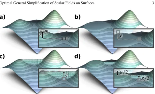
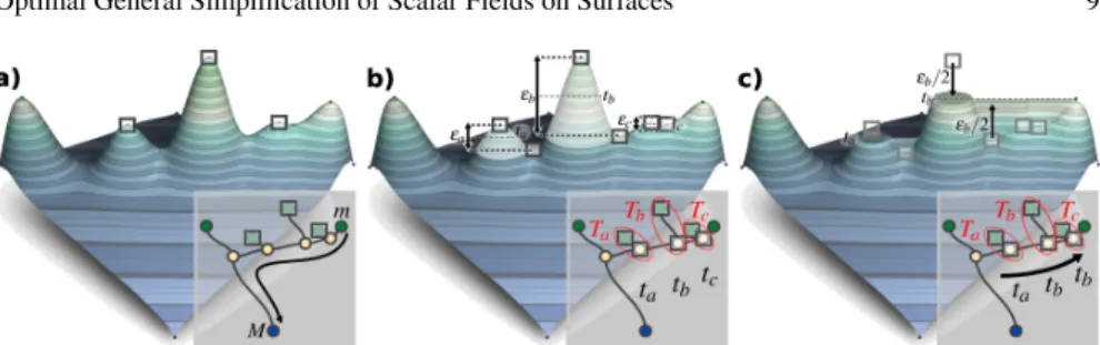
Fig. 1 Removing a maximum-saddle pair (m, s) from a scalar field f such that | f (m) − f (s)| = ε (a). A strategy based on flattening [26] (b) will lower m down to the level of s, yielding || f − g||∞=
ε . A strategy based on bridging [13] (c) will lift s up to the level of m, yielding || f − g||∞= ε. A
strategy based on a combination of the two [4] (d) will lower m halfway down to the level of s while lifting s halfway up to the level of m, yielding a minimized infinity norm || f − g||∞= ε/2.
However, one of the biggest challenge of these approaches is the numerical in-stability in the optimization process. This may create additional critical points in the output preventing it from strictly conforming to the input constraints. Additionally, the overall optimization process might be computationally expensive resulting in extensive running times.
Combinatorial approaches aim at providing a solution with provable correct-ness that is not prone to numerical instabilities. In a sense, they can be complemen-tary to numerical techniques by fixing possible numerical issues as a post-process.
Edelsbrunner et al. introduced the notion of ε-simplification [13]. Given a target error bound ε, the goal of their algorithm is to produce an output field everywhere at most ε-distant from the input such that all the remaining pairs of critical points have persistence greater than ε. Their algorithm can be seen as an extension of early work on digital terrain [24, 1] or isosurface processing [7], where the Contour Tree [8] was used to drive a flattening procedure achieving similar bounds. Attali et al. [3] and Bauer et al. [4] presented independently a similar approach for ε-simplification computation. By locally reversing the gradient paths in the field, the authors show that multiple persistence pairs can be cancelled with only one procedure.
However, these approaches admit several limitations. Their input is a filtration [12] or a discrete Morse function [15]. Since many visualization software require a PL function, the output needs to be converted into the PL setting requiring a subdi-vision of the input mesh (one new vertex per edge and per face). However, such a subdivision might increase the size of the mesh by an order of magnitude which is
not acceptable in many applications. Also, they focus on the special case where the critical points are selected according to topological persistence. On the other hand, Tierny and Pascucci [26] presented a simple and fast algorithm which directly op-erates on PL functions enabling an arbitrary selection of critical points for removal. However, this approach does not explicitly minimize the norm || f − g||∞.
1.2 Contributions
As illustrated in Figure 1, several strategies can be employed to remove a hill from a terrain (i.e. to remove a critical point pair from a function). In the context of persistence-driven simplification, tight upper bounds for the distance || f − g||∞have
been shown [10]. The algorithm by Bauer et al. [4] achieves these bounds in the dis-crete Morse theory setting. In this paper, we make the following new contributions: • An algorithm that achieves these bounds for the PL setting;
• An algorithm that minimizes the distance || f − g||∞in the case of general
sim-plifications (where the critical points to remove are selected arbitrarily).
2 Preliminaries
This section briefly describes our formal setting and presents preliminary results. An introduction to Morse theory can be found in [19].
2.1 Background
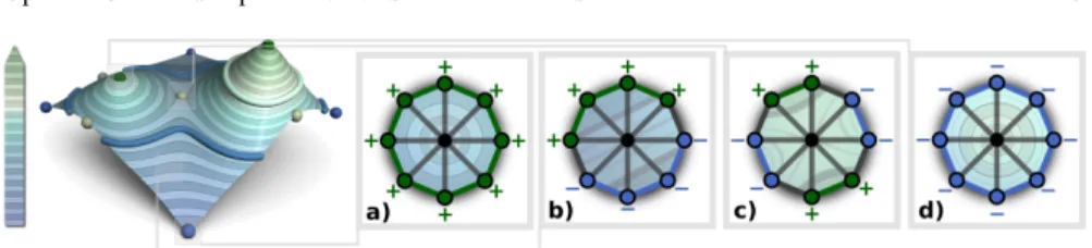
The input to our algorithm is a piecewise linear (PL) scalar field f :S → R defined on an orientable PL 2-manifoldS . It has value on the vertices of S and is linearly interpolated on the simplices of higher dimension. Critical points of PL functions can be classified with simple and inexpensive operations (Fig. 2). The star St(v) of a simplex v is the set of simplices σ that contain v as a face. The link Lk(v) of a simplex v is the set of simplices in the closure of the star of v that are not also in the star: Lk(v) = St(v) − St(v). The lower link Lk−(v) of v is the subset of Lk(v) containing only simplices with all their vertices lower in function value than v: Lk−(v) = {σ ∈ Lk(v) ∀u ∈ σ : f (u) < f (v)}. The upper link Lk+(v) is defined by: Lk+(v) = {σ ∈ Lk(v) ∀u ∈ σ : f (u) > f (v)}.
Definition 1 (Critical Point). A vertex v ofS is regular if and only if both Lk−(v) and Lk+(v) are simply connected, otherwise v is a critical point of f .
If Lk−(v) is empty, v is a minimum. Otherwise, if Lk+(v) is empty, v is a maximum. If v is neither regular nor a minimum nor a maximum, it is a saddle.
Fig. 2 Scalar field on a terrain (left). A level set is shown in blue; a contour is shown in white. Vertices can be classified according to the connectivity of their lower (blue) and upper links (green). From left to right: a minimum (a), a regular vertex (b), a saddle (c), a maximum (d).
A sufficient condition for this classification is that all the vertices ofS admit distinct f values, which can be obtained easily with symbolic perturbation [14]. To simplify the discussion, we assume that all of the saddles of f are simple ( f is then a Morse function [19]), andS is processed on a per connected component basis.
The relation between the critical points of the function can be mostly understood through the notions of Split Tree and Join Tree [8], which respectively describe the evolution of the connected components of the sur- and sub-level sets. Given an isovalue i ∈ R, the sub-level set L−(i) is defined as the pre-image of the open interval (−∞, i] ontoS through f : L−(i) = {p ∈S f (p) ≤ i}. Symmetrically, the sur-level set L+(i) is defined by L+(i) = {p ∈S f (p) ≥ i}.
The Split TreeT+of f is a 1-dimensional simplicial complex obtained by
con-tracting each connected component of the sur-level set to a point. By continuity, two vertices vaand vbofS with f (va) < f (vb) are mapped to adjacent vertices inT+
if and only if for each vc∈S there holds f (vc) ∈ ( f (va), f (vb)):
• the connected component of L+( f (v
a)) which contains vaalso contains vb;
• the connected component of L+( f (v
c)) which contains vcdoes not contain vb.
By construction, a bijective map φ+:S → T+ exists between the vertices ofS
and those ofT+. Hence, for conciseness, we will use the same notation for a vertex
either inS or in T+. Maxima of f as well as its global minimum are mapped inT+
to valence-1 vertices, while saddles where k connected components of sur-level sets merge are mapped to valence-(k + 1) vertices. All the other vertices are mapped to valence-2 vertices. A super-arc (va, vb) [8] is a directed connected path inT+from
vato vbwith f (va) > f (vb) such that vaand vbare the only non-valence-2 vertices
of the path. The Join TreeT−is defined symmetrically by considering the sub-level
sets of f .
2.2 General simplification of scalar fields on surfaces
Definition 2 (General Topological Simplification). Given a field f :S → R with its set of critical pointsCf, we call a general simplification of f a scalar field g :
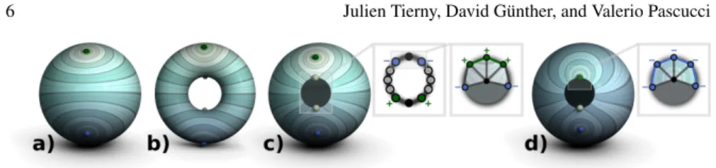
Fig. 3 Non removable critical points: (a) A global minimum and a global maximum have to be maintained for the field not to be constant. (b) 2 gSsaddles cannot be removed. (c),(d) Each bound-ary component has 2 non-removable global stratified extrema, which turn into non-removable sad-dles (c) or (possibly) exchangeable extrema (d).
In other words, a general simplification consists in constructing a close variant of the input field f from which a set of critical points has been removed. We call it optimalif it additionally minimizes the infinity norm || f − g||∞.
As described by Tierny and Pascucci [26], critical points can only be removed in extrema-saddle pairs. Hence, the removal of the saddles of f is completely de-pendent on the removal of its extrema. Note that there are also critical points that can not be removed due to the topology ofS (summarized in Fig. 3). We call them non-removablecritical points.
3 Algorithm
In this section, we present our new algorithm for the computation of optimal gen-eral simplifications. Given some input constraintsC0
g andCg2, i.e., the minima and
the maxima of g, our algorithm reconstructs a function g which satisfies these topo-logical constraints and minimizes || f − g||∞. Saddles are implicitly removed by our
algorithm due to their dependence on the minima and maxima removal.
To guarantee that the input field admits distinct values on each vertex, symbolic perturbation is used. In addition to its scalar value, each vertex v is associated with an integer offset O(v) initially set to the actual offset of the vertex in memory. When comparing two vertices (e.g., critical point classification), their order is dis-ambiguated by their offsetO if these share the same scalar value. Our new algorithm modifies the scalar values of the vertices (Sec. 3.1 to 3.3), while the algorithm by Tierny and Pascucci [26] is used in a final pass to update the offsets.
In the following sub-sections, we describe the caseCg0=C0
f (only maxima are
removed). The removal of the minima is a symmetrical process. We begin with the simple case of the pairwise critical point removal before we go into more complex and general scenarios addressing the removal of multiple critical points. The overall algorithm is summarized at the end of Sec. 3.3.
Fig. 4 (a) The set of flattening verticesF is identified from T+(transparent white). The set of
bridging verticesB is identified through discrete integral line integration (black curve). (b) The function values of each vertex ofF and B is updated to produce the simplified function.
3.1 Optimal pairwise removal
Let C2
g be equal to C2f\ {m} where m is a maximum to remove. As discussed in
[26], m can only be removed in pair with a saddle s where the number of connected components in the sur-level set changes (i.e. a valence-3 vertex inT+). Moreover, a
necessary condition for a critical point pair to be cancelled is the existence of a gra-dient path linking them [20]. In the PL setting, these are connected PL 1-manifolds called integral lines [11]. Thus, m can only be removed with a valence-3 vertex s∈T+that admits a forward integral line ending in m. Let S(m) be the set of all
saddles satisfying these requirements. Since integral lines are connected, m must belong to the connected components of L+( f (s)) which also contains s ∈ S(m). In T+, the saddles of S(m) are the valence-3 vertices on the connected path from m
down to the global minimum M of f .
To cancel a pair (m, s), one needs to assign a unique target value t to m and s. Since m is the only extremum to remove and m and s are the extremities of a monotonic integral line, we have:
|| f − g||∞= max(| f (m) − t|, | f (s) − t|) (1)
The optimal value t∗ which minimizes (1) is f (m) − | f (m) − f (s)|/2. Hence, we need to find the saddle s∗∈ S(m) that minimizes | f (m) − f (s)|. Since the saddles of S(m) lay on a connected path from m to M inT+, the optimal saddle s∗is the
extremity of the only super-arc containing m1.
LetF be the set of vertices of S mapped by φ+to the super-arc (m, s∗). Let
B be the forward integral lines emanating from s∗. The pair (m, s∗
) can then be removed by setting them to the value t∗such that no new critical point is introduced. This can be guaranteed by enforcing monotonicity on {F ∪ B}: Our algorithm assigns the target value t∗ to any vertex ofF which is higher than t∗and to any vertex ofB which is lower than t∗(see Fig. 4). Thus, given only one maximum to remove, our algorithm produces an optimal general simplification g.
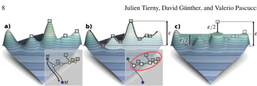
Fig. 5 Optimal simplification of a sub-tree Tk of the split treeT+. (a) A set of maxima
corre-sponding to the leaves of a connected sub-tree Tk is selected. (b) The optimal set of saddles to
remove can be identified with a simple traversal ofT+. Cancelling the critical points of Tkrequires
to process a function interval of ε = | f (m∗) − f (s∗)|, where m∗and s∗are respectively the highest
maximum and the lowest saddle of Tk. The set of candidate verticesF for flattening is directly
identified from Tk. The set of candidate vertices for bridgingB is identified by discrete integral
lines emanating from the saddles of Tk. (c) Updating the function values ofF and B yields an
infinity norm of ε/2: by lifting s∗up by ε/2 and by lowering m∗down by ε/2.
3.2 Optimal sub-tree removal
We call a sub-tree TkofT+a maximally connected sub-set ofT+such that: it
con-tains (a) k maxima of f to remove and (b) k valence-3 vertices ofT+, and that (c)
for all the valence-3 vertices si of Tkexcept the lowest, there exists no maximum
mto maintain such that si belongs to the connected path onT+from m down to
M (Fig. 5(a)). The optimal simplification of a sub-tree is a generalization of the previous case. By using the pairing strategy described in the previous sub-section, one can process the maxima of Tk in arbitrary order. The maxima are paired with valence-3 vertices ofT+and the corresponding super-arcs are removed. The
result-ing paired saddles will always be valence-3 vertices of Tkirrespectively of the order
in which the maxima are processed.
LetF be the pre-image of φ+ restricted to the super-arcs of Tk. LetB be the
forward integral lines emanating from the valence-3 vertices of Tk. By construction
{F ∪B} is a connected component, see Fig. 5(b), from which we aim to remove all the critical points. Similar as in the previous sub-section, these can be cancelled by assigning them a common target value t∗while enforcing monotonicity on {F ∪B} (no new critical point should be added).
For a given target value t, we have || f − g||∞= max(| f (m∗) − t|, | f (s∗) − t|) with
m∗and s∗being the highest maximum and the lowest saddle in Tk, respectively. The
target value t∗which minimizes || f − g||∞is then t∗= f (s∗) + | f (m∗) − f (s∗)|/2.
Thus, our algorithm assigns the target value t∗to any vertex ofF which is higher than t∗and to any vertex ofB which is lower than t∗.
All the sub-trees TkofT+can be identified with one breadth-first search traversal
of T+ seeded at the maxima to remove, in order of decreasing f value. In this
traversal, only the maxima to remove and the valence-3 vertices are admissible. Two connected components (seeded at the maxima to remove) can merge if there exists a super-arc between them. A connected components stops its growth if its number
Fig. 6 Optimal simplification of a sequence of sub-trees. While each sub-tree Tican be
individ-ually simplified at its optimal target value ti(b), monotonicity has to be enforced by selecting for
each sub-tree the maximum value among its own target value and its adjacent parent’s (c).
of maxima to remove equals the number of its valence-3 vertices. At the end of the traversal, each remaining component forms a maximally connected sub-tree Tk.
3.3 Optimal sub-tree sequence removal
In this sub-section, we finally describe the optimal simplification of a sequence of sub-trees (corresponding to the most general case, where maxima can be selected for removal arbitrarily).
For a given set of maxima to remove (Fig. 6(a)), the corresponding maximally connected sub-trees can be identified with the algorithm described in the previous sub-section. Moreover, it is possible to compute their individual optimal target val-ues {tk} that creates optimal simplifications of the sub-trees {Tk}. To guarantee the
monotonicity of the function, special care needs to be given to sub-trees that are adjacent to each other but separated by a super-arc, see Fig. 6(b).
Let T0and T1be two sub-trees such that s0and s1are the lowest valence-3 vertices
of T0and T1, respectively. Additionally, let s0and s1be connected by a super-arc
(s1, s0) with f (s1) > f (s0). Since T0 and T1 are adjacent yet distinct maximally
connected sub-trees, there exists at least one maximum m to preserve with f (m) > f(s1) > f (s0) such that s0and s1both belong to the directed connected path from m
down to the global minimum M of f , see Fig. 6. Hence, in contrast to the previous sub-section, monotonicity should additionally be enforced on the connected path on T+from m down to M.
LetF be the pre-image through φ+of the super-arcs of T0and T1 andB the
forward integral lines emanating from the valence-3 vertices of T0and T1. Since T0
and T1are adjacent, {F ∪B} is again a connected component on which g has to be
monotonically increasing. Two cases can occur:
1. t0< t1: Simplifying the sub-trees T0 and T1 at their individual optimal target
values t0and t1yields a monotonically increasing function on {F ∪ B}
2. t0> t1: Simplifying the sub-trees T0and T1at t0and t1would yield a decreasing
function, and hence introduce a new critical point on {F ∪ B}. (An example is given in Fig. 6(b) for the case T0= Tband T1= Tc). In this case, forcing T1to
use t0as a target value will correctly enforce monotonicity while not changing
the distance || f − g||∞2, see Fig. 6(c).
Hence, the optimal target value needs to be propagated along adjacent sub-trees to enforce monotonicity. To do so,T+is traversed by a breadth-first search
with increasing f value. When traversing a vertex s1, which is the lowest
valence-3 vertex of a sub-tree T1, the algorithm checks for the existence of a super-arc
(s1, s0) such that s0 is the lowest valence-3 vertex of a sub-tree T0. The optimal
target value t1is updated to enforce monotonicity: t1← max(t0,t1). Note that this
monotonicity enforcement among the target values does not change || f − g||∞.
Hence, an optimal simplification is guaranteed. In particular, || f − g||∞ will be
equal to | f (m∗) − f (s∗)|/2 with s∗and m∗being the lowest valence-3 and the high-est valence-1 vertex of the sub-tree T∗which maximizes | f (m∗) − f (s∗)|. In case of persistence-guided simplification, the simplified function g achieves the upper bound || f − g||∞= ε/2 with ε = | f (m∗) − f (s∗)|.
In conclusion, the overall algorithm for optimal simplification can be summa-rized as follows:
1. Identifying the sub-trees to remove (Sec. 3.2);
2. Enforcing monotonicity on the target values of each sub-tree (Sec. 3.3);
3. Cancelling each sub-tree to its target value with a combination of flattening and bridging (Sec. 3.1 and 3.2).
4. Running the algorithm by Tierny and Pascucci [26] as a post-process pass to disambiguate flat plateaus. This last pass is a crucial step which is mandatory to guarantee the topological correctness in the PL sense of the output.
The optimal simplification of the function given some minima to remove is obtained in a completely symmetric fashion by considering the Join TreeT−.
4 Results and Discussion
In this section, we present results of our algorithm obtained with a C++ implementa-tion on a computer with an i7 CPU (2.93GHz). In the following, the funcimplementa-tion range of f exactly spans the interval [0, 100] for all data-sets.
Computational complexity. The construction of the Split and Join Trees takes O(nlog(n)) + (n + e)α(n + e) steps [8], where n and e are respectively the number of vertices and edges inS and α() is an exponentially decreasing function (inverse of the Ackermann function). The different tree traversals required to identify the sub-trees to remove and to propagate the target values take at most O(nlog(n)) steps.
2 Since f (s
0) < f (s1) and t0> t1, then | f (s0) − g(s0)| = t0− f (s0) > t1− f (s1) = | f (s1) − g(s1)|.
Fig. 7 Comparison of the simplifications obtained with the algorithm proposed in [26] (a), || f − g||∞≤ ε) and our new algorithm (b), || f − g||∞≤ ε/2). Critical points are removed based on
topological persistence (the persistence threshold is ε). The topology of the fields is summarized with the inset Reeb graph for illustration purpose (input surface: 725k vertices).
Fig. 8 User driven simplification. The statistics of the simplification are shown in the grey frames for the flattening-only algorithm [26] (a) and for our new algorithm (b). The topology of the fields is summarized with the inset Reeb graph for illustration purpose (input surface: 75k vertices).
Updating the function values of the vertices for flattening and bridging takes linear time. The algorithm by Tierny and Pascucci [26] employed to post-process the offset values has been shown to achieve O(nlog(n)) performances in practice. Thus, the overall time-complexity of our algorithm is O(nlog(n)).
Persistence driven simplification is well understood in terms of infinity norm [10, 4]. We start our infinity norm evaluation with this setting to verify that our algorithm meets these expectations. As shown in Fig. 7, our algorithm improves the infinity norm in comparison with an algorithm solely based on flattening [26]. Given a persistence threshold ε, the output g generated by our algorithm satisfies
Fig. 9 An arbitrary sequence of pairwise optimal simplifications (a-d) does not necessarily pro-duce an optimal simplification. In this example, the global maximum is moved lower (d) than it would have been with our global algorithm (e). This results in a higher distance with regard to the infinity norm (d): || f − g||∞= 34.83, e): || f − g||∞= 26.02).
|| f − g||∞= ε∗/2 if the most persistent pair selected for removal has persistence
ε∗≤ ε.
General simplification aims for arbitrary critical point removal. Fig. 8 shows an example where the user interactively selected extrema to remove. Even in this general setting, our algorithm improved || f − g||∞by a factor of two compared to
[26].
Empirical optimality of our algorithm is illustrated in the last part of the experi-mental section. We provide practical evidence for the minimization of || f − g||∞. As
shown in Sec. 3.1 and in Fig. 1, an extremum-saddle pair can be removed optimally in a localized fashion. Hence, a general simplification can be achieved through a sequence of optimal pairwise removals for a given list of extrema to remove. How-ever, such a general simplification is not necessarily optimal as shown in Fig. 9. The
Terrain Fig. 6 Children Fig. 7 Dragon Fig. 8
Global algorithm 26.02 1.51 9.94
Pairwise sequences - Minimum 26.02 1.51 9.94 Pairwise sequences - Average 30.57 1.55 13.20 Pairwise sequences - Maximum 34.83 1.58 17.04
Table 1 Distance || f − g||∞obtained with our algorithm (top) and with sequences of optimal
pair-wise simplifications (bottom 3) on several data-sets for a given constrained topology. For simpli-fications based on pairwise sequences (bottom 3), the order of simplification of the critical point pairs is defined randomly (100 runs per data-sets).
examples. The minimum distance || f − g||∞obtained with this Monte-Carlo strategy
was never smaller than the distance obtained by our global algorithm. This illustrates that there exists no sequence of optimal pairwise removals that results in a smaller distance || f − g||∞than our algorithm. This shows empirically its optimality.
Limitations. Although our algorithm achieves the same time complexity as the flattening algorithm [26], our new algorithm is more computationally expensive, in practice (Figs. 7 and 8). This is due the use of the flattening algorithm in the final pass and the necessity of the Join and Split tree computations (which take longer than the flattening algorithm in practice).
In the general case, our algorithm may change the value of the maintained critical points after simplification. For instance, if the lowest minimum ofCg0 is initially higher than the highest maximum ofCg2, the algorithm will change their values to satisfy the topological constraints.
Finally, our algorithm provides strong guarantees on the topology of the output and on || f − g||∞at the expense of geometrical smoothness.
5 Conclusion
In this paper, we have presented a new combinatorial algorithm for the optimal general simplification of piecewise linear scalar fields on surfaces. It improves over state-of-the art techniques by minimizing the norm || f − g||∞in the PL setting and in
the case of general simplifications (where critical points can be removed arbitrarily). Experiments showed the generality of the algorithm as well as its time efficiency, and demonstrated in practice the minimization of || f − g||∞.
Such an algorithm can be useful to speed up topology analysis algorithms or to fix numerical instabilities occurring in the solve of numerical problems on surfaces (gradient field integration, scale-space computations, PDEs, etc.). Moreover, our algorithm provides a better data fitting than the flattening algorithm [26] since it minimizes || f − g||∞.
A natural direction for future work is the extension of this approach to volumet-ric data-sets. However, this problem is NP-hard as recently shown by Attali et al. [2]. This indicates that the design of a practical algorithm with strong topological guarantees is challenging.
Acknowledgements Data-sets are courtesy of AIM@SHAPE. This research is sup-ported and funded by the Digiteo unTopoVis project. The authors thank Hamish Carr for insightful comments and suggestions.
References
1. P. Agarwal, L. Arge, and K. Yi. I/O-efficient batched union-find and its applications to terrain analysis. In ACM Symp. on Comp. Geom., pp. 167–176, 2006.
2. D. Attali, U. Bauer, O. Devillers, M. Glisse, and A. Lieutier. Homological reconstruction and simplification in R3. In ACM Symp. on Comp. Geom., pp. 117–126, 2013.
3. D. Attali, M. Glisse, S. Hornus, F. Lazarus, and D. Morozov. Persistence-sensitive simplifica-tion of funcsimplifica-tions on surfaces in linear time. In TopoInVis Workshop, 2009.
4. U. Bauer, C. Lange, and M. Wardetzky. Optimal topological simplification of discrete func-tions on surfaces. Discrete and Computational Geometry, pp. 347–377, 2012.
5. P.-T. Bremer, H. Edelsbrunner, B. Hamann, and V. Pascucci. A topological hierarchy for functions on triangulated surfaces. IEEE Trans. on Vis. and Comp. Graph., 10:385–396, 2004. 6. P.-T. Bremer, G. Weber, J. Tierny, V. Pascucci, M. Day, and J. Bell. Interactive exploration and analysis of large-scale simulations using topology-based data segmentation. IEEE Trans. on Vis. and Comp. Graph., 17:1307–1324, 2011.
7. H. Carr. Topological Manipulation of Isosurfaces. PhD thesis, UBC, April 2004.
8. H. Carr, J. Snoeyink, and A. Ulrike. Computing contour trees in all dimensions. In Proc. of Symposium on Discrete Algorithms, pp. 918–926, 2000.
9. H. Carr, J. Snoeyink, and M. van de Panne. Simplifying flexible isosurfaces using local geo-metric measures. In Proc. of IEEE VIS, pp. 497–504, 2004.
10. D. Cohen-Steiner, H. Edelsbrunner, and J. Harer. Stability of persistence diagrams. Discrete and Computational Geometry, 37:103–120, 2007.
11. H. Edelsbrunner, J. Harer, and A. Zomorodian. Hierarchical Morse complexes for piecewise linear 2-manifolds. In ACM Symp. on Comp. Geom., pp. 70–79, 2001.
12. H. Edelsbrunner, D. Letscher, and A. Zomorodian. Topological persistence and simplification. Discrete & Computational Geometry, 28:511–533, 2002.
13. H. Edelsbrunner, D. Morozov, and V. Pascucci. Persistence-sensitive simplification of func-tions on 2-manifolds. In ACM Symp. on Comp. Geom., pp. 127–134, 2006.
14. H. Edelsbrunner and E. P. Mucke. Simulation of simplicity: a technique to cope with degen-erate cases in geometric algorithms. ACM Trans. on Graph., 9:66–104, 1990.
15. R. Forman. A user’s guide to discrete Morse theory. Adv. in Mathematics, 134:90–145, 1998. 16. Y. Gingold and D. Zorin. Controlled-topology filtering. Computer-Aided Design, 2006. 17. D. G¨unther, H. Peter-Seidel, and T. Weinkauf. Extraction of dominant extremal structures in
volumetric data using separatrix persistence. Comp. Graph. Forum., 2012.
18. A. Gyulassy, P.-T. Bremer, B. Hamann, and P. Pascucci. A practical approach to Morse-Smale complex computation: scalabity and generality. IEEE Trans. on Vis. and Comp. Graph. (Proc. of IEEE VIS), pp. 1619–1626, 2008.
19. J. Milnor. Morse Theory. Princeton University Press, 1963.
20. J. Milnor. Lectures on the H-Cobordism Theorem. Princeton University Press, 1965. 21. X. Ni, M. Garland, and J. Hart. Fair Morse functions for extracting the topological structure
of a surface mesh. ACM Trans. on Graph. (Proc. of ACM SIGGRAPH), 23:613–622, 2004. 22. V. Pascucci, G. Scorzelli, P. T. Bremer, and A. Mascarenhas. Robust on-line computation
of Reeb graphs: simplicity and speed. ACM Trans. on Graph. (Proc. of ACM SIGGRAPH), 26:58.1–58.9, 2007.
23. G. Patan`e and B. Falcidieno. Computing smooth approximations of scalar functions with constraints. Computers and Graphics, 33:399–413, 2009.
24. P. Soille. Optimal removal of spurious pits in digital elevation models. Water Resources Research, 40, 2004.
25. J. Tierny, A. Gyulassy, E. Simon, and V. Pascucci. Loop surgery for volumetric meshes: Reeb graphs reduced to contour trees. IEEE Trans. on Vis. and Comp. Graph. (Proc. of IEEE VIS), 15:1177–1184, 2009.
26. J. Tierny and V. Pascucci. Generalized topological simplification of scalar fields on surfaces. IEEE Trans. on Vis. and Comp. Graph. (Proc. of IEEE VIS), 2012.
27. T. Weinkauf, Y. Gingold, and O. Sorkine. Topology-based smoothing of 2D scalar fields with C1-continuity. Comp. Graph. Forum (Proc. of EuroVis), 29:1221–1230, 2010.

![Fig. 7 Comparison of the simplifications obtained with the algorithm proposed in [26] (a), ||f − g|| ∞ ≤ ε) and our new algorithm (b), || f − g|| ∞ ≤ ε/2)](https://thumb-eu.123doks.com/thumbv2/123doknet/11323078.282895/12.918.204.698.128.411/fig-comparison-simplifications-obtained-algorithm-proposed-new-algorithm.webp)

