Interval-Based Projection Method for Under-Constrained Numerical Systems

HAL Id: hal-00868023

https://hal.archives-ouvertes.fr/hal-00868023

Submitted on 1 Oct 2013

HAL is a multi-disciplinary open access

archive for the deposit and dissemination of

sci-entific research documents, whether they are

pub-lished or not. The documents may come from

teaching and research institutions in France or

abroad, or from public or private research centers.

L’archive ouverte pluridisciplinaire HAL, est

destinée au dépôt et à la diffusion de documents

scientifiques de niveau recherche, publiés ou non,

émanant des établissements d’enseignement et de

recherche français ou étrangers, des laboratoires

publics ou privés.

Interval-Based Projection Method for

Under-Constrained Numerical Systems

Daisuke Ishii, Alexandre Goldsztejn, Christophe Jermann

To cite this version:

Daisuke Ishii, Alexandre Goldsztejn, Christophe Jermann. Interval-Based Projection Method for

Under-Constrained Numerical Systems. Constraints, Springer Verlag, 2012, 17 (4), pp.432-460.

�hal-00868023�

(will be inserted by the editor)

Interval-Based Projection Method for

Under-Constrained Numerical Systems

Daisuke Ishii · Alexandre Goldsztejn · Christophe Jermann

Received: date / Accepted: date

Abstract This paper presents an interval-based method that follows the branch-and-prune scheme to compute a verified paving of a projection of the solution set of an under-constrained system. Benefits of this algorithm include anytime solv-ing process, homogeneous verification of inner boxes, and applicability to generic problems, allowing any number of (possibly nonlinear) equality and inequality constraints. We present three key improvements of the algorithm dedicated to projection problems: (i) The verification process is enhanced in order to prove faster larger boxes in the projection space. (ii) Computational effort is saved by pruning redundant portions of the solution set that would project identically. (iii) A dedicated branching strategy allows reducing the number of treated boxes. Ex-perimental results indicate that various applications can be modeled as projection problems and can be solved efficiently by the proposed method.

Keywords Numerical constraint programming · Interval analysis · Under-constrained systems·Projection method·Existentially quantified constraints

1 Introduction

Problems in various fields, such as control [11, 12, 16] and robotics [13, 22], amount to characterizing a set defined by anunder-constrained numerical constraint satis-faction problem (NCSP). For those under-constrained systems, which have generi-cally an uncountable infinity of solutions, aprojection of a solution set plays a key role in analyzing the system, especially when it becomes high dimensional. Indeed, not only resorting to projections is the only way for visualizing the solution set, but some projections can also convey a specific meaning; E.g., the projection on the pose parameters of the solutions to the kinematic equations of a robot represent D. Ishii

National Institute of Informatics, JSPS, Tokyo, Japan E-mail: dsksh@acm.org

A. Goldsztejn· C. Jermann

LINA, University of Nantes, CNRS, Nantes, France

thereachable workspaceof the considered robot, while the projection on the output parameters of the solutions of a command model represent its response range to the possible inputs. In many cases, a projected solution set has a positive hyper-volume1 even though the solution set before projection has a null hyper-volume.

Example 1 Consider the variables (x, y)∈[−2,3]×[−3,1] and the constraint (x+ cos 3y)2+ (y+ 1)2−1 = 0.

The solution set of this under-constrained NCSP is the 2D curve depicted in Figure 1(a). The projection of this solution set onto variablexis illustrated as the interval

xon thexaxis in the same figure.

When the constraints are polynomial, symbolic methods can solve a projection analytically (see e.g., [4]). However, symbolic methods can handle only very small systems because the size of the symbolic expressions involved grows exponentially with the number of variables and the degree of the constraints. Interval methods can handle non-polynomial constraints and they are able to compute a set of boxes (interval vectors) that approximates a projected solution set. An outer enclosure of the solution set can be computed using numerical constraint programming, but verification operators, like the interval Newton, are usually restricted to well-constrained systems. As an example, [19] is among the first work to provide an enclosure of the solutions of an under-constrained system of equations, but indeed it provides no verification. In order to be fully verified, a projected solution set has to be enclosed within two types of boxes: Inner boxes proved to be included inside the projected solution set; And (as small as possible)boundary boxespossibly containing points which are not the projection of any solution. The union of the inner and boundary boxes contains the projected solution set. The smaller the volume of the boundary boxes, the sharper the computed approximation.

The projection problem is difficult in general, and most existing interval meth-ods were proposed to deal with specific subclasses: Linear systems [24]; Inequality systems [21]; Systems where the different constraints do not share any projected variables [11, 12]. The first method able to deal with equality constraints that share projected variables is [5]. It consists of a standardBranchAndPrunealgorithm using the parametric Hansen-Sengupta operator as a verification test (i.e. Theorem 2 of this paper). This method was only applied to projection problems where projected variables domains do not need to be bisected (e.g. when the constraints depend linearly on these variables). In this case, Theorem 2 applies efficiently to verify the projection. However, this verification process becomes highly unstable as soon as the projected variables domains are bisected, which is necessary in general. This issue has already been tackled by following two different ways proposed in [6] and [7]: First, [6] proposes a specific two phase algorithm where a first phase computes an over approximation of the boundary of the projection using some necessary conditions related to critical points of projections, and uses connectivity analysis in order to identify pavings inside and outside the projection using this boundary over approximation. The second phase intends identifying part of the boundary over approximation that are in fact inside the projection by considering

1 _{The hyper-volume, also called Lebesgue measure, is the generalization to arbitrary}

- 1 0 1 2 -2 -1 0 x y x

(a) Exact projection of the solution set. (b) Solution with standard BranchAndPrune.

(c) Solution with the new verification process and search strategy.

(d) Solution with the new pruning technique.

Fig. 1 Sketch of the essential components of our BranchAndPrune method on a simple

pro-jection problem.

a perturbed problem. This second phase is critical since the boundary necessary condition is not sufficient, and the points inside the projection that verify the suf-ficient condition (called weak boundary points in [6]) can split the projection in several fake subcomponents. Although being the first method able to verify the projection of equality constraints sharing variables whose domains require split-ting, this method presents two main drawbacks: Tuning the precision of the first phase is very difficult, while the second phase is very sensitive to the output of the first phase, resulting in an algorithm quite difficult to use and tune in practice. In addition, it can only handle equality constraints, and it seems not possible to ex-tend it to problems including inequality constraints. The second method proposed in [7] tackles the instability of verification when projected variables domains are bisected using the so-called domain inflation technique which proved to be very efficient. It is however restricted to the computation of the direct image of set defined by inequalities through a vector-valued function, which does not require a

BranchAndPrunealgorithm since only the projected variables are bisected, resulting

in a simple bisection algorithm.

In this paper, instead of another specialized projection algorithm, we propose to use the successful paradigm ofBranchAndPrunealgorithms (Section 2.3) in order to tackle general projection problems (Section 3). While treating as general problems as the method in [6], this approach overcomes its disadvantages:

– BranchAndPrune algorithms are intrinsically anytime2 _{as they produce}

arbi-trarily sharp approximations of solution sets, the user being able to stop the computation when the desired accuracy of the approximation, or a resource (e.g., time) limit, is reached [2].

– When run with a sufficient precision, or enough computation time, no weak boundary box appears in this approach, which leads to a homogeneous inner approximation.

– Solving projection problems using a standardBranchAndPrunealgorithm allows fully benefiting from numerical constraint programming techniques, including a native treatment of inequality constraints.

Still, the standardBranchAndPrunealgorithm for under-constrained numerical constraint satisfaction problems is bound to behave poorly when used as it is for projection problems. Indeed, it will face difficulties for verifying inner boxes because it requires that the box to be verified contains a unique corresponding solution for each projected point. This will often be false due to the bisections employed during the search.

Example 2 Considering again the problem presented in Example 1, Figure 1(b) illustrates the result computed by the BranchAndPrune algorithm. The boxes in this figure form the set S, a paving of the solution set of the under-constrained NCSP. An enclosure of the projection is obtained by taking the union of all thex

component of these boxes, as shown on thexaxis. The thick boxes ofS are those whose projection is verified to be inner whereas the thin boxes are not verified. The inner approximation of the projection of the solution set is the union of thex

component of the verified boxes. As depicted in the figure, it is very poor in this example and consists of several disjoint parts. In fact, we can see that verified and non-verified boxes appear somehow arbitrarily in the solution set. This is typical of an inefficient verification procedure together with an unadapted search strategy. In theory, it is impossible to devise a perfect search strategy that would bi-sect the search space just where needed for the verification process to succeed everywhere. Hence, in order to devise a suitable BranchAndPrune algorithm for projection problems, we propose to enhance the verification mechanism so as to compensate the wrong bisections: Our verification method presented in Section 3.1 applies an inflation technique to the considered box, dynamically shifting the pa-rameters in order to match each of the projected points in the box. In addition,

ourBranchAndPrunealgorithm adopts a specific search strategy which avoids

un-necessary splitting and facilitates the verification process.

Example 3 Figure 1(c) presents the result of the BranchAndPrune algorithm that uses our verification method and search strategy on the problem introduced in Ex-ample 1. It shows that most of the boxes are verified thanks to our enhancements. The boxes that are not verified are too close to critical points of the projection, i.e., points where the solution set is orthogonal to the projection. No verification method could prove boxes enclosing such points.

Still, it appears much could be gained by considering the projection mechanism during the computation of the paving S. Indeed, as soon as a portion of the

projection has been verified to be inner, it becomes useless to pave additional parts of the solution set that would project identically. Hence the cylinder above the projection of a verified box can be used for pruning during the rest of the computation (Section 3.2).

Example 4 It is clear in Figures 1(b) and 1(c) that some redundant computations are performed because there are overlapping of up to 4 solutions within the pro-jection. Considering verified boxes as a mean of pruning redundant portions of the search space, we can obtain the much less verbose paving depicted in Figure 1(d). The paper is organized as follows: Section 2 introduces the necessary back-ground on NCSPs and recalls the genericBranchAndPrunealgorithm; Section 3 de-fines formally projection problems and details the adaptation of theBranchAndPrune

algorithm to these problems, in particular the new verification process (Section 3.1), the new pruning technique (Section 3.2) and the new search strategy (Section 3.3); Section 4 presents experimental evidences of the practical usefulness and perfor-mances of our method, especially in comparison to results from the literature; Section 5 concludes the paper.

2 Numeric Constraint Solving

Numeric constraint solving inherits principles and methods from discrete con-straint solving [23] and interval analysis [18]. Indeed, the specificity of the problems they address is that their variables take values in continuous subsets ofR. It is thus impossible to enumerate the possible assignments as classically done in discrete constraint solving. To overcome this situation, numeric constraint solvers resort to interval computations : Each variable takes an interval as a domain, representing the fact it can take any value within this interval. It is then possible to enumerate machine-representable interval assignments using the dichotomy principle of the

BranchAndPrunescheme.

The following subsection recalls the necessary definitions of interval analysis, the following one defines numeric constraint satisfaction problems and the one after presents the classicalBranchAndPrunealgorithm for numeric constraint solving.

2.1 Interval Analysis

The goal of interval analysis [18, 20] is to extend real computations to interval computations. It is based on the containment principle, i.e., intervals must be un-derstood as “any possible real value in the interval” and thus the result of interval computations must be intervals enclosing any possible result of the correspond-ing real computations. As a tool capable of handlcorrespond-ing rigorously uncertainties and computational errors, interval analysis has become a framework of choice for ver-ified floating-point computations on machines. Below are the basic concepts and notations from interval analysis used in this paper.

The notation of intervals in this paper conforms to the standard [14]. A (bounded)

interval a= [a, a] is a connected set of real numbers{b ∈R| a ≤ b ≤ a}.IR denotes the set of intervals. For an intervala,aandadenote the lower and upper bounds; widadenotes the width, i.e.,a−a; intadenotes the interior, i.e., the open interval

{b ∈R| a < b < a}; and midadenotes the midpoint, i.e., (a+a)/2. For intervalsa

andb, dist(a, b) denotes the hypermetric between the two, i.e., max(|a−b|, |a−b|), and a\ b denotes the set difference, i.e., {c ∈ R | c ∈ a, c /∈ intb}, which can also be represented as the union of at most two intervals. All these definitions are naturally extended to interval vectors.

Ad-dimensionalbox (or interval vector)ais a tuple ofdintervals (a1, . . . , ad).

IRd_{denotes the set ofd-dimensional boxes. For a real vectora∈R}d_{and a boxa∈}

IRd_{, we use the inclusion notation}

a∈ athat is interpreted as∀i∈{1, . . . , d}(ai∈ ai). A paving P is a set of boxes {a1, . . . , ak} such that all ai have the same

dimensiond. Boxes in a paving may overlap. We denote∪P the union of the boxes in a pavingP, i.e., the set{a ∈Rd | ∃ai∈P (a∈ ai)}.

For a function f :Rd →R, f :IRd→IR is called aninterval extension off if and only if it satisfies thecontainmentcondition:

∀a∈IRd _∀a∈a

(f(a)∈ f(a)).

This definition is generalized to function vectorsF:Rd→Re.

2.2 Numeric Constraint Satisfaction Problems

Anumeric constraint satisfaction problem(NCSP) is defined as a tripleP=⟨v, vInit, c⟩ that consists of

– a list of variables v= (v1, . . . , vd),

– an initial domain, in the form of a box, represented asvInit∈IRd, and

– a constraint cdescribed as

F(v) = 0∧ G(v)≥0,

where F :Rd →Rp andG:Rd →Rq, i.e., the constraint is a conjunction of equations3 _{and inequalities.}

Throughout the rest of the paper,d(resp.p,q) will denote the number of variables (resp. equations, inequalities) of the considered problem. Asolutionof an NCSP is an assignment of its variables ˜v∈ vInit that satisfies its constraints. Thesolution set Σ of an NCSP is the region withinvInit that satisfies its constraints:

Σ(P) :={v ∈ vInit | c(v)}.

An NCSP is said to beover-constrained whend < p(generically, its solution set is empty), well-constrained when d=p(generically, its solution set is discrete), and

under-constrained whend > p(generically, its solution set is continuous).

2.3 StandardBranchAndPrunefor NCSPs

TheBranchAndPrunealgorithm is the standard complete solving method in the

con-straint programming paradigm. It interleaves refutation phases, known as prune

Algorithm 1 BranchAndPrunealgorithm.

Input: NCSP⟨v, vInit, c⟩

Output: pair of lists of boxes (L, S) 1: L← {vInit} 2: S← ∅ 3: while¬Stop()do 4: v← Extract(L) 5: v← Prune(v) 6: if v̸=∅ then 7: if Prove(v)then 8: S← S ∪ {v} 9: else 10: L← L ∪ Branch(v) 11: end if 12: end if 13: end while 14: return (L, S)

asbranchoperation, that divide the search space into parts to be processed itera-tively. Algorithm 1 is a generic implementation of this scheme.

It takes as an input the problem to be solved and returns as an output a paving that distinguishes: Verified solutions in S, and unproven (or indiscernible) boxes inL. This implementation makes use of five abstract routines4:

– Stopdecides when the solving is completed. In numeric constraint solving it is usually implemented as a test on the precision of the boxes in L, but it can also involve a timeout check in an anytime solving context.

– Extract selects, at each iteration, the portion of the search-space to be pro-cessed. Together with the Branch operation, it defines the search strategy of the algorithm. In numeric constraint solving, it typically implements either a depth-first search (DFS), breadth-first search (BFS) or width-first search (WFS) strategy, respectively implemented by consideringLas a stack, a queue, or a priority queue ordered by the width of the contained boxes (i.e., the width of their largest intervals).

– Prune filters out inconsistent parts of the considered portion of the search-space, using various definitions of local and global consistencies. In numerical constraint solving, it typically removes only boundary portions of the con-sidered box in order to preserve domains represented as intervals (shaving). It usually makes use of local numerical consistencies like Hull or Box consis-tency [17, 25], or enhanced versions like MOHC [1], and global contractors like the interval Newton [7].

3 _{The vectorial equation F (v) = 0 stands for the system f}

1(v) = 0, . . . , fp(v) = 0, vectorial

inequalities being defined component-wise as well.

4 _{For the sake of clarity, the problemP and the lists L and S are supposed to be accessible}

– Prove verifies that the considered portion of the search-space is a solution of the problem5_{. Being a solution can take different meaning depending on the}

considered problem and the question asked. For instance, if the question is to find the real solution of a well-constrained NCSP, then it will generally im-plement a solution existence (and often uniqueness) theorem, e.g., Miranda, Brouwer or interval Newton [20], that guarantees that the considered box con-tains a (unique) real solution; on the other hand, if the question is to compute an inner paving of the continuous solution set of an under-constrained NCSP, then it will usually implement a solution universality test that guarantees that every real assignment in the considered box is a solution of the NCSP.

– Branchsplits the considered search-space into sub-parts that are inserted back into the list L of portions to be processed. In numeric constraint solving, it typically amounts to bisecting the considered box along one of its dimension. The choice of the dimension to be split, and the split point, are elements of the search strategy of the algorithm. In general, domains are split in a round-robin mode and at their midpoints.

3 Branch-and-Prune Algorithm for Projection Problems

A projection problem consists in computing the projection of the solution set of an under-constrained NCSP. More precisely, a projection problem is defined as an NCSPP = ⟨v, vInit, c⟩ and a partition of the variables v= (x, y) wherex andy

are of sizenandmrespectively. The variablesxandyare respectively called the projection scope and the projected variables. For commodity, the initial domain ofxis denotedxInitand that ofyis denotedyInit, hencevInit= (xInit, yInit). The solution to a projection problem is the projected solution set of its NCSP and is defined as

Σx(P) :={x ∈ xInit | ∃y ∈yInit (c(x, y))},

which is the projection of the solution setΣonto thexvariables.

We consider projection problems wherecis the conjunction ofpequality con-straints, where p≤ m, and arbitrarily many inequality constraints. This require-ment on the number of equality constraints ensures that the projected solution set generically has a dimension equal ton, i.e. it has a non-null hyper-volume. In this situation, one has to compute both an inner and an outer approximation of

Σx(P), therefore the output of Algorithm 1 specialized to projection problems has

the following interpretation:

∪Sx⊆ Σx(P)⊆ ∪(Lx∪ Sx), (1)

whereSx:={x | ∃y((x, y)∈ S)}is the projection onxof the boxes contained in

S, and Lx is defined similarly fromL.

In the following subsections, we show how the generic BranchAndPrune algo-rithm described in Algoalgo-rithm 1 has to be implemented in order to compute ef-ficiently pavings satisfying (1). In particular, the implementation of functions in Algorithm 1, i.e.,Prove(Subsection 3.1),Prune(Subsection 3.2) andBranch (Sub-section 3.3) dedicated to projection problems are defined below. These sub(Sub-sections

5 _{This routine is the main difference with the discrete variant of the BranchAndPrune where}

present techniques restricted to the well-constrained case (i.e., the number m of projected variables is equal to the numberpof equations). Their adaptation to the under-constrained case (i.e.,p < m) is presented in Subsection 3.4. Appendixes A and B provide the pseudo code that implements the subroutines ofBranchAndPrune.

3.1 Verification of Inner Boxes

This section describes how we implement Prove in Algorithm 1. The goal of our implementation is to verify that the processed box is projected striclty insideΣx.

More formally, it operates on a box (x, y) and tries to prove that ∀x ∈ x ∃y ∈

yInit (F(x, y) = 0). The verification process proposed here is based on a para-metric version of the well known Hansen-Sengupta operator: Indeed, the system

F(x, y) = 0 can be interpreted as a parametric system Fx(y) = 0 for which the

previous quantified proposition intends proving that it has a solution for every parameters values. We first recall the verification of solutions to nonparamet-ric systems of equations in Subsection 3.1.1. Then, we show that a parametnonparamet-ric Hansen-Sengupta operator can be used to prove∀x∈x ∃y ∈y(F(x, y) = 0), which is a sufficient condition for the first proposition sincey⊆ yInit; we also argue that such a verification process does not lead to convergent inner approximations. Fi-nally, we propose thedomain inflation technique dedicated to parametric systems of equations in Subsection 3.1.3.

3.1.1 Verification of Solutions to Nonparametric Systems

The Hansen-Sengupta operator is a computationally efficient version of the interval Newton operator defined as follows: LetF :Rm→Rm,F be an interval extension ofF,y∈IRm, ˜ybe any6 point iny,J be an interval enclosure of the Jacobian of

F ony, andC∈Rm×mbe any7 _{nonsingular matrix used as a preconditioner for}

J,

H(y) := ˜y+Γ(CJ ,−CF(˜y), y−y˜), (2) where

Γ(A, a, b) := (Diag−1A)(a−(OffDiagA)b)

with Diag−1Athe diagonal interval matrix whose diagonal entries are (Diag−1A)ii

= 1/aiiand OffDiagAthe interval matrix whose diagonal entries are null and

off-diagonal entries are (OffDiagA)ij=aij.

Note that this operator is defined only for systems that have exactly as many variables as equations. This requirement is mandatory for the application of inter-val Newton operators, and we discuss how to change under-constrained systems into well-constrained ones in Section 3.4. Note also that in this version of the operator, diagonal entries must be intervals that do not contain 0 otherwise the operator cannot be applied8. Finally, remark that contrarily to most forms found

6 _{Usually, ˜y := mid y.}

7 _{The preconditioning matrix is usually chosen as C := (mid J )}−1_{since it guarantees some}

good convergence properties while the approximate inversion is not too expensive for the systems of relatively small size usually handled by interval analysis.

8 _{An extended version of the operator handles general interval matrices but the existence}

in the literature, the result of the operator presented here is not intersected with the original boxy. Its interpretation is summarized by the following theorem:

Theorem 1 ([10, 20]) Let y ∈ IRm, F : Rm → Rm be a differentiable function. Then, every zero of F that belongs to y also belongs to H(y). Furthermore, F has a unique zero in H(y)if the following condition holds:

∅ ̸=H(y)⊆inty.

In other words, the Hansen-Sengupta prunes a box without losing any solution, and strict inclusion of the pruned box in the initial box guarantees the existence of a unique solution.

3.1.2 Verification of Solutions to Parametric Systems

The parametric Hansen-Sengupta operator is defined as follows: LetF(x, y) :Rn× Rm _→Rm_,

F be an interval extension of F, (x, y)∈ IRn+m, ˜y be any point in

y,Jy be an interval enclosure of the Jacobian of F on (x, y) with respect to the

m projected variables y, and C ∈ Rm×m be any nonsingular matrix used as a preconditioner forJy

Hx(y) := ˜y+Γ(CJy,−CF(x,˜y), y−y˜). (3)

Like its nonparametric version, this parametric Hansen-Sengupta operator is de-fined only for functions that have exactly as many components as variablesy, i.e., as many equations as existentially quantified variables.

The following theorem allows using the parametric Hansen-Sengupta as a ver-ification procedure for the projectionxof a box (x, y) to be included insideΣx.

Theorem 2 ([5]) Let(x, y)∈IRn+m, F(x, y) :Rn×Rm→Rm be a differentiable function. Then,∃(x, y)∈(x, y)such that F(x, y) = 0 implies y∈ Hx(y). Further-more,∀x∈x ∃y ∈Hx(y) (F(x, y) = 0)holds when:

∅ ̸=Hx(y)⊆inty

Proof Using the inclusion monotonicity of the interval arithmetic,Hx˜(y)⊆ Hx(y)

holds for an arbitrary ˜x∈ x. On the other hand,H˜x(y) is exactlyH(y) applied

to the function F(˜x,·). Theorem 2 then directly follows from the application of

Theorem 1. ⊓⊔

Figure 2(a) illustrates the successful application of Theorem 2: The plain box (x, y) is contracted to the dashed boxHx(y) (here vectorsx,y andF(x, y) have

only one component). The parametric Hansen-Sengupta allows strictly contracting the y variable domain, and hence proves ∀x ∈ x ∃y ∈ Hx(y) (F(x, y) = 0), which

proves thatx⊆ ΣxsinceHx(y)⊆ y ⊆ yInit.

Consider now the same situation but where the interval y is the half of the previous one. This is illustrated in Figure 2(b), where the failure of Theorem 2 is obvious: The quantified proposition ∀x ∈ x ∃y ∈ y (F(x, y) = 0) is now false, and accordingly the dashed box Hx(y) is not anymore strictly contained in the

0.4 0.5 0.6 0.7x 0.7 0.8 0.9 1.0 y f(x,y)= 0

(a) Case of success.

0.4 0.5 0.6 0.7 0.7 0.8 0.9 1.0 x y (b) Case of failure.

Fig. 2 Verification of boxes using the parametric Hansen-Sengupta.

projected variables domains have to be bisected to ensure the convergence of the computation9_.

This is dramatic for the success of the BranchAndPrune algorithm which is based on the hypothesis that the smaller the domains, the better the involved operators behave. Under this hypothesis, splitting fairly all domains usually entails the convergence ofBranchAndPrune. Oppositely, we meet here a situation where a smaller domain leads to the failure of the proving process which strongly impacts the efficiency and the convergence ofBranchAndPrune, as already illustrated on an example in Figure 1(b), page 3.

3.1.3 Domain Inflation Technique for Projection Problems

This key issue was addressed for a simpler class of problems in [7] by the so-called

domain inflation technique. The idea of domain inflation can be extended to pro-jection problems as follows: Given a box (x, y) to be processed by theProveroutine of theBranchAndPrune, instead of checking that the parametric Hansen-Sengupta is strictly contracting the domainy, we use the domainy as the starting point of a search for a new domainy∗for which the parametric Hansen-Sengupta operator will be strictly contracting. Then provided that the inflated domain is included inside the initial domain, i.e., y∗ ⊆ yInit, the verification x⊆ Σx succeeds.

Fig-ure 2(b) provides a hint for computingy∗: AlthoughHx(y) is not strictly included

in y, it is obviously a good candidate fory∗. Repeating this process leads us to consider the limit y∞ of the sequenceyk+1:=Hx(yk), withy0:=y. When this

sequence is convergent, its limit satisfiesy∞=Hx(y∞) and therefore definingy∗

by slightlyinflating y∞(i.e., increasing by a small percentage its widths) generally allows the parametric Hansen-Sengupta to be strictly contracting. For efficiency reasons, the slight inflation step is interleaved with the sequence computation so as to allow obtaining strict contraction of the parametric Hansen-Sengupta opera-tor the soonest. The algorithm that interleaves slight inflation and the parametric

9 _{Some specific classes of problems do not require splitting the projected variables y domains.}

In this case, the simple application of parametric existence theorems can be successful, see e.g. [5].

Hansen-Sengupta iteration is described in Appendix A where a dedicated stopping criterion allows stopping the sequence early when the parametric Hansen-Sengupta is strictly contracting or when the sequence is diverging.

This iterated parametric Hansen-Sengupta process together with the inflation technique succeeds in verifying the inner projected boxes in both Figures 2(a) and 2(b). Hence, it will typically allow verifying large portions of the projection during

theBranchAndPruneprocess, as shown on the example in Figure 1(c), page 3.

3.2 Pruning Methods

The BranchAndPrune algorithm we propose makes use of three different pruning

operations: general pruning methods implemented as thePruneroutine, and more specific ones implemented within theProveandExtractroutines.

ThePrunefunction in our algorithm can use any typical constraint propagation

mechanism (e.g.,AC3-like propagation) based on numerical contracting operators like BC3-revise or HC4-revise, that respectively enforce Box and Hull consisten-cies [3, 17]. This is a strength of our method to be able to make use of any pruning method that applies to standard NCSPs to address projection problems. See Al-gorithm 5 in Appendix B for the detail.

The goal of the Pruneroutine in our method is to quickly get rid of infeasible regions in order to be able to verify early large boxes. In particular, it might be counterproductive to spend a lot of time pruning a box that could be verified as is. For this reason, we simply use a cheap AC3-like propagation of HC4-revise operators in this work. Evaluating the effect of using more expensive pruning operators should be a future work since, as typically observed, stronger operators are sometimes required to address more difficult problems.

Still, it is possible to achieve strong pruning without incurring any extra cost for it by using smartly the method implemented in theProvefunction. Indeed, the box

Hx(y) computed during this routine, whether it was successfully verified or not,

can ultimately be intersected with the original box (x, y) to produce a reduced box. This reduction applies only to theyvariables however. The verification process we have described in Section 3.1 guarantees this reduced box contains all the solutions in the original box if any exists. Hence, by trying to verify each box in the process, we can also prune them with a strong consistency enforcing operator.

The BranchAndPrune algorithm we use computes a paving of the solution set

Σof an under-constrained NCSP, but we are only interested in its projectionΣx.

In this projection, several boxes from the computed paving may overlap, meaning several y values correspond to the samex value. This is undesirable because, to verify that any given point ˜x is inside the projected solution set, we need only verifying one box (x, y) where it belongs. In order to avoid unnecessary (and time-consuming) iterations of the algorithm, we thus propose to eliminate from any box to be treated all the portions whose projections correspond to already verified projections: for a box (x, y)∈ Land any verified box (x′, y′)∈ S, we can replace (x, y) by (x\x′, y) inL. This process can also be considered a pruning, except that it does not refute inconsistent portions of the search-space but avoids exploring redundant ones instead. We implement it in theExtractroutine ofBranchAndPrune

(see Algorithm 4). A positive side-effect is that the produced projection appears more regular since no two projected boxes overlap thanks to this process.

For efficiency reasons, the fact that boxes overlap in the projected space is not recomputed each time; it is maintained all along the BranchAndPrune algorithm as a neighboring relation: two boxes (x, y) and (x′, y′) inLare neighbors if their projections overlap with a non-null volume, i.e., intx∩ x′ ̸=∅. Hence, the list L

in BranchAndPrunestores pairs (v, N) of boxes v along with a setN of (pointers

to) neighboring boxesv′. Then, each time we prune (Line 5 of Algorithm 1) and split a box (Line 10 of Algorithm 1), the associated listN is updated.

This method is not only a pruning operation but also a branching one. Indeed, the result of the set differencex\x′is in general not a box, but can be represented as the union of various sets of boxes. In this case, all the resulting boxes must be pushed back into the listL. However, generating too many boxes as the result of this operation is counterproductive and can yield memory consumption problems. Still, it is possible to restrict the use of this method to reasonable cases, for instance when the result of the set difference is at most one box, i.e., the projectionx′covers completelyx(then (x, y) is entirely pruned) or it covers all thexdimensions but one (then the boundary of this dimension is reduced in (x, y). This is the technique we have implemented since it does not induce any additional memory issues.

Using these pruning techniques altogether allows obtaining inexpensively a reg-ular paving of the projection as already illustrated on the example in Figure 1(d).

3.3 Search Strategy Tweaking

In the implementation of theBranchprocedure ofBranchAndPrune, we can tweak the search strategy in several ways in order to accommodate the projection problem (see also Algorithms 6 and 7 in Appendix B). We have chosen to adapt only the variable selection strategy and leave the split-point strategy to its default setting: balanced bisection. Indeed, there is no obvious split-point strategy that could be applied to projection problems, while there is a natural difference between selecting

xoryvariables.

The variable selection strategy role is to select a component of a box vto be split (because the box could not be verified yet) in order to produce sub-boxes to be pushed back into list L(Line 10 of the BranchAndPrunealgorithm). Standard variable selection strategies for NCSPs areround-robin(RR),largest-first (LF) and

smear-splitting (SS) [15]. RR selects at each application of the Branch procedure the next variable in an arbitrarily fixed order, and loops over all the variables; LF always selects the variable with the largest domain; SS selects the variable whose splitting have the highest potential impact on future prune phases according to an analysis of the partial derivatives of all constraints w.r.t. this variable.

None of them are appropriate to handle projection problems. Indeed, in order to minimize the computation time, our method aims at treating as few boxes as possible. To this end, for each point ˜xin the projected solution setΣxwe want to

verify a single box (x, y) such that ˜x∈ x. For the verification process to succeed, the considered box must contain a single ˜y value for each possible ˜x value in it. Hence we need to split yvariables as much as necessary to separate multiple values, but not more if possible. The existing strategies do not distinguishxandy

variables and thus cannot minimize the computational effort to pave the projected solution set.

Unfortunately, no strategy can in general decide whetheryvariables are suffi-ciently split or not. Hence we propose a heuristic variable selection strategy, called the dynamic dual round-robin (DDRR), that relies on the other aspects of the al-gorithm in order to estimate whether it is still needed or not (Alal-gorithm 7). This strategy selects in a round-robin manner all thexvariables until all of them have been splitstimes, then it splits oneyvariable (also selected in a round-robin man-ner) and restarts considering onlyxvariables similarly. The idea behind DDRR is to select thexvariables more often than theyvariables. The dynamical selection ratiosis proportional to the length of the listN of neighbor boxes, i.e., the num-ber of boxes whose projections overlap the projection of the considered box (see Section 3.2). Indeed, the more neighbors a box has, the more it has already been split in the y dimensions and the more likely it is that the multiple y values for any givenxvalue are already separated. We implements:=max{1, w· length(N)}

wherewis a predefined weight. Like RR, LF and SS, this strategy has the impor-tant property to befair, i.e., all variables continue being split all along the solving process, which guarantees the convergence of the process.

3.4 Under-Constrained Projection Problems

We now explain how the routines we have defined in the previous sections can be adapted in order to address under-constrained projection problems, i.e., problems with moreyvariables than equations (i.e.,m > p).

As usually done in the context of global optimization to prove the existence of a feasible point, the key idea for verifying a box is to instantiatem− pprojected variables to the mid-points of their domains, so that the remaining variables induce a well-constrained system. Once m− p variables are instantiated, the successful application of the verification process defined in Subsection 3.1 requires that the reduced system is well-conditioned (in particular that its Jacobian is strongly regular). A Gram-Schmidt orthogonalization process applied to the mid-point of the original system allows heuristically identifying them− pvariables that lead to the most well-conditioned subsystem. This heuristic ensures convergence since the size of the boxes treated during the iterations of theBranchAndPruneget smaller and smaller, and converge to zero, implying that the interval evaluation of the Jacobian gets thinner and thinner, and thus closer to its midpoint. This is confirmed by the experiments presented in Section 4.

4 Experiments

This section presents applications of the proposed method to several problems. We have implemented our algorithm in C++. The implementation is based on the following libraries:

– The Gaol interval arithmetic library [8].

– The Realpaver library implements the generic BranchAndPruneframework [9] and uses Gaol for its computations. Each of the abstract routinesStop,Extract,

Prune, Prove, and Branch in the algorithm is implemented as a class and we

adapt it to our method by providing our own implementation according to the algorithms in Section 3.

Pruneis implemented as an AC3-like propagation of HC4-revise operators provided by the Realpaver library. The constant weightwused within the variable selection heuristic DDRR of the search strategy is set to 0.005 based on experiments.

Section 4.1 describes the problems and provides some qualitative analysis of the results, in particular in comparison to the other methods from the state of the art. Section 4.2 presents a more detailed analysis of the performances of the proposed method, with emphasis on its asymptotic convergence. The experiments were run using a 3.4GHz Intel Xeon processor with 16GB of RAM.

4.1 Considered Problems

Three problems inspired by the existing literature were solved in our experimen-tation. The first example is a simple academic projection problem, and two others are more practical ones that model, respectively, the command of sailboat and a robotics problem. For each problem, we illustrate its projected solution set by presenting a paving computed by our method, using a precision check set to 10−2 as theStopcriterion. We also compare our paving with the paving computed by the methods in [6, 7].

4.1.1 An Academic Problem

We consider the academic problem proposed in [6]. Its solution set is defined as the intersection between a sphere and a plane. This problem is interesting because for each projected point xthere exist exactly10 two solutions (x, y1) and (x, y2),

except on the boundary of the projection, where the two solutions merge. Proving that a projected box is inside the verified projection requires separating these two solutions, which is the main difficulty in projection problems.

We generalize this problem to a complete family of similarly defined problems S&Pn,m,pwithn+mvariables constrained bypequations (1 hypersphere andp−1

hyperplanes,p≤ m), projected ontonvariables:

F(x, y) =        x21+· · ·+x2n+y12+· · ·+ym2 −1 x1+· · ·+xn+y1+· · ·+ym−p+2 x1+· · ·+xn+y2+· · ·+ym−p+3 .. . x1+· · ·+xn+yp−1+· · ·+ym        = 0. (4)

In [6], two instances of this problem were considered: S&P2,2,2, a well-constrained

projection problem, and S&P2,3,2, an under-constrained projection problem. The

domain for the variables is given as x∈[−1,1]2 andy∈[−0.7,0.7]×[−0.8,0.8]× [−2,2].

Figure 3 and Figure 4 present the pavings of thexprojections of their solution sets. They display, on the left-hand side the paving obtained with the method

10 _{In fact, the under-constrained flavor of this problem has infinitely many (x, y) solutions for}

each projected point x, describing a full circle of solution points as the result of the intersection of a sphere and a plane. However, fixing one of the y variables to the mid-point of its domain, as explained in Section 3.4, reduces this under-constrained case to the well-constrained case, i.e., with at most two solutions for each projected point x.

-0.5 0.0 0.5 -0.5

0.0 0.5

Fig. 3 Pavings for the S&P2,2,2problem computed by the method presented in [6] (left) and

by our method (right).

-0.5 0.0 0.5

-0.5 0.0 0.5

Fig. 4 Pavings for the S&P2,3,2 problems computed by the method presented in [6] (left)

and by our method (right).

described in [6] (at that time, the computation took 1 minute for S&P2,2,2 and

15 minutes for S&P2,3,2 respectively), and on the right-hand side the paving

re-turned by our method (in 7.2 seconds for S&P2,2,2 and 14 seconds for S&P2,3,2

respectively). Interestingly, our method is not only able to reproduce the results of the previous work but also avoids to aggregate on fake boundaries located in-side the pavings on the left-hand in-side. This is really striking on S&P2,3,2 where

the new method returns an homogeneous paving, while [6] computed a poor inner approximation with large unproved inner areas.

4.1.2 Speed Diagram of a Sailboat

The problem taken from [6, 11] models the behavior of a sailboat within its control domain:

F(x, y) =

( _α

s(V cos(x1+ y1)− x2sin y1) sin y1− αrx2sin2y2− αfx2

αs(V cos(x1+ y1)− x2sin y1)(L− Rscos y1)− Rrαrx2sin y2cos y2

) = 0,

Fig. 5 Pavings of the sailboat problem computed by the method presented in [6] (left) and by our method (right).

where the variablesx1 andx2 represent the heading angle and the speed of the

sailboat, respectively, and the variablesy1 andy2 represent the input commands

for the sailboat. Given a domain for the variables, thexprojection of the solution set represents the speed diagram of the sailboat, i.e., its response to the input commands in terms of speed and direction. The domain for each variable is given asx∈[0,2π]×[0,20] andy∈[−π/2, π/2]2. The other symbols represent constants of the model of the sailboat and are defined in [11]. Here we use αs= 100, αr=

300, αf= 60, V = 10, Rr= 2, Rs= 1, andL= 1.

Figure 5 presents two pavings11_{of the speed diagram for these settings. On the}

left-hand side is displayed a paving obtained with the method described in [6]; At that time, it was computed in 10 minutes. On the right-hand side is displayed the paving returned by our method in 1.1 minutes. Qualitatively speaking, this figure shows again that our method is more stable than the two-phase method in [6] as it does not aggregate on fake boundaries.

4.1.3 Workspace of Serial Robots

The last problem, inspired by [7], models the workspace (reachable region) of a serial robot consisting of a barAB(fixed or variable length) that can rotate around point A, which itself can slide along a line segment. An additional inequality constraint models collision avoidance with a circular obstacle centered at point

C with radiusR. Here we considerC= (3,1) andR= 1.

The coordinates of point B, the hand of the robot, are the x variables. The robot is commanded with two inputs: y1 defines the position of A on the line

segment (i.e., the coordinates ofAare (y1, y1)), andy2is the rotation angle of the

bar with respect to the horizon. The lengthL of the barABis either considered a structural parameter of the robot, i.e., it is a constant (we use L = 2), or it is commanded with a third input y3 such that L = y3. In the latter case, the

projection becomes under-constrained. The domains of the variables are set to

x∈[−10,10]2 andy∈[0,4]×[−2,2]×[1,2].

11 _{Figure 5 is actually a polar diagram obtained after interpreting the computed paving in}

Fig. 6 Pavings of the fixed-length-bar serial robot problem computed by the method in [7] (left) and by our method (right).

The problem is then defined by

F(x, y) =x− ( y1+Lcosy2 y1+Lsiny2 ) = 0 ∧ G(x, y) =d2(C, A, x)− R2_≥0 ,

where d2(p, a, b) denotes the square of the distance separating a point p and a line segment between two pointsaandb, which is computed by (⟨· | ·⟩denotes the scalar product) :

⟨p − a | p − a⟩ if⟨b − a | p − a⟩ <0, ⟨p − b | p − b⟩ if⟨a − b | p − b⟩ <0, ⟨p − a | p − a⟩ − ⟨_{⟨b − a | b − a⟩}b− a | p − a⟩2 otherwise.

Figure 6 illustrates the pavings of the x projection (i.e., the workspace) of the fixed-length-bar robot obtained in 5.9 seconds with the precision 0.025 by the method presented in [7] (left-hand side of the figure) and by our method in 13 seconds (right-hand side of the figure). It is difficult to compare qualitatively the two methods for this problem, as they seem to produce similar results. However, note that the method in [7] is restricted to a small subclass of projection problems, for which a very efficient algorithm was proposed. Therefore, it is very positive for the new method to be competitive with the method in [7] for the problems they can both tackle.

Moreover, the method in [7] cannot handle under-constrained projection prob-lem, and thus it cannot compute the workspace of the variable-length-bar robot. Oppositely, the new method computes this workspace in 58 seconds (see Figure 7).

Fig. 7 Paving of the variable-length-bar serial robot problem computed with our method.

4.2 Performance Evaluation

The goal of the performance evaluation is to assess the merits of the proposed method, and more specifically the respective merits of its three main components dedicated to projection problems: The verification procedure with box inflation, the redundancy pruning by set difference, and the dedicated search strategy with dynamical dual round-robin (DDRR). To this end, we compare it with three vari-ants, each without one of these components, and with a standardBranchAndPrune

method incorporating none of our components. Hence the results we present essen-tially measure the impact of our implementation of theProve, ExtractandBranch

routines ofBranchAndPrune.

In the following, we will present three different evaluations that compare vari-ous computations in order to sort out different aspects of the practical efficiency of our method. All are based on the problems introduced in the previous section. All we use a timeout check set to 1000 seconds as theStopcriterion. Some runs may also terminate prematurely due to over-consumption of the memory, an indicator of a poor behavior of the algorithm causing too many splits and resulting in too many boxes. Finally, all are based on the same indicator, namely theconvergence speed which measures the proportion of the volume of the projected solution set a method can verify within a certain amount of time. More formally, we mea-sure during the experiments the proportion of the not-verified projection volume defined as

1−v(t) ˜

v ,

wherev(t) is the total volume of the inner projection computed at timetand ˜vis the exact volume of the xprojection of the solution set.12 This indicator should converge to zero when the method is convergent, and its variation over time clearly indicates the convergence speed of the method.

12 _{For the problems other than S&P, the exact volume is unknown and we used the best known}

approximate volume instead. This approximation has a marginal impact when comparing methods relatively to one another as this value remains constant.

4.2.1 Assessment of the three components

We first compare the convergence speed of the following methods on all the prob-lems presented in Section 4.1:

A. The method with all of the components (thick plain lines).

B. The method without the box inflation method (thick dashed lines). C. The method without the set difference method (thin plain lines).

D. The method without the DDRR strategy, i.e., standard RR is used instead (thin dashed lines).

E. The standardBranchAndPrunealgorithm (dotted lines).

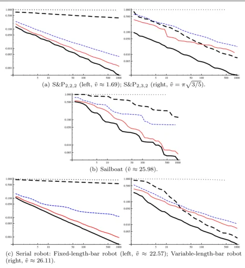
The setting A activates all of the three components we have proposed. The settings B, C and D deactivate one of the three components. The setting E applies the standardBranchAndPrunealgorithm without any modification. Figure 8 illustrates the convergence speeds of the five methods with a log-log scale. A quick look at the graphs shows our method converges much faster for all tested problems. For instance, it took 30 seconds to verify 99% of the workspace of S&P2,2,2 for our

method, compared to 49 and 180 seconds for the settings C and D, settings B and E reaching the timeout with a much lower accuracy (resp. 62% and 5%). As another evidence, after 10 seconds, our method had verified 92% of the volume of the speed diagram of the sailboat problem, against only 80%, 70%, 18% and 0% for the settings C, D, B and E, respectively. In addition, we confirmed that the results computed by our method always converged to the exact volume (or its best known approximation) of these problems.

In Figure 8(b), the graph for our method (setting A) shows sudden speed-ups of the convergence, notably around 5, 20, 80 and 200 seconds, preceded by slow-downs. Following the trace of the solving process, we note the flat portions of the curve correspond to periods of time when almost no new box is verified, hence all boxes are split iteratively until they reach a threshold allowing their verification. Because the search strategy we employ is width-first-search, the boxes in the listL

are then approximately all of the same size and thus, when this threshold is reached for one of them, so it is for the others, which explains the observed speed-ups. The repetition of this behavior is explained by the relative hardness for verifying certain central regions of the speed diagram, which appears clearly in Figure 5(right) paved using a lot of similarly sized boxes. Note that the convergence speed graphs for some computations end before the timeout (1000 seconds) because the solving processes consumed all the memory of the machine (16GB).

We conclude that the combination of the three components is essential in achieving quickly good verified pavings for projection problems. No component appears to be clearly dominated by the others (remark how settings B, C and D compare differently on the different problems) and none seems to have only a negligible influence in general (though setting C, without redundancy pruning by set difference, behaves quite similarly to our method on three problems in our test set, it always remain worse than setting A and behaves much less homogeneously on the whole test set). Another outcome is that, for the well-constrained projec-tion problems, the verificaprojec-tion with box inflaprojec-tion appears the most crucial as the performances without it (settings B and E) are the worst on our test set. Last but not least, this experiment illustrate why standardBranchAndPrunealgorithms

5 10 50 100 500 1000 0.001 0.005 0.010 0.050 0.100 0.500 1.000 5 10 50 100 500 1000 0.005 0.010 0.050 0.100 0.500 1.000

(a) S&P2,2,2 (left, ˜v≈ 1.69); S&P2,3,2(right, ˜v = π

√ 3/5). 5 10 50 100 500 1000 0.005 0.010 0.050 0.100 0.500 1.000 (b) Sailboat (˜v≈ 25.98). 5 10 50 100 500 1000 0.001 0.005 0.010 0.050 0.100 0.500 1.000 5 10 50 100 500 1000 0.005 0.010 0.050 0.100 0.500 1.000

(c) Serial robot: Fixed-length-bar robot (left, ˜v ≈ 22.57); Variable-length-bar robot

(right, ˜v≈ 26.11).

Fig. 8 Comparison of convergence speeds of the methods A–E. The horizontal and vertical

axes represent the time and the proportion of the not-verified volume, respectively.

have been inappropriate to handle projection problems until now, and how it can become drastically better when adapted procedures are used instead.

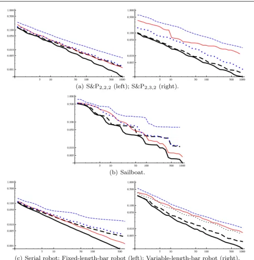
4.2.2 Assessment of the neighborhood management cost

Two of our components, namely the redundancy pruning by set difference and the search strategy with DDRR, require the computation and maintenance of the neighborhood relation between boxes. This is expensive and might be a bottle-neck of the solving process. This evaluation investigates the trade-off between the efficiency of our method and the cost of managing the neighborhood information. Getting rid of neighborhood management requires turning off the two components depending on it. Since we know from the previous experiment that the deacti-vation of one component alone can already be dramatic for the performance of the method, we expect the method without both would be terribly slow. To be

fair, we thus introduce the static dual round-robin strategy (DRR) that fixes the selection ratio of DDRR ass= 1, i.e., oneyvariable is split only when allx vari-ables have been split. DRR does not require the neighborhood information while still incorporating part of the principles of DDRR. We thus compare the following settings:

A. The method with all of the components (thick plain lines). C. The method without the set difference method (thin plain lines).

D. The method without the DDRR strategy, i.e., standard RR is used instead (thin dashed lines).

F. The method using DRR strategy instead of DDRR strategy (dotted lines). G. The method where the set difference method is deactivated, DRR strategy

is activated and the neighborhood management is deactivated (thick dashed lines).

The settings A, C and D are same as in the previous evaluation. The setting F is prepared to evaluate DRR with other components activated. It can be seen as a potential improvement over setting D. The setting G is for the computation without the neighborhood management.

Figure 9 illustrates the convergence speeds of these settings with a log-log scale. The graphs show that the convergence speed of our method (setting A) re-mains always better than the other settings. The computation with the setting C is globally better than the settings F and G for the well-constrained problems. It is interesting to see that, for the under-constrained projection problems, the com-putation without the neighborhood management (setting G) outperforms other settings and achieves the second-best convergence speed.

This experiment consolidates the conclusions from the previous one and desig-nates our method (setting A) with all components activated as the most efficient and robust (as it handles homogeneously well the various problems) among the tested variants.

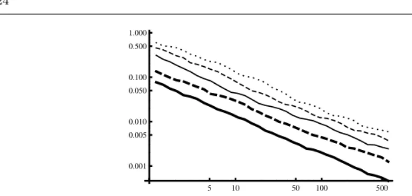
4.2.3 Effect of the Parameter Dimension

In order to evaluate the performance of our method with respect to the size of the problems, we consider a set of instances of the S&Pn,m,p problem in which

the size of the parameter variables is varied. The well-constrained instance scheme S&P2,k,k consists of the constraint (4), wheren= 2, m=k, p=k, and the domain

for the variables is set tox∈[−1,1]2 andy∈[−1,1]k. We solve the instances for

k = 2,3,4,5,6 with our method (setting A from previous experiments). As the

Stopcriterion, we use the timeout check set to 600 seconds.

Figure 10 illustrates the convergence speed of our method with a log-log scale. The lines from bottom to top correspond to harder instances (i.e., bigger values of k), since for a fixed time less inner volume is decided as the line is higher. The exact volume ˜vof each instance isπ√2,π√3/7,π/√3,π√5/17, andπ/2, for

k = 2,3,4,5,6, respectively. We observe that the lines in this figure are almost parallel. In a log-log scale, the slope of the line is related to the degree of the polynomial function that is displayed. Thus parallel lines mean that the complexity of the algorithm is the same for all the instances. This behavior was expected since ideally our method should compute and verify a single box for each projected point. Isolating this box requires a time that grows exponentially with the number

5 10 50 100 500 1000 0.001 0.005 0.010 0.050 0.100 0.500 1.000 5 10 50 100 500 1000 0.005 0.010 0.050 0.100 0.500 1.000

(a) S&P2,2,2(left); S&P2,3,2(right).

5 10 50 100 500 1000 0.005 0.010 0.050 0.100 0.500 1.000 (b) Sailboat. 5 10 50 100 500 0.001 0.005 0.010 0.050 0.100 0.500 1.000 5 10 50 100 500 1000 0.005 0.010 0.050 0.100 0.500 1.000

(c) Serial robot: Fixed-length-bar robot (left); Variable-length-bar robot (right).

Fig. 9 Comparison of convergence speeds of the methods A, C, D, F and G.

of projected variables (as for any bisection algorithm), but the convergence speed of the algorithm should remain proportional whatever this dimension, i.e., the proportion of the verified projection should grow as fast with the time for any number of projected variables. This is observed in this experiment, giving high hopes our method could deal with larger scale projection problems.

5 Conclusion

We have presented a numerical algorithm that can compute an inner and an outer approximation of the projection of the solution set to an under-constrained prob-lem. The proposed algorithm is a simple adaptation of the standardBranchAndPrune

algorithm for NCSPs. The modifications are designed as separate procedures, namely those for verification, pruning, branching strategies, and they embed heuris-tics for optimizing the performance of the algorithm.

5 10 50 100 500 0.001 0.005 0.010 0.050 0.100 0.500 1.000

Fig. 10 Comparison of the volume computation of the S&P2,k,k problem (k = 2, 3, 4, 5, 6).

Our method is more generic than the existing interval methods in the sense that we consider systems described by an arbitrary number of variables and constraints, which can be inequality constraints. It is also more general in the sense it can make use of all the techniques available to handle efficiently constraints in the

BranchAndPrune algorithm, e.g., all pruning operators are applicable. Finally, it

can be adapted in order to handle under-constrained projection problems. Many problems in control and robotics can be directly encoded as under-constrained NCSPs, and a paving of a projected solution set provides a mean for analyzing the problem. In the experiments, we have shown the applicability of our method to problems of interest in control and robotics.

The experimental results demonstrate the quality of the output of the proposed method and its efficiency with respect to prior methods, including ones much more specifically designed for the projection problem and limited in scope.

Acknowledgements This work was partially funded by the ANR grant number PSIROB06

174445 and the JSPS grant KAKENHI 23-3810. The machine used for the experiments was supported by Prof. Kazunori Ueda.

References

1. Araya, I., Trombettoni, G., Neveu, B.: Exploiting monotonicity in interval constraint prop-agation. In: Proc. of AAAI’10 (2010)

2. Beltran, M., Castillo, G., Kreinovich, V.: Algorithms that still produce a solution (maybe not optimal) even when interrupted: Shary’s idea justified. Reliable Computing 4(1), 39–53 (1998)

3. Benhamou, F., McAllester, D., Van Hentenryck, P.: CLP(Intervals) revisited. In: Proc. of Intl. Symp. on Logic Prog., pp. 124–138. The MIT Press (1994)

4. Collins, G.E.: Quantifier elimination by cylindrical algebraic decomposition – twenty years of progress. Quantifier Elimination and Cylindrical Algebraic Decomposition pp. 8–23 (1998)

5. Goldsztejn, A.: A Branch and Prune Algorithm for the Approximation of Non-Linear AE-Solution Sets. In: Proc. of ACM SAC 2006, pp. 1650–1654 (2006)

6. Goldsztejn, A., Jaulin, L.: Inner and outer approximations of existentially quantified equal-ity constraints. In: Proc. of CP’06, LNCS 4204, pp. 198–212 (2006)

7. Goldsztejn, A., Jaulin, L.: Inner approximation of the range of vector-valued functions. Reliable Computing 14, 1–23 (2010)

8. Goualard, F.: Gaol: NOT Just Another Interval Library (version 3.1.1). http://sourceforge.net/projects/gaol/ (2008)

9. Granvilliers, L.: Realpaver (version 1.1). http://pagesperso.lina.univ-nantes.fr/ granvilliers-l/realpaver/ (2010)

10. Hansen, E., Sengupta, S.: Bounding solutions of systems of equations using interval anal-ysis. BIT 21, 203–211 (1981)

11. Herrero, P., Jaulin, L., Vehi, J., Sainz, M.: Guaranteed set-point computation with ap-plication to the control of a sailboat. International journal of control, automation and systems 8(1), 1–7 (2010)

12. Herrero, P., Sainz, M.A., Veh, J., Jaulin, L.: Quantified set inversion algorithm with ap-plications to control. Reliable Computing 11(5), 369–382 (2005). DOI 10.1007/s11155-005-0044-1

13. Jaulin, L., Kieffer, M., Didrit, O., Walter, E.: Applied Interval Analysis, with Examples in Parameter and State Estimation, Robust Control and Robotics. Springer-Verlag, London (2001)

14. Kearfott, R.B., Nakao, M.T., Neumaier, A., Rump, S.M., Shary, S.P., Van Hentenryck, P.: Standardized notation in interval analysis. In: Proc. of XIII Baikal International School-seminar “Optimization methods and their applications”, pp. 106–113 (2005)

15. Kearfott, R.B., Novoa III, M.: Algorithm 681: Intbis, a portable interval newton/bisection package. ACM Trans. on Math. Softw. 16(2), 152–157 (1990)

16. Khalil, H.K.: Nonlinear Systems, Third Edition. Prentice Hall (2002)

17. Lhomme, O.: Consistency techniques for numeric CSPs. In: Proc. of the 13th International Joint Conference on Artificial Intelligence (IJCAI’93), pp. 232–238 (1993)

18. Moore, R.: Interval Analysis. Prentice-Hall (1966)

19. Neumaier, A.: The enclosure of solutions of parameter-dependent systems of equations. In: R. Moore (ed.) Reliability in Computing, pp. 269–286. Academic Press, San Diego (1988) 20. Neumaier, A.: Interval Methods for Systems of Equations. Cambridge University Press

(1990)

21. Ratschan, S.: Uncertainty propagation in heterogeneous algebras for approximate quanti-fied constraint solving. Journal of Universal Computer Science 6(9), 861–880 (2000) 22. Reboulet, C.: Mod´elisation des robots parall`eles. In: J.D. Boissonat, B. Faverjon, J.P.

Merlet (eds.) Techniques de la robotique, architecture et commande, pp. 257–284. Hermes sciences, Paris, France (1988)

23. Rossi, F., van Beek, P., Walsh, T.: Handbook of Constraint Programming (Foundations of Artificial Intelligence). Elsevier Science Inc., New York, NY, USA (2006)

24. Shary, S.P.: A new technique in systems analysis under interval uncertainty and ambiguity. Reliable Computing 8(5), 321–418 (2002)

25. Van Hentenryck, P., Michel, L., Deville, Y.: Numerica : A Modeling Language for Global Optimization. MIT Press (1997)