HAL Id: hal-01410191
https://hal-mines-paristech.archives-ouvertes.fr/hal-01410191
Submitted on 6 Dec 2016
HAL is a multi-disciplinary open access
archive for the deposit and dissemination of
sci-entific research documents, whether they are
pub-lished or not. The documents may come from
teaching and research institutions in France or
abroad, or from public or private research centers.
L’archive ouverte pluridisciplinaire HAL, est
destinée au dépôt et à la diffusion de documents
scientifiques de niveau recherche, publiés ou non,
émanant des établissements d’enseignement et de
recherche français ou étrangers, des laboratoires
publics ou privés.
Serge Antoine Séguret, Sebastian de la Fuente
To cite this version:
Serge Antoine Séguret, Sebastian de la Fuente. Drill-Holes and Blast-Holes. Geostat 2016, Sep 2016,
valencia, Spain. �hal-01410191�
Serge Antoine Séguret1 and Sebastian De La Fuente2
AbstractThe following is a geostatistical study of copper measurements on sam-ples from diamond drill-holes and blast-holes.
Both measurements are formally compared, leading to a model where a blast-hole can be considered a regularization of the drill information up to a nugget effect characteristic of the blast-holes.
This formal link makes it possible to build a cokriging system that takes into ac-count the different supports and leads to a block model based on blast and drill-holes.
The model is tested on a realistic simulation where the true block grades, which are known, are compared to their estimate obtained by:
- Kriging using only drill-holes; - Kriging using only blast-holes;
- Cokriging using drill and blast-holes together.
A preliminary conclusion is that the best estimates are obtained when only blasts or alternatively, blast and drill-holes are used; there is no significant difference be-tween the two, which is due to the great amount of blast information. This result justifies the usual practice of basing short-term planning on blasts only. But an-other conclusion may be drawn when kriging is compared to a moving average (another common practice), both based on blasts: depending on the number of data used in the neighborhood, the moving average produces a strong conditional bias. As a byproduct, we also show how it is possible to filter the blast error by kriging and to make a deconvolution to estimate point support values using blast meas-urements.
Introduction
Typically, in open-pit mines, geologists, mining engineers, metallurgists, have at their disposal two types of grade measurements: those from drill-holes and those from blast-holes. Because they are much more expensive, the drill-holes (diamond ones in our case) are fewer than the blast-holes and sampling rates ranging from one over three to one over ten or worse are frequent. Another difference concerns the way the measurements are used. Drill-holes are used for medium- and long-term planning; blast-holes for short-long-term planning without any need for
geostatistics; a simple moving average is often used to estimate the block quantity of the metal. The use of two types of measurements, that are supposed to represent the same thing, raises questions about their relationship. In particular, would it not
1 Mines ParisTech, PSL Research University, Geosciences Center, Geostatistical Team, 35 rue Saint Honoré, 77300, Fontainebleau, France, [email protected] 2 Codelco, Radomiro Tomic, Chile, [email protected]
be possible to enrich the short-term estimates, now based only on blast-holes, by adding the drill-holes measurement as they arrive? Another question, is it permit-ted to use a simple moving average based on blast-holes for the block estimation? Finally, it is often said, without real justification, that the diamond drill-holes are much better than the blast ones. We ask: better in what way, better for what, and is it true?
After having modeled this relationship, we present some linear systems that make it possible to filter the nugget effect of the blast-holes, removing their regulariza-tion effect and using the blast and the drill-holes together in a single linear system. These are just demonstrative exercises; one can imagine other possibilities result-ing from the formal link between two types of measurements known over two dif-ferent supports.
Formal link
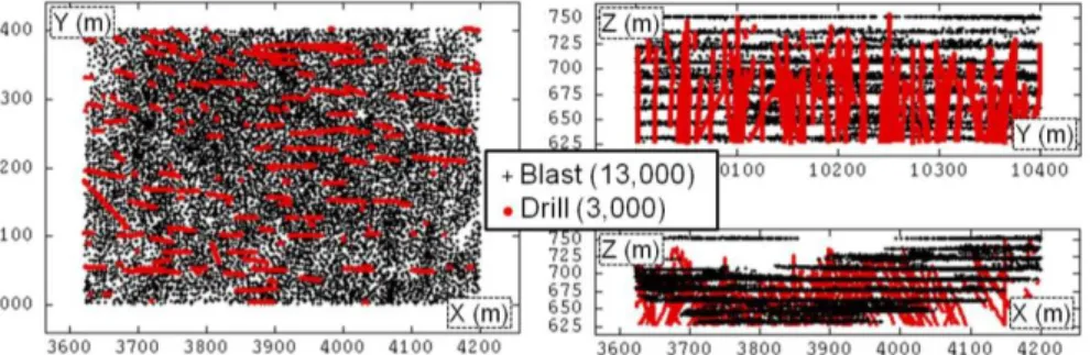
The initial data (Figure 1) are from an open-pit copper mine in Northern Chile where a subdomain was chosen for analysis because it is almost homogeneously covered by around 3,000 drill-hole samples (3m long) and 13,000 blast-hole sam-ples (15m long). In this case study, the diameters of the drill-holes and blast-holes are considered to be the same.
Figure 1. Base maps of blast (black) and drill (red) measurements
In a previous paper (Séguret, 2015), the author showed that if we omit the problem of the nugget effect, both blast- and drill-holes can be considered a regularization of the same phenomenon in accordance with their respective supports. But the drill-holes have their own errors, independent of the blast ones, so that they do not share the nugget effect and finally, we have:
15
( , , ) ( , , ) ( ) ( , , )
blast m
Y x y z Y x y z p z R x y z (1)
with
Y(x,y,z), the point grade assumed to be isotropic and without any meas-urement error;
“*” denotes a convolution product;
15 15 ( , , ) m( ) ( , , ) m( ) Y x y z p z Y x y u p z u du
;15 15 [0, ] 2 1 ( ) 1 (| |) 15 m
p z z , the convolution function;
15 [0, ]
2
1 (| |)z the indicator function equal to 0 outside the interval [-7.5m,
7.5m] and 1 inside it;
R(x,y,z), a “white noise” residual, statistically and spatially independent of Y(x,y,z) and representing the blast error
The variogram of Yblast(x,y,z) becomes:
15 ( ) ( ) ( ) blast h m h R h (2) with ( ) R h
, the nugget effect due to the blast error, with the variance 2
R
;
15m( )h P15m ( )h P15m (0)
, regularized variogram expressed as a convolution product;
, the point variogram, assumed to be isotropic;
15 15 15 2 [0,15] 1 ( ) ( ) ( | | 15)1 (| |) 15 m m m P h p p h h h , function with “P”(upper case) that regularizes the variogram, expressed as an auto-convolution product of p15m (lower case) as previously defined by itself. Similar equations can be established for the drill-holes and the 3 m support. The model assumes that the blast and the drill samples have the same average because the independent residuals are of zero mean.
Resulting linear systems
From equations (1) and (2) some linear systems can be deduced, in the following we propose three of them that are tested on a conditional simulation.
1 Removing the blast error by kriging
One can remove the blast error by “Factorial Kriging” estimation (Matheron, 1982), using a linear system applicable to each blast measurement and a local neighborhood of surrounding blast samples. The system is presented symbolically by matrix formalism:
(I)
In this system, Rdisappears from the second member of the linear system and is
replaced by 2R, the value of the nugget effect. Thus, we remove, from the estima-tion, the part associated with the measurement error. This does not mean that there is no nugget effect in the remaining part 15m; it means that only the “natural” part remains. In our case, the complete nugget effect has to be removed because blasts
and drills do not share any micro-structure.
The result of the estimation is the average value of the grade over the blast support at blast-sample locations with no measurement error.
2 Deconvolution by kriging
It may be interesting to remove the effect on the blast of regularization by using a kriging system which estimates, for each blast measurement, a “point” value while simultaneously removing the part of the nugget effect associated with blast errors:
(II)
The difference with the previous system is that in the second member, 15m P15m ( P15m)(0)
(upper case P) is replaced by( p15m) ( p15m)(0)
(lower case p). Initially developed to improve microscopy images of thin plates in the petroleum industry (Séguret,1988; Le Loch, 1990), deconvolution by kriging was later compared to other approaches (Jeulin, 1992) and has sometimes been used in recent years, for example by Desnoyers, 2014.
3 Block estimate by cokriging drill- and blast-measurements
Finally, one can imagine renewing the mine planning block model locally by us-ing blast and drill samples together in a cokrigus-ing system with a linked mean (same average for both measurements, Chiles, 2012):
As usual, the matrix on the left in the linear system concerns only the data; here, a set of drill and blast measurements. As a consequence, it is composed on the diagonal of sub matrices where the variogram of the drill-holes (regularization over 3m) and the variogram of the blast-holes (regularization over 15m) appear. The cross sub matrix, which concerns the link between blast- and drill-holes, is based on a regularization of the point support variogram over both supports, which is the reason why 3 ,15m m p3mp15m ( p3mp15m)(0)intervenes. Compared
to a usual cokriging system that one can find in the literature (Wackernagel, 2003), the linked mean constraints reduce to one line and one column the sub matrix associated with the non-bias constraints. Without this simplification, there would be two lines and two columns. In practice, the consequence is important because here the drill and blast measurements play the same role while in a normal cokriging system, one of the measurement types would be considered auxiliary, thus reducing its relative influence on the final result. In the right-hand vector, the term pVappears because the objective is to estimate the average grade over a v-sized block. This convolution is combined with previous regularizations.
Simulation
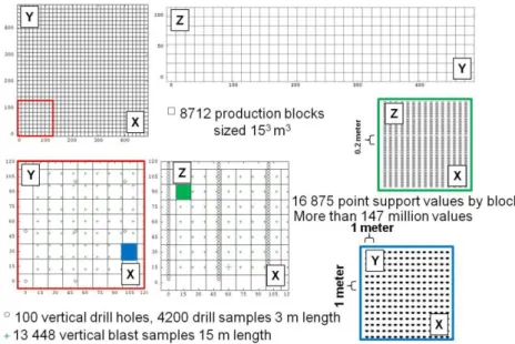
A refined simulation of point-support grades was made every meter horizontally and every 20 cm vertically. It reproduces the data-set properties. Then, 100 verti-cal drill-holes were created by averaging, every 50 m horizontally, all the values along 3 m vertically. In this way we obtained 4,200 drill samples. Similarly, more than 13,000 vertical 15 m-long blast-holes were produced with a horizontal spac-ing of 12 m. The true 153 m3 block value is found by averaging more than 16,000 point-support values contained in the block. The sampling ratio is approximately one drill-hole sample to three blast-hole samples and the domain covered by the simulation is 500 by 500 m2 horizontally and 125 m vertically. The following fig-ure summarizes the grids involved.
Figure 2. Blast- and drill-holes grid nodes involved in the simulation
For simplification, the drill samples have no errors. We add to the blast samples a random noise with a nugget effect of 0.02, representing the blast sampling error. The grades are realistic with a 0 minimum, 3.5 % maximum; an average of 0.63 % as in the real deposit and the distribution is correctly skewed to the right. We veri-fy that the sills of the drill, blast and block variograms obey the laws of regulariza-tion by following the procedure presented in Séguret (2015) which is based on the charts by Journel (2003) pages 125-147. Figure 3 shows the result.
Figure 3. From left to right, properties of point-support simulated grades, 3m support, 15m and blocks. Upper figures are experimental histograms, bottom variograms.
Removing the blast error by kriging
In the first test we propose to remove the blast error by using the linear system (I). This filter can be applied to every blast measurement, using a local neighborhood of surrounding blast samples. The neighborhood must contain the sample from which the noise is to be removed; otherwise, the filtering is not efficient. For comparison, the estimation is made by kriging with no filtering, using the same neighborhood (but without the target sample, otherwise the kriging will ob-viously give back the value of the data point).
We select, among all the simulated blasts, a subset of around 1,000 samples on which estimations will be conducted, using the additional samples in case of ordi-nary kriging and all the samples in case of nugget filtering.
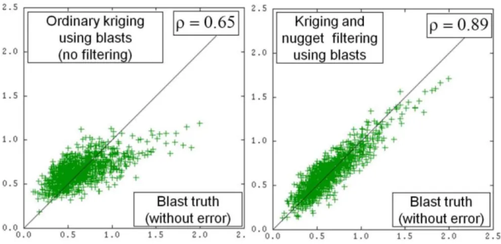
The reference is the “truth” i.e. the blast without errors which we know because we work on a simulation where everything is known. Figure 4 shows the results.
Figure 4. Scatter diagrams between the true values (horizontal axis) and estimations (verti-cal axis). Left figure, ordinary kriging estimation; right figure, estimation where the blast error is removed by kriging.
On these scatter diagrams the horizontal axis represents the true blast value with-out any sampling error. On the left-hand scatter diagram, the vertical axis is a usu-al kriging. The correlation with the truth is 0.65. On the right-hand one, when the filtering is activated, the correlation increases to 0.896. Why?
With filtering, the kriging neighborhood can incorporate the target point where the filter is applied. This point takes a high kriging weight (more than 65%). Although noisy, this point is closer to the truth than any average based on surrounding points which explains why the filter estimate is closer to the truth.
Finally, the advantage of this linear system (I) is to enable the kriging neighbor-hood to incorporate the target point information.
Deconvolution by kriging
Now we propose a second test: removing the effect of regularization on the blast with a kriging system that estimates a “point” value for each blast measurement, while simultaneously removing the part of the nugget effect associated with blast errors. By this procedure, we expect to restore the initial variability of the point-support value judged to be too strongly smoothed by the regularization. The linear system used is (II).
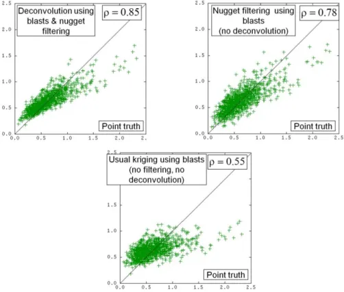
A comparison is made with the true point value and with previous estimates (esti-mating a blast with or without nugget effect). Figure 5 shows the results.
Figure 5. Scatter diagrams between the true values (horizontal axis) and estimations (verti-cal axis). Upper left figure, deconvolution together with error filtering; upper right figure, error removal without deconvolution; bottom figure, no deconvolution, no error filtering.
In the three scatter diagrams, the horizontal axis represents the true point-support value. The upper left-hand scatter figure presents the result when a deconvolution is made jointly with error filtering. The correlation with the true value is good at 0.85.
The upper right-hand figure presents the result of the error removal with no deconvolution. It corresponds to the previously presented system but this time as
compared with the point-support value; this is the reason why the correlation is 0.78 and not 0.89 when compared to the blast values. In comparison with the left-hand figure, the deconvolution increases significantly the accuracy of the estima-tion.
The bottom figure shows the results when neither filtering nor deconvolution is done. The correlation is very low, it is 0.55.
As for nugget filtering, the deconvolution is efficient because the linear system
au-thorizes the use of the target points where the filter is applied.
Block estimate by cokriging of drill and blast measurements
The third test is made to renew the mine planning block model locally by using blast and drill samples together. The system used is (III), a cokriging system with linked mean because drill and blast samples have the same average, which is man-datory for carrying out all these calculations.
Our objective is to estimate the average grade at the block scale and we compare it with two other systems: block grade estimate by kriging using only drill-holes and block grade estimate by kriging using only blast-holes. Figure 6 shows the results.
Figure 6. Scatter diagrams between the true values (horizontal axis) and estimations (verti-cal axis). Upper left figure, estimation is kriging using drill-holes; upper right figure, kriging using blast-holes; bottom figure, kriging using both blast and drill samples together.
For the three previous scatter diagrams, the horizontal axis is the true block grade. The upper left-hand diagram is the result obtained by ordinary kriging with drill samples; the upper right-hand diagram is the result obtained with blast samples. The jump by the correlation coefficient from 0.38 (OK using drills) to 0.88 (OK using blasts) is impressive. Even if the blast samples are regularized over 15m, the fact that they are more numerous and respect the variogram (up to a nugget effect) justifies their use when possible, in selections for mining operations, instead of the drill samples.
The bottom diagram concerns cokriging using blast and drill samples together. The performance is similar to ordinary kriging with blast samples only. In our case cokriging is not useful because the blasts are so numerous that adding a drill con-tribution does not improve the results. This does not mean that such a system is not helpful, for example in short-term planning to evaluate a domain to be blasted where there are only drill-holes.
Moving average or kriging?
In our case, short-term planning is based on averages using the blast samples in-cluded in the block, so the question is whether kriging can produce an improve-ment. We are comparing three experiments:
• Ordinary kriging with 24 surrounding blast measurements (previous work);
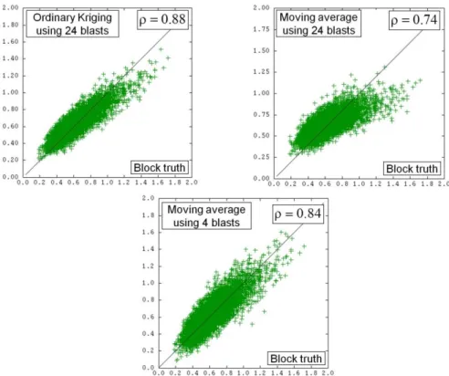
• Moving average with the same 24 surrounding blast measurements; • Moving average with 4 blast measurements at the same elevation. Figure 7 shows the results.
Figure 7. Scatter diagrams between the true values (horizontal axis) and estimations (verti-cal axis). Upper left, ordinary kriging with 24 surrounding blast measurements; upper right, moving average with the same 24 surrounding blast measurements; bottom, moving average with 4 blast measurements of the same elevation.
Replacing ordinary kriging by an average reduces the correlation with the truth from 0.88 to 0.74. This is a very large reduction which should encourage the prac-titioners to use kriging instead of present practices in the company.
If practitioners do not want to change their habits, one can see that with only four points, the result is better than when 24 points are used because the smoothing is weaker: the correlation with the truth increases from 0.74 to 0.84, a result still be-low the one obtained with kriging but very close to it. Does this mean that we rec-ommend a moving average with only 4 points? NO! To use so few points is risky for reasons of conditional bias. To illustrate this concept, consider again the previ-ous scatter diagram but this time, with the true block grade for the vertical axis and the estimate on the horizontal axis (figure 8).
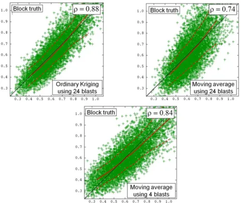
Figure 8. Scatter diagrams between the true values (vertical axis) and estimations (horizon-tal axis). Upper left: the horizon(horizon-tal axis represents ordinary kriging with 24 surrounding blast measurements (previous work); upper right: the horizontal axis represents a moving average with the same 24 surrounding blast measurements; bottom: the horizontal axis rep-resents a moving average with 4 blast measurements at the same elevation.
In the previous figures, red continuous curves represent the mathematical expec-tations of the true values conditioned by different estimates. We focus on the most representative [0.3%, 1%] range of grades.
When kriging is done with 24 points, the conditional expectation curve is close to the first diagonal. Thus, when we select the block according to its estimation, we obtain, on average, what we expect, with perhaps a slight tendency to underesti-mate the high grades
When we replace kriging by a moving average using 24 points, the red curve is still close to the diagonal, with a slight tendency to overestimate the low grades and underestimate the high ones
When the moving average is done with only 4 points, the conditional bias appears clearly: in the range of the low grades, we systematically underestimate the aver-age grade of the blocks and may decide to classify as “waste” blocks that are in reality richer than expected. Conversely, in the range of the high grades, this
mov-ing average with only 4 points systematically overestimates the average grade of the block so that we classify as “rich” blocks which must be considered “waste”. It is for this reason that one must use enough points in the kriging neighborhood for grade control, and reflect on the reason why kriging and geostatistics were cre-ated (Matheron, 1971).
Conclusion
The study of a porphyry copper deposit showed a formal link between blast- and drill-holes, leading to numerous linear systems able at least, to filter blast errors, make blast deconvolution or build a block model using blasts and drills together; techniques that could be used at different stages of the mining process.
Tested on a realistic simulation, these systems have proved their worth, as well as the danger of replacing kriging by a moving average, especially with few points, producing a strong conditional bias, and this is a useful reminder of the reason why kriging was created.
Overall, a formal comparison between blast- and drill-holes shows that in this mine – and more generally, in this company – the quality of the blast values is as good as the quality of the drill values, contrary to conventional wisdom.
Bibliography
Séguret, S. A., (2015) Geostatistical comparison between blast and drill-holes in a porphyry copper deposit. WCSB7 7th world conference on sampling and blending, Jun 2015, Bordeaux, France. 2015, DOI : 10.1255/t0sf.51. Matheron, G., (1971). The theory of regionalized variables and its applications.
Fasc. 5, Paris School of Mines, Fontainebleau, France.
Matheron, G., 1982. Pour une Analyse Krigeante des données Régionalisées. Mines ParisTech publication N-732. Center for Geostatistics, Fontaine-bleau, France.
Séguret, S.A., (1988). Pour une méthodologie de déconvolution de variogrammes. Mines ParisTech publication N-51/88/G. Center for Geostatistics, Fon-tainebleau, France.
Le Loch, G.(1990) Déconvolution d’images scanner. Mines ParisTech publication N-8/90/G. Center for Geostatistics, Fontainebleau, France
Jeulin, D., Renard, D., (1992). Practical limits of the deconvolution of images by kriging. Microsc., Microanal., Microstruct., Volume 3, Number 4, DOI: 10.1051/mmm:0199200304033300.
Desnoyers, Y., Dogny, S., (2014). Geostatistical deconvolution with non destruc-tive measurements for radiological characterization of contaminated fa-cilities in 10th GEOENV conference, in Presse des Mines, Paris, DOI
9782356711366.
Chilès, J. P., Delfiner, P., (2012). Modeling Spatial Uncertainty, Wiley edition. Wackernagel, H. (2003). Multivariate geostatistics, Springer sciences. Journel, A.,G., Huijbregts, Ch., J., (2003). Mining Geostatistics, the Blackburn