HAL Id: hal-00931844
https://hal.inria.fr/hal-00931844
Submitted on 15 Jan 2014
HAL is a multi-disciplinary open access
archive for the deposit and dissemination of
sci-entific research documents, whether they are
pub-lished or not. The documents may come from
teaching and research institutions in France or
abroad, or from public or private research centers.
L’archive ouverte pluridisciplinaire HAL, est
destinée au dépôt et à la diffusion de documents
scientifiques de niveau recherche, publiés ou non,
émanant des établissements d’enseignement et de
recherche français ou étrangers, des laboratoires
publics ou privés.
Factored Planning: From Automata to Petri Nets
Loïg Jezequel, Eric Fabre, Victor Khomenko
To cite this version:
Loïg Jezequel, Eric Fabre, Victor Khomenko. Factored Planning: From Automata to Petri Nets.
In-ternational Conference on Application of Concurrency to System Design (ACSD), Jul 2013, Barcelone,
Spain. �hal-00931844�
Factored Planning: From Automata to Petri Nets
Lo¨ıg Jezequel ENS Cachan Bretagne
IRISA Rennes, France [email protected]
Eric Fabre
INRIA Rennes Bretagne Atlantique IRISA
Rennes, France [email protected]
Victor Khomenko School of Computing Science
Newcastle University Newcastle, United Kingdom
Abstract—Factored planning mitigates the state space explo-sion problem by avoiding the construction of the state space of the whole system and instead working with the system’s components. Traditionally, finite automata have been used to represent the components, with the overall system being represented as their product. In this paper we change the representation of compo-nents to safe Petri nets. This allows one to use cheap structural operations like transition contractions to reduce the size of the Petri net, before its state space is generated, which often leads to substantial savings compared with automata. The proposed approach has been implemented and proven efficient on several factored planning benchmarks.
I. INTRODUCTION
Planning consists in organising a set of actions in order to reach some predefined (set of) goal state(s), where each action modifies some of the state variables of the considered system. In that sense, planning is very similar to reachability analysis in model checking, or to path search in a graph, viz. the state graph of the system. A solution to these problems is either an action plan reaching the goal, or an example of a run proving the reachability, or a successful path in a graph. These problems have much benefited from the introduction of true concurrency semantics to describe plans or runs [1]. Con-currency represents the possibility to execute simultaneously several actions that involve different subsets of resources. With such semantics, a plan or a trajectory becomes a partial order of actions rather than a sequence, which can drastically reduce the number of trajectories to explore.
In the planning community, it was soon observed that concurrency could be turned into an ally, as one can avoid the exploration of meaningless interleavings of actions. The first attempt in that direction was Graphplan [2], which lays plans on a data structure representing explicitly the parallelism of actions. This data structure has connections with merged processes [3] and trellis processes [4], where the conflict rela-tion is non binary and can not be checked locally. Graphplan did not notice specifically these facts, and chose to connect actions with a loose and local check of the conflicts. Hence the validity of the extracted plans had to be checked, and numerous backtrackings were necessary. A more rigourous approach to concurrent planning was later proposed by [5] and improved in [6]. The idea was to represent a planning problem as an accessibility problem for a safe Petri net (possibly with read arcs). One can then represent concurrent runs of the net
using unfoldings, and the famous A* search algorithm was adapted to Petri net unfoldings.
An alternative and indirect way to take advantage of concur-rency in planning problems is the so-called factored planning approach. It was first proposed in [7], and variations on this idea were described in [8], [9]. Factored planning consists in splitting a planning problem into simpler subproblems, involving smaller sets of state variables. If these subproblems are loosely coupled, they can be solved almost independently, provided one properly manages the actions that involve several subproblems. In [9], the problem was expressed under the form of a network (actually a product) of automata, that must be driven optimally to a target state. A plan in this setting is a tuple of sequences of actions, one sequence per component, these sequences being partly synchronised on some shared events. In this representation, a plan is again a partial order of actions, and the concurrency between components is maxi-mally exploited. This is what we call the global concurrency, the concurrency of actions living in different components. However, this approach fails to take advantage of a local concurrency, that would be internal to each component or each subproblem. This is specifically the point addressed by this paper: we replace the automaton encoding a planning sub-problem (which we call a component) by a Petri net, in order to represent internal concurrency of this component. We therefore encode a planning problem as a product of Petri nets, and explore the extension of our distributed planning techniques to this setting.
The contributions of this paper can be summarised in the following points.
First, it reconciles local and global concurrency in the factored planning approach. This means taking advantage both of the concurrency between components of a large planning problem, or equivalently of the loose coupling of planning subproblems, and of the concurrency that is internal to each component. In other words, this paper demonstrates that the planning approach proposed in [5] can be coupled with dis-tributed/factored planning ideas as developed in [9]. The main move consists in replacing modular calculations performed on automata by calculations performed on Petri nets.
Secondly, these ideas are experimentally evaluated on stan-dard benchmarks from [10], in order to demonstrate the gains obtained by exploiting the local concurrency within each component. In particular, we compare the runtimes of the
distributed computations described in [9] with those obtained when automata are replaced by Petri nets.
Finally, we show to which extent the results of [11] on the projection of Petri nets can be extended to the case of Petri nets with costs on transitions. This permits cost-optimal planning.
II. PETRI NETS AND FACTORED PLANNING
This section recalls the standard STRIPS propositional for-malism that is commonly used to describe planning problems. It then explains how factored planning problems can be recast into an accessibility problem (or more precisely a fireability problem for a specific labelled transition) for a product of Petri nets.
A. Planning problems
A planning problem is a tuple (A, O, i, G) where A is a set of atoms, O ⊆ 2A× 2A× 2A is a set of operators or
actions. A state of the planning problem is an element of 2A, or equivalently a subset of atoms. i ⊆ A is the initial state, and G ⊆ A defines a set of goal states as follows: s ⊆ A is a goal state iff G ⊆ s. An operator o ∈ O is defined as a triple o = (pre, del, add) where pre is called the precondition of o, del is called its negative effect, and add is called its positive effect. The operator o = (pre, del, add) is enabled from a state s ⊆ A as soon as pre ⊆ s. In this case o can fire, which leads to the new state o(s) = (s \ del) ∪ add. The objective of a planning problem is to find a sequence p = o1. . . on of operators such
that i enables o1, for any k ∈ [2..n], ok−1(. . . (o1(i))) enables
ok, and on(. . . (o1(i))) ⊇ G.
One can directly translate a planning problem into a directed graph, where the nodes of the graph represent the states and the arcs are derived from the operators. Solutions to the planning problem are then paths leading from i to goal states. Tradi-tional planners thus take the form of path search algorithms in graphs: most of them derive from the well-known A* algorithm [12] and provide plans as sequences of operator firings. A more recent set of works tried to take advantage of the locality of operators: they involve limited sets of atoms, which means that some operators can fire concurrently. This leads to the idea of providing plans as partial orders of operator firings rather than sequences. These approaches rely on the translation of planning problems into safe Petri nets [5], and look for plans using unfolding techniques [13] in combination with an adapted version of A* [6].
B. Petri nets and planning problems
A net is a tuple (P, T, F ) where P is a set of places, T is a set of transitions, P ∩ T = ∅, and F : (P × T ) ∪ (T × P ) → N is a flow function. For any node x ∈ P ∪ T , we denote by
•x the set {y : F ((y, x)) > 0} of predecessors of x, and
by x• the set {y : F ((x, y)) > 0} of successors of x. In a net, a marking is a function M : P → N associating an natural number to each place. A marking M enables a transition t ∈ T if ∀p ∈ •t, M (p) ≥ F ((p, t)). In such a case, the firing of t from M leads to the new marking Mt
such that ∀p ∈ P, Mt(p) = M (p) − F ((p, t)) + F ((t, p)). In
the sequential semantics, an execution from marking M is a sequence of transitions t1. . . tn such that M enables t1, and
for any k ∈ [2..n], Mt1...tk−1 enables tk (where Mt1...ti is defined recursively as Mt1...ti = (Mt1...ti−1)ti). We denote by hM i the set of executions from a marking M .
A Petri net is a tuple (P, T, F, M0) where (P, T, F ) is a net and M0 is the initial marking. In a Petri net, a marking
M is said to be reachable if there exists an execution t1. . . tn
from M0 such that M = M0
t1...tn. A Petri net is said to be k-bounded if any reachable marking M is such that ∀p ∈ P, M (p) ≤ k. It is said to be safe if it is 1-bounded.
A labelled Petri net is a tuple (P, T, F, M0, Λ, λ) where
(P, T, F, M0) is a Petri net, Λ is an alphabet, and λ : T →
Λ ∪ {ε} is a labelling function associating a label from Λ ∪ {ε} to each transition. The special label ε is never an element of Λ and the transitions with label ε are called silent transitions. In such a labelled Petri net, the word associated to an execution o = t1. . . tn is λ(o) = (λ(t1) . . . λ(tn))|Λ(so
silent transitions are ignored). The language of a labelled Petri net N = (P, T, F, M0, Λ, λ) is the set L(N ) of all the words corresponding to executions from M0 in N :
L(N ) = {λ(o) : o ∈ hM0i}.
[5] proposed the representation of planning problems as safe labelled Petri nets. Each atom was represented by a place, and for technical reasons – namely to guarantee the safeness of the Petri net – [5] also introduced complementary places representing the negation of each atom. The initial state i naturally gives rise to the initial marking M0. An operator o is then instantiated as several transitions labelled by o, one per possible enabling of this operator. This duplication is due to the fact that an operator can delete of an atom that it does not request as an input, and thus that could either be present or not. The goal states, corresponding to goal markings of the Petri net, are then captured using an additional transition that consumes the tokens in the places representing the atoms G, which is thus enabled iff a marking corresponding to some goal state has been reached.
From now on we consider that a planning problem is a pair ((P, T, F, M0, Λ, λ), g) where (P, T, F, M0, Λ, λ) is a safe labelled Petri net and g ∈ Λ is a particular goal label. In such a problem one wants to find an execution o = t1. . . tn
from M0 such that for any k ∈ [1..n − 1], λ(tk) 6= g and
λ(tn) = g.
C. Petri nets and factored planning problems
A factored planning problem is defined by a set of inter-acting planning sub-problems [7], [8], [9]. These interactions can take the form of shared atoms or of shared actions, but one can simply turn one model into its dual. So we choose here the synchronisation on shared actions, which naturally fits with the notion of synchronous product. In the context of Petri nets, a factored planning problem takes the form of a set of Petri nets synchronised on shared transition labels: if two nets share a transition label σ, the transitions of these nets labelled by σ have to be fired simultaneously. This synchronisation on
shared labels – which corresponds to the synchronisation on shared actions for planning problems – can be formalised as the product of labelled Petri nets.
The product of two labelled Petri nets N1 and N2 (with
alphabets Λ1 and Λ2) is a labelled Petri net N = N1× N2
(with alphabet Λ1∪ Λ2) representing the parallel executions
of N1 and N2 with synchronisations on common transition
labels from Λ1∩ Λ2 (notice that ε is never a common label
as, by definition, it never belongs to Λ1nor Λ2). It is obtained
from the disjoint union of N1 and N2 by fusing each
σ-labelled transition of N1 with each σ-labelled transition of
N2, for each common action σ, and then deleting the original
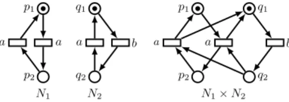
transitions that participated in such fusions. An example is given in Figure 1. N1 p1 a p2 a N2 q1 a q2 b N1× N2 p1 a p2 q1 q2 b a
Fig. 1: Two Petri nets and their product
Formally, if N1 = (P1, T1, F1, M10, Λ1, λ1) and N2 =
(P2, T2, F2, M20, Λ2, λ2), then N = (P, T, F, M0, Λ, λ) with:
P = P1 ∪ P2, T = {(t1, t2) : t1 ∈ T1, t2 ∈
T2, λ1(t1) = λ2(t2) 6= ε} ∪ {(t1, ?) : t1 ∈ T1, λ1(t1) /∈
Λ2} ∪ {(?, t2) : t2 ∈ T2, λ2(t2) /∈ Λ1}, F ((p, (t1, t2)))
equals F1((p, t1)) if p ∈ P1 and else equals F2((p, t2)),
F (((t1, t2), p)) equals F1((t1, p)) if p ∈ P1 and else equals
F2((t2, p)), M0(p) equals M10(p) for p ∈ P1 and else equals
M0
2(p), Λ = Λ1∪ Λ2, and finally λ((t1, t2)) equals λ1(t1) if
t1 6= ? and else equals λ2(t2)). Note that if N1 and N2 are
safe then their product N1× N2 is safe as well.
From that a factored planning problem is defined as a tuple N = (N1, . . . , Nn) of planning problems Ni =
((Pi, Ti, Fi, Mi0, Λi, λi), g) (all having the same goal label g).
The Nis are the components of N . Given such a tuple, one has
to find a solution to the planning problem (N1× · · · × Nn, g)
without computing the full product of the components (as the number of transitions in this product can be exponential in the number of components). In other words, one would like to find this solution doing only local computations for each component Ni (that is computations involving only Niand its
neighbours, i.e. the components sharing labels with Ni).
III. MESSAGE PASSING ALGORITHMS
[14], [9] solved factored planning problems – represented by networks of automata – using a particular instance of the message passing algorithms described in [15]. This section re-calls this algorithm in the context of languages and shows that it can be instantiated for solving factored planning problems represented by sets of synchronised Petri nets.
A. A message passing algorithm for languages
The message passing algorithm that we present here is based on the notions of product and projection of languages.
The projection of a language L over an alphabet Λ to an alphabet Λ0 is the language:
ΠΛ0(L) = {w|Λ0 : w ∈ L},
where w|Λ0 is the word obtained from w by removing all letters not from Λ0. The product of two languages L1 and L2 over
alphabets Λ1 and Λ2, respectively, is
L1× L2= Π−1Λ1∪Λ2(L1) ∩ Π
−1
Λ1∪Λ2(L2),
where the inverse projection Π−1Λ0(L) of a language L over an alphabet Λ ⊆ Λ0 is
Π−1Λ0(L) = {w ∈ Λ0∗ : w|Λ∈ L}.
Suppose a language (the global system) is specified as a product of languages L1, . . . , Ln (the components) defined
respectively over the alphabets Λ1, . . . , Λn. The interaction
graph between components (Li)i≤n is defined as the
(non-directed) graph G = (V, E) whose vertices V are these languages and such that there is an edge (Li, Lj) in E if
and only if i 6= j and Λi∩ Λj 6= ∅. In such a graph an edge
(Li, Lj) is said to be redundant if and only if there exists a
path LiLk1. . . Lk`Lj between Li and Lj such that: for any m ∈ [1..`] one has km 6= i, km 6= j, and Λkm ⊇ Λi∩ Λj. By iteratively removing redundant edges from the interaction graph until reaching stability (i.e. until no more edge can be removed) one obtains a communication graph G between components L1, . . . , Ln. By N (i) we denote the set of indices
of neighbours of Li in G, i.e. the set of all j such that
there is an edge between Li and Lj in G. Note that if any
communication graph for these languages is a tree, then all their communication graphs are trees. In this case the system is said to live on a tree.
Algorithm 1 Message passing algorithm for languages
1: M ← {(i, j), (j, i) | (Li, Lj) is an edge of G}
2: while M 6= ∅ do
3: extract (i, j) ∈ M such that ∀k 6= j, (k, i) /∈ M 4: set Mi,j= ΠΛj(Li× (×k∈N (i)\{j}Mk,i))
5: end while
6: for all Li in G do
7: set L0i = Li× (×k∈N (i)Mk,i)
8: end for
Provided that the system lives on a tree, Algorithm 1 computes for each Li an updated version L0i, such that
L0
i = ΠΛi(L) ⊆ Li, where L = L1× · · · × Ln [14]. These reduced L0i still satisfy L = L01 × · · · × L0n, so they still
form a valid (factored) representation of the global system L. Moreover, they are the smallest sub-languages of the Li that
preserve this equality. Algorithm 1 runs on a communication graph G. It first computes languages Mi,j (line 4, where
×k∈∅Mk,i is the neutral element of ×: a language containing
only an empty word and defined over the empty alphabet), called messages, from each Li to each of its neighbours Lj
(recall that G is a tree) towards its internal nodes, and then back to the leaves as soon as all edges have received a first message. Observe that, by starting at the leaves, the messages necessary to computing Mi,j have always been computed
before. Once all messages have been computed, that is two messages per edge, one in each direction, then each component Li is combined with all its incoming messages to yield its
updated (or reduced) version L0i (line 7).
Intuitively, L0i= ΠΛi(L) exactly describes the words of Li that are still possible when Liis restricted by the environment
given by the other languages in the product. The fundamental properties of these updated languages L0i are:
1) any word w in L is such that w|Λi∈ L
0 i, and
2) for any word wi in L0i there exists w ∈ L such that
w|Λi = wi.
Thus, one can then find a w in L from the L0is (if they are non-empty, else it means that L is empty) using Algorithm 2. In this algorithm, for wia word in L0iand wja word in L0j, we
denote by wi×wjthe product of the languages {wi} and {wj}
respectively defined over Λi and Λj. This algorithm is in fact
close to Algorithm 1: the wi propagate from an arbitrary root
(here L1) to the leaves of the communication graph considered.
The tricky parts are to notice that choosing wi in line 5 is
always possible and that w always exists at line 11. Both these facts are due to the properties of L0i explained above [14].
Algorithm 2 Construction of a word of L = L1×· · ·×Lnfrom
its updated components L01, . . . , L0n obtained by Algorithm 1
1: nexts ← {1} 2: W ← ∅ 3: while nexts 6= ∅ do 4: extract i ∈ nexts 5: choose wi∈ L0i× (×j∈W ∩N (i)wj) 6: add i to W
7: for all j ∈ N (i) \ W do
8: add j to nexts
9: end for
10: end while
11: return any word w from ×i∈Wwi
In the rest of this section we explain how Petri nets can be used as an efficient representation of languages in Algorithm 1, and make the link between this and factored planning. B. Message passing algorithm for Petri nets
In our previous work on factored planning we represented languages by automata. In this paper we use safe Petri nets instead, which are potentially exponentially more compact. For that we use the well-known facts that: (i) the product of labelled Petri nets implements the product of languages (see Proposition 1 below); and (ii) it is straightforward to define a projection operation for Petri nets which implements the projection of languages (Proposition 2). Notice that in practice only the fact that (i) and (ii) hold for those words ending by the goal label g is used in planning. The results of this part are a bit stronger.
Proposition 1. For any two labelled Petri nets N1 =
(P1, T1, F1, M10, Λ1, λ1) and N2 = (P2, T2, F2, M20, Λ2, λ2)
one hasL(N1× N2) = L(N1) × L(N2).
The projection operation for labelled Petri nets can be defined simply by relabelling some of the transitions by ε (i.e. making them silent). Formally, the projection of a labelled Petri net N = (P, T, F, M0, Λ, λ) to an alphabet Λ0 is the
labelled Petri net ΠΛ0(N ) = (P, T, F, M0, Λ0, λ0) such that λ0(t) = λ(t) if λ(t) ∈ Λ0and λ0(t) = ε otherwise. Notice that the projection operation preserves safeness.
Proposition 2. For any Petri net N = (P, T, F, M0, Λ, λ),
L(ΠΛ0(N )) = ΠΛ0(L(N )).
Propositions 1 and 2 allow one to directly apply Algorithm 1 using safe labelled Petri nets to represent languages. That is, from a compound Petri net N = N1 × · · · × Nn such
that N1, . . . , Nn lives on a tree one obtains – with local
computations only – an updated version Ni0of each component
Ni of N with the following property:
L(Ni0) = ΠΛi(L(N1) × · · · × L(Nn)) = ΠΛi(L(N1× · · · × Nn)) = L(ΠΛi(N )).
So, as for languages in the previous section, this allows one to compute a word in N by doing only local computations, i.e. computations that only involve some component Ni and
its neighbours in the considered communication graph of N . For that, one just computes the Ni0s using Algorithm 1, and
then applies Algorithm 2 with Petri nets as the representation of languages. This shows that an instance of Algorithm 1 can be used for solving factored planning problems represented as products of Petri nets.
One may question about the possibility for the communi-cation graphs of factored planning problems represented by Petri nets to be trees, especially because all the nets share a common goal label g. In fact a label shared by all the components of a problem does not affect its communication graphs: if the interaction graph of N1, . . . , Nn is connected
then G = ({N1, . . . , Nn}, E) is a communication graph of
N1, . . . , Nn if and only if G0 = ({N10, . . . , Nn0}, E0) with
E0 = {(Ni0, Nj0) : (Ni, Nj) ∈ E} is a communication
graph of any N10, . . . , Nn0 where ∀i, Λ0i= Λi∪{g}. This is due˙
to the definition of redundant edges: all the edges (Ni0, Nj0)
such that Λ0i ∩ Λ0j = {g} can be first removed and then
any edge (Ni0, Nj0) is redundant if and only if (Ni, Nj) is
redundant. Non-connected interaction graphs are not an issue as in this case the considered problem can be split into several completely independent problems (one for each connected component of the interaction graph) and should never be solved as a single problem.
C. Efficiency of the projection
The method presented above for solving factored planning problems exploits both the internal concurrency to each com-ponent (to represent local languages like Li, L0i and the Mi,j
by Petri nets) and the global concurrency between components (to represent global plans w as the interleaving of compatible local plans (w1, ..., wn)). However, due to the rather basic
definition of the projection operation for Petri nets, the size of the updated component Ni0 is the same as the size of the
full factored planning problem N = N1× · · · × Nn. And
similarly, the messages grow in size along the computations performed by Algorithm 1. This problem can be mitigated by applying language-preserving structural reductions [11], [16] to the intermediate Petri nets computed by the algorithm. This subsection briefly recalls one such method.
1) Contraction of silent transitions: The most important structural reduction we use is transition contraction originally proposed in [17] and further developed in [11], [16]. We now recall its definition. For a labelled Petri net with silent transitions N = (P, T, F, M0, Λ, λ), consider a transition
t ∈ T such that λ(t) = ε and •t ∩ t• = ∅. The t-contraction N0= (P0, T0, F0, M00, Λ, λ0) of N is defined by: P0 = {(p, ?) : p ∈ P \ (•t ∪ t•)} ∪{(p, p0) : p ∈•t, p0 ∈ t•}, T0 = T \ {t}, F0(((p, p0), t0)) = F ((p, t0)) + F ((p0, t0)) F0((t0, (p, p0))) = F ((t0, p)) + F ((t0, p0)), M00((p, p0)) = M0(p) + M0(p0), λ0 = λ|T0,
where F (((p, ?), t0)) = F ((t0, (p, ?))) = 0 for any p and t0. It is clear that this contraction operation does not necessarily pre-serve the language. For this reason it cannot be used directly to build an efficient projection operation. There exists however conditions ensuring language preservation: A t-contraction is said to be type-1 secure if (•t)• ⊆ {t} and it is said to be type-2 secureif •(t•) = {t} and M0(p) = 0 for some p ∈ t•;
it turns out that secure contractions do preserve the language of the Petri net [11].
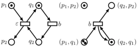
Figure 2 gives an example of a type-1 secure contraction. Notice that this contraction is not type-2 secure because M0(q 1) 6= 0. p1 ε p2 q1 q2 b (p1, p2) b (p1, q1) (q2, p2) (q2, q1)
Fig. 2: A Petri net with one silent transition (left) and the Petri net obtained by contraction of this transition (right).
If N is a safe labelled Petri net then its t-contraction is 2-bounded, but not necessarily safe. As we need to work with safe Petri nets (essentially because solutions to planning problems are found using unfolding techniques [5]) we are interested only in secure t-contractions preserving safeness. The proposition below gives a cheap sufficiency test for a contraction to be secure and safeness-preserving (it is obtained
by combination of the definition of secure given above with the sufficient conditions for safeness-preserving given in [18]). Proposition 3. A contraction of a transition t in a net N is secure and safeness-preserving if either
1) |t•| = 1,•(t•) = {t} and M0(p) = 0 with t•= {p}
2) |•t| = 1,•(t•) = {t} and ∀p ∈ t•, M0(p) = 0; or 3) |•t| = 1 and (•t)•= {t};
There exists a full characterisation of safeness-preserving contractions as a model checking problem [18]. However, testing it is much more expensive, so we do not consider it.
2) Redundant transitions and places: It may be the case (in particular after performing some silent transition contractions) that the Petri net contains redundant transitions and places. Removing them reduces the size of the net, while preserving its language and safeness [18].
A transition t in a labelled Petri net N = (P, T, F, M0, Λ, λ) is redundant if either
• it is a loop-only transition: an ε-transition such that
F ((p, t)) = F ((t, p)) for each p ∈ P ; or
• it is a duplicate transition: there is another transition t0 such that λ(t) = λ(t0), and F ((p, t)) = F ((p, t0)) and F ((t, p)) = F ((t0, p)) for each p ∈ P .
The set of all redundant places of a Petri net can be fully characterised by a set of linear equations [11] that we do not describe here. Examples of redundant places in safe Petri nets are:
• duplicate places: p is a duplicate of q if M0(p) = M0(q),
F (t, p) = F (t, q) and F (p, t) = F (q, t) for all t;
• loop-only places: p is a loop-only place if F (t, p) =
F (p, t) for all t and M0(p) > 0.
3) Algorithmic description of the suggested projection op-eration: Using the reductions described above we implement the projection operation as a re-labelling of the corresponding transitions by ε as described in Section III-B, followed by (secure, safeness preserving) transition contractions and re-dundant places/transitions removing while it is possible.
Note that there is no guarantee that all the silent transitions are removed from a Petri net. Moreover, depending on the order of the transition contractions and of the redundant places and transitions removing, the nets obtained may vary. Some guidelines about which silent transitions should be removed first are given in [18].
IV. EXPERIMENTAL EVALUATION
In order to show the practical interest of replacing automata by Petri nets in the message passing algorithms for factored planning we compared these two approaches on benchmarks. For that we used Corbett’s benchmarks [10]. Among these we selected the ones suitable to factored planning, that is the ones such that increasing the size of the problem increases the number of components rather than their size. This gave us five problems. They are not all living on trees so we had to merge some components (i.e. replace them by their product) in order to come up with trees and be able to run our algorithm.
Notice that the necessity of merging some components is an argument in favour of the use of Petri nets as there is usually local concurrency inside the new components obtained after merging. We first describe the five problems we considered and explain how we made each of them live on a tree. After that we give and comment our experimental results.
A. Presentation of the problems
a) Milner’s cyclic scheduler: A set of n schedulers are organised in a circle. They have to activate tasks on a set of n customers (one for each scheduler) in the cyclic order: customer i’s task must have started for the kth time before customer i + 1’s task starts for the kthtime. Each customer is a component, as well as each scheduler. Customer i interacts only with scheduler i while a scheduler interacts with its two neighbour schedulers. The interaction graph of this system is thus not a tree. We first make it a circle by merging each customer with its scheduler. After that we make it a tree (in fact a line) by merging the component i (customer i and scheduler i) with component n − i − 1.
b) Divide and conquer computation: A divide and con-quer computation using a fork/join principle. A bounded num-ber n of possible tasks is assumed. Each task, when activated, chooses (nondeterministically) to ”divide” the problem by forking (i.e. by activating the next task) and then doing a small computation, or to ”conquer” it by doing a bigger computation. Initially the first task is activated. The last task cannot fork. Each task is a component and their interaction graph is a line: each task interacts (by forking) with the next task and (by joining) with the previous task.
c) Dining philosophers: The classical dining philoso-phers problem where n philosophiloso-phers are around a table with one fork between each two philosophers. Each philosopher can perform four actions in a predetermined order: take the fork at its left, take the fork at its right, release the left fork, release the right fork. The components are the forks and the philosophers. Each philosopher shares actions with the two forks he can take, so the interaction graph of this problem is a circle. To make a tree from it we simply merge each philosopher with a fork as follows: philosopher 1 with fork n, philosopher 2 with fork n − 1, and so on.
d) Dining philosophers with dictionary: The same prob-lem as dining philosophers except that the philosophers also pass a dictionary around the table, preventing the philoso-pher holding it from taking forks. This changes the interac-tion graph as each philosopher now interacts with his two neighbour philosophers. To make it a tree we merge each philosopher with the corresponding fork (philosopher i with fork i) and then merge these new components as in the case of Milner’s scheduler.
e) Mutual exclusion protocol (Token ring mutex): A standard mutual exclusion protocol in which n users (each one associated with a different server) access a shared resource without conflict by passing a token around a circle formed by the servers (the server possessing the token enables access to the resource for its customer). Each user as well as each
server is a component. User i interacts with server i and each server interacts with the server before it and the server after it on the circle (by passing the token). The interaction graph of this system is not a tree. We merge each user with the corresponding server (user i with server i), making the interaction graph a circle. Then we use the same construction as in the case of Milner’s scheduler in order to make it a tree. B. Experimental results
We ran the message passing algorithm using a representation of the components as automata and as Petri nets. All our experiments were run on the same computer (Intel Core i5 processor, 8GB of memory) with a time limit of 50 minutes. Our objective was to compare the runtimes of both approaches, and in particular to see if they scale up well as problem sizes increase. The runtime of Algorithm 2 is negligible compared to Algorithm 1 so it is not shown on the charts.
0.01 0.1 1 10 100 1000 10000 20 40 60 80 100 120 140 160 180 200 time (s) number of tasks automata Petri nets
(a) Divide and conquer
0.01 0.1 1 10 100 1000 10000 20 40 60 80 100 120 140 160 180 200 time (s) number of philosophers automata Petri nets (b) Dining philosophers
Fig. 3: Problems where the representation of the components as automata is the best
Figure 3 presents the results obtained for the divide and conquer computation (3a) and for the dining philosophers problem (3b). For these two problems, the approach using automata scales up better than the approach using Petri nets. In order to explain this difference we looked at the size of the automata and of the Petri nets involved in the computations.
0.01 0.1 1 10 100 1000 10000 3 4 5 6 7 8 9 10 11 12 13 14 15 16 17 18 19 time (s) number of schedulers automata Petri nets
(a) Milner’s cyclic scheduler (small instances)
0.01 0.1 1 10 100 1000 10000 20 40 60 80 100 120 140 160 180 200 time (s) number of schedulers Petri nets
(b) Milner’s cyclic scheduler (larger instances)
0.01 0.1 1 10 100 1000 10000 3 4 5 6 7 8 9 10 11 12 13 14 15 16 17 18 19 time (s) number of philosophers automata Petri nets
(c) Dining philosophers with dictionary (small instances)
0.01 0.1 1 10 100 1000 10000 20 40 60 80 100 120 140 160 180 200 time (s) number of philosophers Petri nets
(d) Dining philosophers with dictionary (larger instances)
0.01 0.1 1 10 100 1000 10000 3 4 5 6 7 8 9 10 11 12 13 14 15 16 17 18 19 time (s) number of users automata Petri nets
(e) Token ring mutex (small instances)
0.01 0.1 1 10 100 1000 10000 20 40 60 80 100 120 140 160 180 200 time (s) number of users Petri nets
(f) Token ring mutex (larger instances)
It appeared that the size of the automata was not depending on the number of components. However, the size of the Petri nets was growing with the size of the problems. Looking more closely to these Petri nets we noticed that they were containing mostly silent transitions. Implementing more size reduction operations, in particular the ones based on unfolding techniques, may solve this issue.
Figure 4 shows the results obtained for the three other prob-lems: Milner’s cyclic scheduler (4a, 4b), the dining philoso-phers with a dictionary (4c, 4d), and the mutual exclusion protocol on a ring (4e, 4f). On these three problems the Petri nets approach scales up far better than the automata approach. In fact, only very small instances of these three problems can be solved using automata.
V. TOWARD COST-OPTIMAL PLANNING
This section shows how the previous factored planning approach could be adapted to cost-optimal planning. It first defines formally the cost-optimal factored planning problem in terms of weighted Petri nets. It then shows that the central no-tions of transition contraction and of redundant transition/place removal can be both extended to the setting of weighted Petri nets in some particular cases.
A. Cost-optimal planning and weighted Petri nets
In cost-optimal planning the objective is not only to find an execution leading to the goal, but to find a cheapest one. This notion of a best sequence can be defined by the means of costs associated with the transitions of a Petri net.
A weighted labelled Petri net is a tuple (P, T, F, M0, Λ, λ, c) where (P, T, F, M0, Λ, λ) is a labelled Petri net and c : T → R≥0 is a cost-function on transitions.
In such a Petri net, each execution o = t1. . . tn has a cost
c(o) = c(t1) + · · · + c(tn). The (weighted) language of a
weighted Petri net is then:
L(N ) = {(λ(o), c) | o ∈ hM0i, c = min
o0∈hM0i,λ(o0)=λ(o)c(o
0)}.
A cost-optimal planning problem is then defined as a pair (N, g) where N is a weighted labelled Petri net and g is a goal label. One has to find an execution o = t1. . . tnfrom the
initial marking of N , such that g appears exactly once at the end of the labelling of o and such that the cost of o is minimal among all similar executions in N .
B. Product of weighted Petri nets
As for factored planning problems, cost-optimal planning problems are defined using a notion of product of weighted labelled Petri nets.
The product N1 × N2 = (P, T, F, M0, Λ, λ, c) of two
weighted labelled Petri nets is defined as the product of the underlying labelled Petri nets, by assigning to the transitions resulting from a fusion the sum of costs of the original transitions (the transitions that did not participate in a fusion retain their original cost.)
A cost-optimal factored planning problem is then defined as a tuple N = (N1, . . . , Nn) of cost-optimal planning problems
((Pi, Ti, Fi, Mi0, Λi, λi, ci), g). One has to find a cost-optimal
solution to the problem (N1× · · · × Nn, g) without computing
the full product.
C. Message passing for cost-optimal factored planning The message passing algorithm can be used on weighted languages [14]. For that, the projection of a weighted language L (defined over Λ) to a sub-alphabet Λ0 is:
ΠΛ0(L) = {(w|Λ0, c) : (w, c) ∈ L, c = min
(w0,c0)∈L
w0|Λ0=w|Λ0
c0},
and the product of L1 and L2 (defined over Λ1 and Λ2
respectively) is:
L1× L2= {(w, c) : w ∈ Π−1Λ1∪Λ2( ¯L1) ∩ Π
−1
Λ1∪Λ2( ¯L2), c = c1+ c2 with(w|Λ1, c1) ∈ L1, (w|Λ2, c2) ∈ L2}, where ¯L is the support of the weighted language L:
¯
L = {w : ∃(w, c) ∈ L}.
Exactly as in the case of languages without weights one gets a method to find a cost-optimal word into a compound weighted language L = L1× · · · × Ln without computing
L as soon as L1, . . . , Ln lives on a tree. From the updated
components L0i obtained by Algorithm 1 one can extract this cost-optimal word of L using Algorithm 2, just replacing each selection of a word by the selection of a cost-optimal word. This is due to the fact that:
1) any cost-optimal word w with cost c in L is such that w|Λi is a cost-optimal word with the same cost c in L0
i= ΠΛi(L); and
2) for any cost-optimal word wi in L0i= ΠΛi(L) with cost c there exists a word w in L with the same cost c, which is also cost-optimal and satisfies wi= w|Λi.
Exactly as before we can show that the product of weighted Petri nets implements the product of weighted languages. Proposition 4. For any two weighted labelled Petri nets N1
and N2 one hasL(N1× N2) = L(N1) × L(N2).
Proof:From Proposition 1 one directly gets that L(N1×
N2) and L(N1) × L(N2) have the same support. It remains
to prove that for any (w, c) ∈ L(N1× N2) the corresponding
(w, c0) ∈ L(N1) × L(N2) is such that c = c0. For that assume
c < c0 (resp. c > c0) the construction of the proof of ⊆ (resp. ⊇) for Proposition 1 can be applied to construct an execution o in L(N1)×L(N2) (resp. L(N1×N2)) such that the labelling
of o is w and its cost is c (resp. c0), which is a contradiction with the fact that (w, c0) ∈ L(N1) × L(N2) (resp. (w, c) ∈
L(N1× N2)) because c0 > c (resp. c > c0) is not the minimal
cost for w in this net.
Similarly as for non-weighted Petri nets, the projection of a weighted labelled Petri net N = (P, T, F, M0, Λ, λ, c)
on an alphabet Λ0 is simply the weighted labelled Petri net ΠΛ0(N ) = (P, T, F, M0, Λ0, λ0, c) where
λ0(t) = λ(t) if λ(t) ∈ Λ0 = ε else.
Proposition 5. For any weighted labelled Petri net N and any alphabet Λ0, one hasL(Π
Λ0(N )) = ΠΛ0(L(N )).
Proof:The fact that L(ΠΛ0(N )) and ΠΛ0(L(N )) have the same support comes from Proposition 2. Observe that only the label of a transition may change during the projection, while its cost remains the same. Hence for any (w, c) ∈ L(ΠΛ0(N )) the corresponding (w, c0) ∈ ΠΛ0(L(N )) is such that c = c0, which concludes the proof.
This allows us to use weighted Petri nets in our message passing algorithm instead of weighted languages.
D. Efficient projection of weighted Petri nets
We conclude this part on cost-optimal planning by examin-ing when the size reduction operations (transition contraction, redundant places and transitions removal) can be applied to weighted Petri nets while preserving their weighted languages. 1) Removing redundant transitions and places: Loop-only transitions can be removed, exactly as in the case of non-weighted Petri nets. Indeed, consider any execution o = t1. . . tn of a Petri net N such that for some i ≤ n the
transition ti is loop-only. It is straightforward that o0 =
t1. . . ti−1ti+1. . . tn is also an execution of N . As ti is a
silent transition one gets λ(o) = λ(o0). Moreover c(ti) ≥ 0,
so c(o0) ≤ c(o). Hence, tiis not useful for defining words nor
their optimal costs.
Duplicate transitions can still be removed as well. When considering a transition t and its duplicate t0 one just has to take care to keep any one with the minimal cost. Indeed, consider any execution o = t1. . . tn of a Petri net N such
that for some i ≤ n the transition ti is a duplicate of some
transition t0i with a smaller cost. It is straightforward that o0 = t1. . . ti−1t0iti+1. . . tn is also an occurrence sequence
of N . As λ(ti) = λ(t0i) one gets λ(o) = λ(o0). And as
c(ti) ≥ c(t0i), c(o0) ≤ c(o). So, due to the existence of t0i, the
transition ti is not useful for defining words nor their optimal
costs.
Redundant places can be removed exactly as in the non-weighted case, as they do not affect the non-weighted language.
2) Contraction of silent transitions: We remark that, when a silent transition t is contracted, its cost has to be re-distributed to other transitions in the net, in order to ensure that costs of words in the net with t and costs of words in the net without t are the same. This first leads to the conclusion that silent transitions with cost 0 can be contracted exactly as in the non-weighted case.
From now on we consider only silent transitions t such that c(t) > 0. For an execution o and a set T0 of transitions, denote by |o|T0 the number of transitions from T0 in o. For a transition t with non-zero cost, if there exists a (non-empty) set T (t) of transitions (not containing t) such that for any execution o one has |o|T (t)= |o|{t}, then t can be contracted
and the cost of each transition of T (t) increased by c(t). This clearly preserves weighted languages. However, such a T (t) does not exist in general, as one can notice in the solid part of Figure 5: the execution t1does not contain the silent transition
t2, so t1∈ T (t/ 2), and then necessarily |t1t2|T (t)6= |t1t2|{t}.
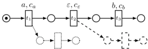
t1 a, ca t2 ε, cε t3 b, cb
Fig. 5: A Petri net with weights on transitions.
It is possible to relax the definition of T (t). Indeed, in a weighted language, only the best costs for words are considered, so it is sufficient to ensure that for any word w the executions o = arg minλ(o0)=wc(o0) are such that |o|T (t)= |o|{t}. Considering the net obtained by considering
only the solid part of Figure 5 one can then take T (t2) = {t3}.
Indeed, the word a is obtained with best cost from the execution t1 and the word ab from the execution t1t2t3, so
the execution t1t2 never has to be considered.
With that in mind we look at the different cases of secure and safeness preserving transition contractions, and see if some T (t) can be found in these cases. Three cases are possible.
First, if the considered transition t satisfies case 1 in Propo-sition 3 (safeness preservation), then one can take T (t) = (t•)•. Indeed, in this case, t• = {p} with M0(p) = 0 and
•(t•) = {t} so the transitions in (t•)•
can only be fired after a firing of t (they are not initially enabled and they can only be enabled by t) and at most one of them can be fired after each firing of t (because |t•| = 1 and •(t•) = {t}). Thus for
any execution o one has |o|T (t) ≤ |o|{t}. Moreover, for any
execution o achieving the minimal cost for the word λ(o) one has |o|T (t)≥ |o|{t}(else one occurrence of the silent transition
t can be removed from o without changing the obtained word, and thus o did not achieve the minimal cost for λ(o)).
Secondly, if t satisfies case 2 in Proposition 3 then for the same reasons as above the transitions in (t•)•can only be fired after firing t and for any execution o achieving the minimal cost for a word one has |o|(t•)•≥ |o|{t}. However, in general, it can be the case that |o|(t•)•> |o|{t}, because |t•| > 1 and so some transitions from (t•)• may be fired concurrently (as an example consider t3 and the dashed transition in Figure 5) or
sequentially without having to fire t another time. We thus take T (t) = (t•)• and limit these type-2 secure contractions to a simple case where only one transition in (t•)•can be fired after each occurrence of t: when ∀t0, t00∈ (t•)•
,•t0∩•t00∩ t•6= ∅.
Thirdly, if t satisfies case 3 in Proposition 3 then one cannot take T (t) = (t•)•, as it is possible that •(t•) ⊃ {t}, and so the transitions from (t•)• may be enabled without firing t before. Denote by p the only place in •t. Assume it is such that M0(p) = 0. Then, T (t) = •p is a reasonable candidate. Indeed, t can only be enabled by the firing of some transition in •p. However, there is no guarantee that the firing of a transition t0 ∈•p enforces to fire t afterwards (as an example
t1 is useful for firing the dotted transition in Figure 5), which
would be necessary if T (t) = •p. In the particular case of planning, one is not interested in the full language of a Petri net, but only in those words finishing by the special label g.
So one only needs that |o|T (t) = |o|{t} for the executions o
such that λ(o) ends by g. In this context one can thus allow contraction of transitions t (taking T (t) = •p) as soon as M0(p) = 0, and ∀t0 ∈ •p, λ(t0) 6= g and t0• = {p} (recall
that p•= {t}, so p enables only t). In the context of planning this ensures that t will always be fired after such t0 in an execution achieving the minimal cost for a word.
In summary, for each case where a transition can be removed while preserving safeness, one is able to give a sufficient condition for preserving also the costs of words that matter in the resolution of an optimal planning problem, i.e. those finishing by the special goal label g. In two cases however these conditions are more restrictive than in the non weighted case, when transition contraction has to preserve language and safeness only.
VI. CONCLUSION
This paper described an extension of a distributed planning approach proposed in [9], where the local plans of each component are represented as Petri nets rather than automata. This technical extension has three main advantages. First, Petri nets can represent and exploit the internal concurrency of each component. This frequently appears in practice, as factored planning must operate on interaction graphs that are trees, and getting back to this situation is naturally performed by grouping components (through a product operation), which creates internal concurrency. Secondly, the size reduction operations for Petri nets (transition contraction, removal of redundant places and transitions) are local operations: they do not modify the full net but only parts of it. By contrast, the size reduction operation for automata (minimisation) is expensive (while necessary [19]). As the performance of the proposed factored planning algorithm heavily depends on the ability to master the size of the objects that are handled, Petri nets allow us to deal with much larger components. Thirdly, the product of Petri nets is also less expensive than the product of automata. This again contributes to keeping the complexity of factored planning under control, and to reaching larger components.
This new approach was compared to its preceding version, based on automata computations (which has been previously successfully compared to a version of A* in [9]), on five benchmarks from [10] that were translated into factored plan-ning problems. For two of these benchmarks, the automata approach is the best, due to many silent transitions not being removed from the Petri nets. Still, the Petri nets approach scales up decently on these problems, allowing one to address large instances. On the remaining three benchmarks, the au-tomata approach could hardly deal with small instances, while the Petri nets version scaled up very well. We believe that these experimental results (and in particular the three outstanding ones) show the practical interest of our new approach to factored planning.
Finally we examined how far these ideas could be pushed to perform cost-optimal factored planning. Surprisingly, the extension is rather natural as the central operation of size
reduction for Petri nets can be adapted to the case of weighted Petri nets, with almost no increase in theoretical complexity. By contrast, when working with automata, the extension was much more demanding: the minimisation of weighted automata has a greater complexity than for standard automata, and may even not be possible.
As future work, we will implement and evaluate the interest of cost-optimal factored planning based on weighted Petri nets, with a specific focus on the contraction of silent weighted transitions. In particular we want to investigate whether the conditions for contraction are too restrictive for an effective size reduction of Petri nets. It would also be interesting to see to which extent these conditions can be relaxed.
REFERENCES
[1] J. Esparza and K. Heljanko, Unfoldings – A Partial-Order Approach to Model Checking. Springer, 2008.
[2] A. Blum and M. Furst, “Fast planning through planning graph analysis,” Artificial Intelligence, vol. 90, no. 1-2, pp. 281–300, 1995.
[3] V. Khomenko, A. Kondratyev, M. Koutny, and W. Vogler, “Merged processes: A new condensed representation of petri net behaviour,” Acta Informatica, vol. 43, no. 5, pp. 307–330, 2006.
[4] E. Fabre, “Trellis processes: A compact representation for runs of concurent systems,” Discrete Event Dynamic Systems, vol. 17, no. 3, pp. 267–306, 2007.
[5] S. Hickmott, J. Rintanen, S. Thi´ebaux, and L. White, “Planning via Petri net unfolding,” in Proceedings of the 19th International Joint Conference on Artificial Intelligence, 2007, pp. 1904–1911.
[6] B. Bonet, P. Haslum, S. Hickmott, and S. Thi´ebaux, “Directed unfolding of Petri nets,” Transactions on Petri Nets and other Models of Concur-rency, vol. 1, no. 1, pp. 172–198, 2008.
[7] E. Amir and B. Engelhardt, “Factored planning,” in Proceedings of the 18th International Joint Conference on Artificial Intelligence, 2003, pp. 929–935.
[8] R. Brafman and C. Domshlak, “From one to many: Planning for loosely coupled multi-agent systems,” in Proceedings of the 18th International Conference on Automated Planning and Scheduling, 2008, pp. 28–35. [9] E. Fabre, L. Jezequel, P. Haslum, and S. Thi´ebaux, “Cost-optimal
factored planning: Promises and pitfalls,” in Proceedings of the 20th International Conference on Automated Planning and Scheduling, 2010, pp. 65–72.
[10] J. C. Corbett, “Evaluating deadlock detection methods for concurrent software,” IEEE Transactions on Software Engineering, vol. 22, pp. 161– 180, 1996.
[11] W. Vogler and B. Kangsah, “Improved decomposition of signal transition graphs,” Fundamenta Informaticae, vol. 78, no. 1, pp. 161–197, 2007. [12] P. Hart, N. Nilsson, and B. Raphael, “A formal basis for the heuristic
determination of minimum cost paths,” IEEE Transactions on Systems Science and Cybernetics, vol. 4, no. 2, pp. 100–107, 1968.
[13] J. Esparza, S. Romer, and W. Vogler, “An improvement of McMillan’s unfolding algorithm,” Formal Methods in System Design, vol. 20, no. 3, pp. 285–310, 1996.
[14] E. Fabre and L. Jezequel, “Distributed optimal planning: an approach by weighted automata calculus,” in Proceedings of the 48th IEEE Conference on Decision and Control, 2009, pp. 211–216.
[15] E. Fabre, “Bayesian networks of dynamic systems,” Habilitation `a Diriger des Recherches, Universit´e de Rennes1, 2007.
[16] V. Khomenko, M. Schaefer, and W. Vogler, “Output-determinacy and asynchronous circuit synthesis,” Fundamenta Informaticae, vol. 88, no. 4, pp. 541–579, 2008.
[17] C. Andr´e, “Structural transformations giving b-equivalent pt-nets,” in Proceedings of the 3rd European Workshop on Applications and Theory of Petri Nets, 1982, pp. 14–28.
[18] V. Khomenko, M. Schaefer, W. Vogler, and R. Wollowski, “STG decom-position strategies in combination with unfolding,” Acta Informatica, vol. 46, no. 6, pp. 433–474, 2009.
[19] L. Jezequel, “Distributed cost-optimal planning,” Ph.D. dissertation, ENS Cachan, 2012.