Implementation of Sources in an Energy-Stress Tensor Based Diffuse Sound Field Model

HAL Id: hal-02495516

https://hal.archives-ouvertes.fr/hal-02495516

Submitted on 2 Mar 2020

HAL is a multi-disciplinary open access

archive for the deposit and dissemination of sci-entific research documents, whether they are pub-lished or not. The documents may come from teaching and research institutions in France or abroad, or from public or private research centers.

L’archive ouverte pluridisciplinaire HAL, est destinée au dépôt et à la diffusion de documents scientifiques de niveau recherche, publiés ou non, émanant des établissements d’enseignement et de recherche français ou étrangers, des laboratoires publics ou privés.

Implementation of Sources in an Energy-Stress Tensor

Based Diffuse Sound Field Model

Aidan Meacham, Roland Badeau, Jean-Dominique Polack

To cite this version:

Aidan Meacham, Roland Badeau, Jean-Dominique Polack. Implementation of Sources in an Energy-Stress Tensor Based Diffuse Sound Field Model. International Symposium on Room Acoustics, Sep 2019, Amsterdam, Netherlands. �10.18154/RWTH-CONV-240108�. �hal-02495516�

Implementation of Sources in an Energy-Stress Tensor Based

Diffuse Sound Field Model

Aidan MEACHAM(1); Roland BADEAU(2); Jean-Dominique POLACK(1)

1_{Sorbonne Université, UMR CNRS 7190, Institut Jean le Rond∂’Alembert, France} 2_{LTCI, Télécom Paris, Institut Polytechnique de Paris, France}

ABSTRACT

An implementation of acoustic sources is developed in the context of an energetic wave equation derived from the energy-stress tensor, examined in the one-dimensional case [Dujourdy et al, Acta Acustica united with Acustica 103:480-491, 2017]. The method efficiently models diffuse sound fields that dom-inate reverberation at higher frequencies and larger distances. Monopole and dipole electroacoustical sources are considered. Using loudspeaker models rather than idealized distributions of sound energy allows for a convenient structure to evaluate directional dependence and frequency dependence for a variety of source types. Compared to initial condition formulations, an explicit source term enables real-istic modeling of complex sound sources with the possibility of spatial changes in time. A finite volume time domain (FVTD) approach is utilized to lay the groundwork for future extensions to three dimen-sions. The spatially invariant model parameters are determined iteratively by comparison with in situ measurements of a long hallway for both the monopole and dipole case in order to verify the validity of the framework.

Keywords: Room acoustics, finite difference methods, diffuse field

1. INTRODUCTION

Previous work, focused on an energetic wave equation based method for simulating room acous-tics, has relied upon bespoke dimensional reduction for tractability. While this approach developed by Dujourdy et al. (1, 2) has been successful in 1- and 2-dimensional contexts, the extension to 3 dimensions presents a challenge.

This energetic wave equation has been found to accurately model the statistical late reverberation, or diffuse field, resulting from an initial perturbation. Originating from Ollendorff and Picaut’s work (3, 4), it takes advantage of an additional degree of freedom given by the inclusion of a diffusion coefficient in addition to the traditional absorption coefficient resulting from deriving a wave equation based on the energy density and sound intensity rather than pressure and velocity. The main reason to consider this model over more traditional finite difference schemes is that it is highly efficient, both because the element sizes can be very large while still capturing relevant behavior, and because the late reverberation as predicted by more fine-grained models tends to be sensitive to perturbations that result from non-physical modeling phenomena such as dithering.

These solutions used finite difference time domain (FDTD) techniques to numerically model the resulting systems, a common formalism for discretizing partial differential equations. Recently, finite volume time domain (FVTD) approaches have become more popular since they allow for unstruc-tured meshes and also provide convenient machinery to confirm that conserved values are in fact accounted for in terms of storage and dissipation (5). Furthermore, they provide a straightforward programmatic framework that can accommodate 1-, 2-, or 3-dimensional problems with little change in structure.

In many acoustic FDTD or FVTD models, it is common to examine an unforced system where the evolution of acoustical phenomena through time is determined only by the initial distribution of pressure and velocity. This is a convenient formulation in the case where the model will be used to generate an impulse response, as an idealized omnidirectional source can be simply represented, often with a spatial Gaussian. There are some cases where it is useful to consider the forced system,

however, where source terms are included in the wave equation. Some examples of behavior that is more readily modeled by this approach include feedback or cases when the source position or directivity change over time.

In this study, we lay the groundwork for extending the energetic wave equation model to 3 di-mensions in the FVTD formalism by recontextualizing a 1-dimensional problem, while also consid-ering sources of acoustic energy other than initial conditions in order to accommodate many types of sources.

2. THEORY

2.1 Definitions

Following directly from Dujourdy et al. (1), we begin from a common acoustical model, _c12∂ttΨ −

∆Ψ = 0. The velocity potential Ψ is defined by v = −∇Ψ and p = ρ ∂tΨ. In this system, the sound pressure and particle velocity vector are given by p and v respectively, ∇ is the gradient operator, ∆ the Laplacian operator, ρ the air density, and c the speed of sound. Finally, we notate ∂i and ∂ii the

first and second derivatives according to coordinate i respectively.

2.2 Volume velocity sources

In order to introduce sources to the energetic wave equation, we can proceed directly to Equation 8 from Dujourdy et al. (1), with the divergence operator (∇·):

1 c∂tEtt+ ∇ · J = 0, 1 c∂tJ + ∇ ·    Exx Eyx Ezx Exy Eyy Ezy Exz Eyz Ezz   = 0.

This system presents a relation between the energy density E =ρ 2(

1

c2|∂tΨ|2+|∇Ψ|2) and the sound

intensity J = −ρ∂tΨ∇Ψ/c as defined by Morse and Feshback (6), and the wave-stress symmetric

tensor as defined by Morse (7) with components Eii=ρ₂(_c12|∂tΨ|2+ ∑jαi j|∂jΨ|2) or Ei j= ρ∂iΨ∂jΨ

for i, j = x, y, z with αi j= 1 when i = j or -1 otherwise.

Dimensional analysis shows that we can represent sources in the wave equation with the inclu-sion of source terms on the right hand side of each part that approximate the effects of a moving membrane in the acoustic space.

If Q is the volume velocity of a source, and p and v are the pressure and particle velocity immediately in front of that source, we can write

1 c∂tEtt+ ∇ · J = P = pQ c , 1 c∂tJ + ∇ ·    Exx Eyx Ezx Exy Eyy Ezy Exz Eyz Ezz   = Q = ρvQ . (1)

When the surface of the source moves into the volume of the room, Q and p are positive, and v (which is in the same direction as Q by continuity) on the surface is counted positively when the inward normal of the source surface into the room is orientated toward the positive X-axis. In order to account for a variety of source types and topologies, the pressure in front of a given source can be calculated in terms of frequency dependent characteristics such as the Thiele-Small parameters, the radiation impedance of a single driver, or the mutual impedance of an enclosure with multiple drivers. We note that this approach is an anechoic approximation to the impedance problem, as the reverberation within the space or other sources also contributes to the pressure in front of a given radiating structure, creating a coupled system. One justifying explanation is that in the frequency range we are expecting to model (generally above the Schroeder frequency), the free-field radiation impedance dominates, and thus we are free to treat sources individually and without considering the local acoustic conditions.

For a monopole source, Q and p have the same sign on both sides of the source, so P is positive. On the other hand, v points in opposite direction on either side of the source such that |Q| is zero.

For a dipole source such as an open baffle loudspeaker, Q , p, and v all have opposite signs on each side of the radiating surface. As a result, both P and Q are positive, with |Q| = P . Of course, dipole sources also imply particular frequency response effects that can be applied according to the frequency range of a given simulation.

For other types of non-idealized directional sources, directional radiation along the primary axes can be introduced according to near-field analysis of the source topology and geometry. Thus, mod-eling a sealed enclosure loudspeaker with a single driver, for example, would account for diffractive effects around the cabinet via contributions to Q corresponding to the principal axes of the wave-stress tensor.

Favorably, this description allows for a wide variety of sources, and can accommodate any system that can be parametrized in terms of its volume velocity output. While these extensions will not be addressed in this work, it is ostensibly possible to include arbitrary loudspeaker designs or other environmental sound sources. Thus, any collection of electromechanical devices can be represented in the model, which can be especially useful in predicting the behavior of sound reinforcement systems in enclosed spaces, for example.

2.3 FVTD model - spatial discretization

In order to proceed with a spatial discretization of this model, we note the similarity of these equations, which are denoted in terms of energy density and sound intensity, with the wave equation as written in terms of pressure and velocity:

1

ρ c2∂tp+ ∇ · v = 0, ρ ∂tv + ∇p = 0.

In the present case, we explore a quasi-one-dimensional case in order to utilize previously sug-gested dimensional reductions to account for the off-diagonal terms in the wave-stress tensor E for agreement with the scalar p. Otherwise, to physical constants, the systems exhibit identical behavior, so we can directly use a generalized FVTD formulation by inspection, replacing p and v with E and J. In this work, we refer specifically to the straightforward development in Bilbao et al. (8).

The space to be analyzed is a long hallway aligned on the X-axis of length lx, with width

and height ly, lz lx. We discretize the hallway into N identical rectangular solids Ωj (of volume

V = lxlylz/N) associated with average energy densities Ej and outward sound intensities Jjk and Jl,

depending if the intensity in question is incident upon another cell or a boundary. The distance be-tween centroids of each cell is thus h = lx/N, and since the hallway model has a constant section,

the surfaces between cells are identical (of area S = lylz) and the Nb boundary surfaces take on one

of three areas depending on their normal direction (lxly/N, lxlz/N, or lylz, indexed as Sl below).

Finally, we can integrate the total P over each cell and average Q over each outward surface to arrive at indexed quantities Pj and Qjk.

Rewriting Bilbao et al. (8) Equation 15 directly in terms of energy density and sound intensity, introducing terms for the wave-stress tensor, and including the previously derived source terms from Equation 1 results in V c dEj dt + N

∑

∑

∑

where βjk and γjl are indicator functions that are 1 if a given cell Ωj shares a face with another cell

Ωk or face on the boundary Sl, and 0 otherwise. Additionally, ζjkl is an indicator function for a cell,

boundary, and a neighboring cell that has a boundary that shares vertices with the first (“neighboring” boundaries, so to speak). In the configuration of cells under study, this indicator function adds eight terms for each cell that is not at an end - four times each for its neighbor in the positive and negative X direction - since all four of its boundaries (walls, ceiling, and floor) share vertices with

its neighbors’ boundaries. In general, this term acts to bidirectionally damp the transfer of energy between cells through the sound intensity terms as an approximation of diffusion. One interpretation of this effect is that it acts to reduce the specularity of reflections that typically facilitates energy transfer in the direction of wave propagation. In other words, sound intensity directed from one cell to another, where each has boundaries that share vertices with their common surface, acts to reduce the energy transfer through that common surface.

We assume, as before, that sound is propagating in the X direction, where E and Jx are constant

on a given section of the corridor, Jy is independent of z, and Jzis independent of y. This assumption

is borne out by the decision to discretize the hallway into a single line of cells, since the energy can only transfer in between neighboring cells and the boundaries. Then, using the energy balance J= AE/4 and the momentum balance Exy= DJ/4 from Equations 12 and 21 in Dujourdy et al. (1)

with the modified absorption and diffusion coefficients A and D, we can replace the outward normal sound intensities incident on a boundary and the energy densities in front of diffracting boundaries to arrive at V c dEj dt + N

∑

∑

∑

where Ejl indicates the energy density of a cell in front of a particular boundary surface.

One advantage of this approach, over integrating the boundary conditions on the walls and ceil-ings into a one-dimensional difference equation along the X-axis and solving for more complicated boundary conditions at the ends of the hallway, is that it allows us to apply simple boundary condi-tions at every discretized boundary while observing the same behavior as the previous model, with the side benefit of simplifying the implementation of spatial variance in the hallway (even though we will not consider such cases in this study).

Typically, FVTD approaches are used in cases where the boundaries are irregular, resulting in the need for unstructured elements. Of course, that is not the case here, such that the eventual implementation is a typical FDTD scheme over a structured grid. Nonetheless, it is convenient to proceed with the FVTD formulation since it provides a convenient formalism for examining the conservation of quantities that correspond to energy in a classic pressure-velocity wave equation. This context allows us to reason about the physical meaning of exchanges between energy density and sound intensity.

2.4 FVTD model - temporal discretization

From the formulation above, we can discretize the elements that are continuous in time by ap-proximating the temporal derivatives with temporal differences evaluated at a given sampling rate. The main advantage of the energetic wave equation model is that the modulation frequency of the late energy decay is very low, which implies that the spatial sampling step can be very large and the temporal sample rate can be low as well. This is in contrast to typical pressure and velocity wave equation approaches, where the goal is to resolve the highest frequency, leading to smaller discretization steps temporally and spatially, and thus, to simulations that are difficult to run in real time, even with accelerated processing (that may take place on a GPU, for example).

In terms of implementation, these conclusions justify the earlier decision to discretize the hallway into very large cells that do not require multiple divisions along the width and height, and can therefore utilize the one-dimensional approximations discussed earlier. Were this not the case, the difference equations relating neighboring cells would need to be more complicated in order to deal with the full wave-stress tensor, and the simplifications made for the boundary conditions would also not be valid.

With a discrete time step T such that fn= f (nT ) is a discrete time approximation of the contin-uous time series f (t), we introduce the forward and backward shift operators e+fn= fn+1, e−fn=

fn−1, the forward and backward difference operators δ+ = (e+− 1)/T, δ− = (1 − e−)/T , and the

forward and backward averaging operators µ+ = (e++ 1)/2, µ−= (e−+ 1)/2. Then, by replacing

the continuous derivatives in Equation 3 with interleaved approximations of the energy density and sound intensity (as in Bilbao et al. (8) Section IV), a fully discrete version of Equation 3 including

the source terms can be written as V cδ+Ej+ N

∑

∑

∑

where Pj and Qjk are aligned in time with Jjk and Ej respectively, and we introduce temporal

aver-aging to preserve the time alignment and differential relationship in each equation.

Then, using the notation e±f = f±, expanding the temporal operators, and solving for E+j and

Jjk: E+_j =Ej(1 − cT V ∑ Nb l=1γjlSlA₈) +cT_V Pj−cT_V ∑Nk=1βjkSJjk 1 +cT_V ∑N_l=1b γjlSlA₈ , Jjk= J−_jk(1 − ∑Nb l=1ζjklS_VlcTD₈) + cT Qjk+cT_h (Ej− Ek) 1 + ∑Nb l=1ζjklS_VlcTD₈ . (5)

This is a realizable two-step FVTD scheme.

Thus, in order to integrate arbitrary source material, the output from the loudspeaker model is bandpass filtered to the selected octave, converted to acoustic power, decimated to fit the much lower simulation sample rate, and injected into the cells corresponding to the position of the source. By repeating the process for multiple octave bands, a full-band response can be synthesized, though it is important to note that an auralization scheme for these results has not yet been realized. Of course, the inclusion of the source in these equations does not preclude also accounting for initial conditions, which may be set just as before by directly specifying the energy density and sound intensity at the first two time steps.

3. FITTING MODEL PARAMETERS TO MEASUREMENTS

Figure 1 – Floorplan for the corridor under consideration.

3.1 Room geometry

The hallway we examined for this study had an overall length of 45 m, with a width of 1.59 m and a height of 2.375 m. A plan of the corridor can be seen in Figure 1. In the main narrow portion of the hallway, the ceiling height was measured to a fine metal grating suspended below the actual height of the corridor, which carried lighting and conduit. The hard ceiling was 3.26 m, with a decrease every 1.5 m for metal support beams to 2.8 m.

In the recesses, all of which were of uniform length and depth (except for the doorway furthest on the right of the plan), the width increased to 2.39 m and the height decreased to 2.2 m, and ceiling was masonry rather than the grating mentioned above. In some of the recesses, there were glass display cases or small pieces of furniture that contributed to the diffusive effects of the recesses themselves. The entire floor was linoleum, and for the most part, the walls were wooden panel and masonry. There were occasional vertical metal gratings on the flat wall over shallow indentations. The HVAC was audible but not distracting, and did not present an obstacle for the calculation of acoustical indices. All doors entering the hallway were closed, and the doors in the center of the hallway were fully open.

3.2 Measurements

Impulse responses were collected using a SoundField ST250 microphone and an Outline GRS omnidirectional speaker, with a MOTU Traveler sound card. The source was positioned 1 meter away from the right end of the hall in Figure 1, 1.5 m above the ground, and centered between the two walls. Measurements were collected with the microphone’s X-axis aligned along the length of the hallway at distances of 4, 8, 12, and 16 m from the source. For one set of recordings, all of the speaker drivers were active, approximating a point source, and for a second set, only the sets of 3 speakers aligned along the X-axis were activated (in groups of 3), with opposite phases, to approx-imate a dipole source. Recordings were made using the swept sine method (9, 10) as implemented in the Adobe Audition plugin Aurora. The sweep length was 20 seconds, and the source level was adjusted digitally to maximize the signal-to-noise ratio without clipping. All gains were recorded in order to recover the relative energy level at each measurement location. The sweep responses were then post-processed by convolution with the inverse sweep to recover impulse responses for each location and source type.

In order to determine the frequency ranges that could be fit by the model, each impulse response was filtered into bandlimited responses using a standard octave-band filterbank, and then the desired metrics were calculated for each resulting frequency band. The T60 (a measure of temporal decay)

was calculated by a linear fit to the Energy Decay Curve in dB for each frequency band and at each receiver location. This is sometimes known as Schroeder’s reverse integration (11). Next, each receiver location was averaged to arrive at a single T60 for the entire hallway in each band. Finally,

spatial decays (similar to strength of sound, or G) were calculated by a linear fit to the sum of energy for each band-limited response across each receiver location.

3.3 Simulation results

In order to verify the reformulation of the model in the FVTD formalism, we ran initial-value problem simulations for all combinations of modified absorption and scattering coefficients A and D. We discretely sampled each variable with enough resolution to confidently resolve the changes in the derived temporal and spatial measures mentioned above. The initial conditions were chosen to be a temporal Gaussian, centered at the same location as the source, in order to minimize spurious numerical oscillations. The sample rate was chosen to fit the stability criterion given in Bilbao et al. (8).

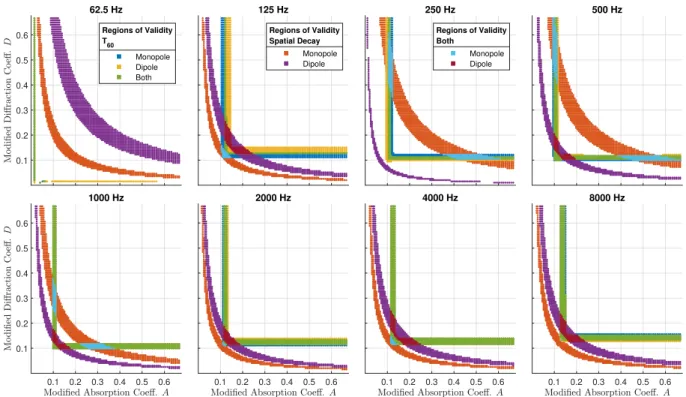
We then compared the results to the physically collected bandlimited impulse responses. We sug-gest that the subset of simulations whose measures fall within 10% of the in situ indices sufficiently model the desired acoustical characteristic. For each measure, those combinations of coefficients that fall within this range form a contiguous band in the search space which we will refer to as a “region of validity.”

In the interest of space, we have presented the results of fitting both the monopole and dipole source on the same set of graphs in Figure 2, organized by octave band. Each color indicates a region of validity for the specified measure. Thus, we have highlighted the regions where the T60

was within 10%, the regions where the spatial decay was within 10%, and the regions where both spatial and temporal characteristics were within 10% of the measured data. Simulations that satisfy this final category indicate whether the model is ultimately successful for each source type and octave band, and is the intersection of the regions of validity for both T60 and spatial decay. In short, those

combinations of coefficients are capable of successfully representing the stochastic reverberant field in the space for the given octave band.

For this set of measurements, it can be seen that the monopole case is valid above 125 Hz and the dipole case is valid above 500 Hz (since it could not be matched at 250 Hz). As expected, neither case is valid at 62.5 Hz. Interestingly, in every other band, many simulations were able to satisfy T60 for both the monopole and dipole cases, but in no case was a single simulation capable

of modeling the spatial decay for both source types.

By verifying that the model reproduces the desired behavior in the impulsive case, the plausi-bility of steady-state and time varying cases are also confirmed. Therefore, by using the derived parameters, it is possible to approximate the playback of arbitrary source material in the space for combinations of monopole and dipole sources with the appropriate values of P and Q. It is impor-tant to note that the findings of this exercise are not proof that the model is capable of representing an arbitrary space, nor can the derived coefficients be used for other spaces, but serve as validation of the model in this specific instance, and for spaces similar to the selected hallway in terms of geometric, absorptive, and diffusive characteristics.

0.1 0.2 0.3 0.4 0.5 0.6 62.5 Hz Monopole Dipole Both Regions of Validity T₆₀ 125 Hz Monopole Dipole Regions of Validity Spatial Decay 250 Hz Monopole Dipole Regions of Validity Both 500 Hz 0.1 0.2 0.3 0.4 0.5 0.6 0.1 0.2 0.3 0.4 0.5 0.6 1000 Hz 0.1 0.2 0.3 0.4 0.5 0.6 2000 Hz 0.1 0.2 0.3 0.4 0.5 0.6 4000 Hz 0.1 0.2 0.3 0.4 0.5 0.6 8000 Hz

Figure 2 – Agreement between simulated and measured data for the monopole and dipole configurations in each frequency band.

4. CONCLUSIONS AND FUTURE WORK

In this work, we have reimplemented a one-dimensional solution for the wave-stress tensor based wave equation with the addition of arbitrary sources. We compared a range of simulations to physical measurements in a long hallway to show that it is possible to fit boundary conditions that model the acoustic behavior of both monopole and dipole sources.

For the most part, the point of this work has been to prepare a framework that could facilitate extension of the model to three dimensions. While the acoustic behavior immediately in front of boundaries is well represented by the model, wave propagation in free space is not, and therefore must be addressed with a separate method, such as ray tracing or a different FDTD/FVTD scheme. Doing so implies questions about the process of acoustic transfer between the two systems, as well as the necessary thickness of a translation layer between the two problem domains. Furthermore, it is important to consider how the model deals with more realistic cases where diffusion and absorption are not spread evenly over all surfaces.

As mentioned earlier, we omitted acoustic feedback in the source representation for simplicity. Future work may consider the relationship of the energy density to the calculation of radiation impedance in order to realize a more accurate coupled model without the anechoic approximation, including effects from multiple sources.

Though this reformulation of the one-dimensional problem gives similar results to the previous Telegrapher’s equation solution, when the modified absorption and diffusion coefficients A and D are close in value, the simulations show oscillations that complicated the evaluation of temporal and spatial measures. Fortunately, it was possible to extract indices for all relevant simulations to facilitate the evaluation of the method, but this behavior should be examined more closely.

While all of the implementations until now have required calibration against real measurements in order to model a space, the model can not be used as a prediction tool in the general case until a systematized method for generating simulation parameters from spatial geometry and materials properties can be demonstrated. What such a method would require in order to capture the conditions for a given space (in either the homogeneous or non-homogeneous case) is as of yet unknown.

Finally, further experiments can be performed to evaluate the real-time performance of the method for predicting reverberation given arbitrary source material or more complex loudspeaker configura-tions given the significant computational advantages of the large element sizes and low sample rate requirements.

REFERENCES

1. Dujourdy H, Pialot B, Toulemonde T, and Polack JD. An Energetic Wave Equation for Mod-elling Diffuse Sound Fields – Application to Corridors. Acta Acustica united with Acustica 2017;103:480–91.

2. Dujourdy H, Pialot B, Toulemonde T, and Polack JD. An Energetic Wave Equation for Mod-elling Diffuse Sound Fields—Application to Open Offices. Wave Motion. Innovations in Wave Modelling II 2019;87:193–212.

3. Ollendorff F. Statistical Room-Acoustics as a Problem of Diffusion (A Proposal). Acta Acustica united with Acustica 1969;21:236–45.

4. Picaut J, Simon L, and Polack JD. A Mathematical Model of Diffuse Sound Field Based on a Diffusion Equation. Acta Acustica united with Acustica 1997;83:614–21.

5. Bilbao S. Modeling of Complex Geometries and Boundary Conditions in Finite Difference/Fi-nite Volume Time Domain Room Acoustics Simulation. IEEE Transactions on Audio, Speech, and Language Processing 2013;21:1524–33.

6. Morse PM and Feshbach H. Methods of Theoretical Physics. Mc Graw-Hill Book Company, 1953.

7. Morse PM and Ingard KU. Theoretical Acoustics. Princeton University Press, 1968. 949 pp. 8. Bilbao S, Hamilton B, Botts J, and Savioja L. Finite Volume Time Domain Room Acoustics

Simulation under General Impedance Boundary Conditions. IEEE/ACM Transactions on Audio, Speech, and Language Processing 2016;24:161–73.

9. Farina A. Simultaneous Measurement of Impulse Response and Distortion with a Swept-Sine Technique. In: Audio Engineering Society Convention 108. Audio Engineering Society, 2000. 10. Farina A. Advancements in Impulse Response Measurements by Sine Sweeps. In: Audio

Engi-neering Society Convention 122. Audio EngiEngi-neering Society, 2007:21.

11. Schroeder MR. New Method of Measuring Reverberation Time. The Journal of the Acoustical Society of America 1965;37:409–12.