HAL Id: hal-01735612
https://hal.archives-ouvertes.fr/hal-01735612
Submitted on 25 Oct 2018HAL is a multi-disciplinary open access
archive for the deposit and dissemination of sci-entific research documents, whether they are pub-lished or not. The documents may come from teaching and research institutions in France or abroad, or from public or private research centers.
L’archive ouverte pluridisciplinaire HAL, est destinée au dépôt et à la diffusion de documents scientifiques de niveau recherche, publiés ou non, émanant des établissements d’enseignement et de recherche français ou étrangers, des laboratoires publics ou privés.
Integrating uncertainties to the combined environmental
and economic assessment of algal biorefineries: A Monte
Carlo approach
Paula Perez-Lopez, Mahdokht Montazeri, Gumersindo Feijoo, Maria Teresa
Moreira, Matthew Eckelman
To cite this version:
Paula Perez-Lopez, Mahdokht Montazeri, Gumersindo Feijoo, Maria Teresa Moreira, Matthew Eck-elman. Integrating uncertainties to the combined environmental and economic assessment of algal biorefineries: A Monte Carlo approach. Science of the Total Environment, Elsevier, 2018, 626, pp.762 - 775. �10.1016/j.scitotenv.2017.12.339�. �hal-01735612�
Integrating uncertainties to the combined environmental and
economic assessment of algal biorefineries: a Monte Carlo
approach
Paula Pérez-López1,2*, Mahdokht Montazeri3, Gumersindo Feijoo1, María Teresa Moreira1, Matthew J. Eckelman3
1 Department of Chemical Engineering, Institute of Technology, University of Santiago de
Compostela, 15782, Santiago de Compostela, Spain
2 Present address: MINES ParisTech, PSL Research University, Centre Observation, Impacts,
Energie (O.I.E.), 1 rue Claude Daunesse CS 10207, 06904 Sophia Antipolis Cedex, France
3 Department of Civil and Environmental Engineering, Northeastern University, 360 Huntington
Avenue, Boston, MA 02115, USA.
* Corresponding author: Tel.: +33 4 97 15 70 55; E-mail address: paula.perez_lopez@mines-paristech.fr
ABSTRACT
The economic and environmental performance of microalgal processes has been widely analyzed in recent years. However, few studies propose an integrated process-based approach to evaluate economic and environmental indicators simultaneously. Biodiesel is usually the single product and the effect of environmental benefits of co-products obtained in the process is rarely discussed. In addition, there is wide variation of the results due to inherent variability of some parameters as well as different assumptions in the models and limited knowledge about the processes. In this study, two standardized models were combined to provide an integrated simulation tool allowing the simultaneous estimation of economic and environmental indicators from a unique set of input parameters. First, a harmonized scenario was assessed to validate the
assessments. In a second stage, a Monte Carlo simulation was applied to evaluate the influence of variable and uncertain parameters in the model output, as well as the correlations between the different outputs. The simulation showed a high probability of achieving favorable environmental performance for the evaluated categories and a minimum selling price ranging from $11 gal-1 to $106 gal-1. Greenhouse gas emissions and minimum selling price were found to have the
strongest positive linear relationship, whereas eutrophication showed weak correlations with the other indicators (namely greenhouse gas emissions, cumulative energy demand and minimum selling price). Process parameters (especially biomass productivity and lipid content) were the main source of variation, whereas uncertainties linked to the characterization methods and economic parameters had limited effect on the results.
GRAPHICAL ABSTRACT
KEYWORDS: microalgal biodiesel; life cycle assessment; economic assessment; uncertainty
1. Introduction
The potential of microalgal products and particularly bioenergy is widely recognized (Collet et al., 2014; Davis et al., 2011; Wijffels and Barbosa, 2010). However, the environmental feasibility is still subject to further optimization for the reduction of energy and fertilizer consumption, as well as to the development of novel eco-efficient technologies for algae processing (Collet et al., 2014). Moreover, there is a great controversy about the economic viability of large-scale algae production in the short-term (Davis et al., 2011; Richardson et al.; 2012).
Life cycle assessment (LCA) is the most widespread tool addressing the environmental aspects of microalgal processes. The production of bioenergy, especially in the form of biodiesel, has been the most common focus among the large number of LCA studies (Brentner et al., 2011; Campbell et al., 2011; Clarens et al., 2010; Collet et al., 2014; Draaisma et al., 2013; Montazeri et al., 2016; Sills et al., 2013; Woertz et al., 2014, Zaimes and Khanna, 2013). Most studies evaluate impact categories related to greenhouse gas emissions (GHG) and energy consumption (Brentner et al., 2011; Clarens et al., 2010; Collet et al., 2015; Draaisma et al., 2013; Sills et al., 2013; Woertz et al., 2014; Zaimes and Khanna, 2013). Energy balance can be analyzed in terms of cumulative energy demand (CED, i.e. total primary energy consumed or generated throughout the process)
(ERO(E)I, i.e. ratio between the total energy produced and the energy consumed in the process), also referred to as net energy ratio (Collet et al., 2015, Montazeri et al., 2016). Other common indicators include the eutrophication potential of the process, as well as land competition and water demand (Collet et al., 2015).
Recent works highlight the multi-functional nature of microalgal processes and the importance of co-product exploitation coupled to biofuel production, which may allow significant environmental benefits (Collet et al., 2015, Montazeri et al., 2016). Montazeri et al. (2016) suggest that the optimal environmental performance of biorefinery schemes is not necessarily associated with operating conditions that maximize lipid productivity (linked to the maximum biodiesel production), but with a balanced distribution of lipid and non-lipid fractions.
Techno-economic assessments of microalgal biorefineries are another essential element for the feasible implementation at large scale (Sun et al., 2011). Techno-economic models constitute key tools for the strategic planning and decision making process that help in the evaluation of project value (Borowitzka, 2013) and the decision about how and when to invest in commercial scale-up. Several studies on the economics of microalgal processes have been published in the last 30 years (Benemann and Oswald, 1996; Davis et al., 2011; 2014a; 2014b; Gong and You, 2014; Huntley and Redalje, 2007; Norsker et al., 2011; Richardson
One of the first and more detailed economic evaluations was the analysis by Benemann and Oswald (1996). This study provided a comprehensive estimate of capital and operating costs (per barrel, bbl, of oil produced) of the most common open pond designs and auxiliary elements (including downstream processing) that were available at the time. To be actionable, the accurate evaluation of current technological advances requires an exhaustive update to include novel reactor configurations and sensitivity analyses (Richardson et al., 2012).
More recent studies compare the economics of open ponds and other production systems including tubular and flat-panel PBRs (Davis et al., 2011 2014b; Norsker et al., 2011), as well as hybrid configurations that combine the use of open and closed reactors (Huntley and Redalje, 2007). As in the report by Benemann and Oswald (1996), the results are expressed in economic units per barrel (Huntley and Redalje, 2007; Lundquist et al., 2010) or gallon (Richardson et al., 2012; Sun et al., 2011) of microalgal oil produced, before conversion into biodiesel or renewable diesel. The term ―biodiesel‖ refers to the mixture of mono-alkyl esters of long-chain fatty acids obtained by chemical reaction (transesterification) between crude oil (rich in triglycerides, TAG) and alcohol in the presence of a catalyst, with glycerol as co-product whereas ―renewable diesel‖ is the mixture of straight-chain and branched alkanes and aromatic compounds produced by hydroprocessing with no alcohol
The values reported for both biodiesel and renewable diesel range between $0.9-43 gal-1,
which correspond to $28-1300 bbl-1 (Sun et al., 2011). Some exceptions such as Norsker et al. (2011) evaluate the cost referred to biomass production, finding values between 4-6 €·kg-1 biomass for the base scenarios that may decrease to 0.7 €·kg-1 biomass after optimization. Davis et al. (2011; 2014b) include the conversion of algal oil to renewable diesel in order to estimate the final minimum selling price of the product. The values obtained by Davis et al. (2011) range between $9.8-20.5 gal-1 biodiesel, whereas Davis et al. (2014b) reported minimum prices from $5 gal-1 up to $22 gal-1. Lundquist et al. (2010) also analyze scenarios of biogas production. For these scenarios, the production costs are expressed in $ per kWh of electrical power produced and range between $0.17-0.89 kWh-1.
Despite the efforts to measure environmental and economic behavior of microalgal systems, few examples combine both aspects in an integrated analysis (Davis et al., 2014b; Gong and You, 2014). The integrated evaluation, using identical input parameters for the environmental and economic models, is needed to ensure the design of processes that fulfill the requirements with respect to both criteria.
Moreover, most available studies addressing either economic or environmental aspects consider one set of process and economic conditions at a time, according to a deterministic approach (Richardson et al., 2012; Sills et al., 2013). The outcomes consist
that poorly reflect the inherent variability of the parameters and the incompleteness of process models. Due to the wide range of alternatives for each production stage as well as the numerous assumptions for growth and operational parameters considered by the authors, the results from available economic and environmental assessment show a high variability (Collet et al., 2015; Sills et al., 2013; Sun et al., 2011; Tu et al., 2017). The lack of commercial facilities and the confidential nature of existing industry information lead to data scarcity, which results in large uncertainties in model parameters and predictions (Sills et al., 2013; Tu et al., 2017).
To overcome this drawback, some authors conduct a sensitivity analysis for selected representative parameters (Clarens et al., 2010; Davis et al., 2011; Liu et al., 2013). Sensitivity and uncertainty analysis include a broad group of methodologies that have the purpose of evaluating the effect of possible variations in model inputs on the model response (Campolongo et al., 2011; Pianosi et al., 2016). In the case of algal LCAs, most of these analyses evaluate the changes associated with each variable separately rather than showing the combined effect of simultaneous changes in the entire set of parameters. In addition, they usually establish a limited number of point values (e.g. effect of ±10% change in one input parameter) instead of considering the probability distributions for all the evaluated variables (Richardson et al., 2012; Sills et al., 2013). Gong and You (2014) present one of the
economic and environmental criteria that takes into account the effect of multiple parameters simultaneously using a multi-objective optimization approach. The combined study aims at determining the optimal technologies and operating conditions for a process focused on the carbon sequestration of coal-fired power plant emissions by algae according to a set of economic and environmental constraints. The work simulates 7800 processing routes defined as combinations of 11 processing sections. Several authors highlight the suitability of the Monte Carlo simulation to conduct detailed sensitivity assessments that provide more reliable environmental information for industrial stakeholders and policy-makers (Guo and Murphy, 2012; Sills et al., 2013; Tu et al., 2017). Posen et al., (2016) use a stochastic approach by applying the Monte Carlo simulation method instead of traditional deterministic approaches to compare the environmental profile of different biopolymers, whereas Richardson et al. (2012) use the same method to carry out a financial feasibility study.
The present paper considers the approaches proposed by Sills et al. (2013), Posen et al. (2016) and Richardson et al. (2012) to include parameter variability and uncertainty in the integrated economic and environmental assessment of a microalgal biorefinery producing renewable diesel and several co-products. In this case, renewable diesel was selected instead of biodiesel in line with a harmonized model described by Davis et al.
advantages over biodiesel, such as reduced waste and by-products, higher cetane index and improved cold flow properties (Bezergianni and Dimitriadis, 2013). The co-products include a protein fraction with potential applications as nutritional supplement in animal feed industry, a fertilizer fraction that can substitute chemical fertilizers as source of nitrogen and phosphorus, and the electricity produced from the biogas obtained in an anaerobic digestion (AD) step.
The evaluation is based on a single model that allows evaluating both criteria based on the same set of input parameters in each simulation. A multi-variable framework is presented, grouping model parameters in three categories: process parameters, characterization factors and economic parameters. A Monte Carlo simulation strategy is applied to evaluate the influence of variable and uncertain parameters in the economic and environmental results.
2. Materials and methods
As previously stated, the aim of this study was to conduct a holistic evaluation of economic and environmental indicators of a multi-product microalgal system while integrating the effect of input parameters’ variability and uncertainty in the results. For the assessment, microalgal cultivation and downstream processing were simulated at commercial scale according to the stages of the baseline harmonized model described by Davis et al. (2012) and depicted in Figure S1 of the
Supplementary Information. The harmonized model was established in 2011 by adjusting and standardizing the assumptions and processes of three existing models:
i) the Algae Process Description (APD) module of the GREET model, an Excel-based tool developed by the Argonne National Laboratory for the estimation of mass and energy inputs of the large-scale algal cultivation and downstream processing for biofuels production (Frank et al., 2011a; b).
ii) the techno-economic analysis (TEA) model, based on the methodology described by Davis et al. (2011; 2014a; b) and Humbird et al. (2011) for the estimation of the minimum diesel selling price by calculating direct and indirect capital costs as well as variable and fixed operating costs according to a discounted cash flow rate analysis.
iii) the resource assessment (RA) model for the identification of suitable locations for open pond microalgae production in the U.S. (Davis et al., 2012).
2.1. Integrated environmental and economic model: implementation and validation
In this study, the APD and the TEA models were integrated in a single Excel workbook to obtain simultaneously the LCA (from APD module) and the life cycle costing (LCC, from TEA model) results based on a unique set of parameters. The Excel-based tool consisted of several spreadsheets that contained the information and the mass and energy balances to quantify the inputs for each production
operational parameters. For the environmental LCA, an additional impact assessment step was implemented in the tool to convert the life cycle inventory results from the APD model into life cycle impacts (characterization step, according to ISO 14040 (2006)). The economic model allowed estimating the minimum diesel selling price by conducting a discounted cash flow rate of return analysis. This analysis consists of the estimation of direct and indirect capital costs together with variable and fixed operating costs by calculating the future cash flows throughout the facility lifetime according to a set of financial parameters. The input parameters included the minimum acceptable rate of return (MARR) and the tax rate as well as other ratios to estimate indirect costs and expenses that are subject to uncertainty and variability. The minimum selling price estimated by the model is the price required to obtain a net present value (which represents the net benefit after subtracting the total costs) of zero.
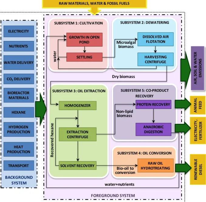
The process was divided into five stages according to the production scheme of the GREET model and the associated sheets of the APD module (Frank et al., 2011a; b):
- S1) cultivation
This stage included the steps of the process that involve the movement of large water volumes, namely the algal growth and the first dewatering step (for the separation of algal biomass from the culture medium and the recycling of the latter to the pond). It was
included water and nutrient consumptions as well as energy requirements of the medium pumping, aeration and the first steps of biomass harvesting. The study focused on the performance of open pond systems, since they are currently the most common and inexpensive large-scale configuration (Davis et al., 2011; Richardson et al., 2012).
- S2) dewatering
According to the baseline harmonized model defined by Davis et al. (2011) a sequential separation based on dissolved air flotation (DAF) followed by a disk-stack centrifuge was considered here.
- S3) oil extraction
Among the different extraction routes available in the APD module (Frank et al., 2011a; b), pressure homogenization and hexane extraction were assumed in this case.
- S4) oil conversion
For the analyzed biorefinery, an hydrotreating process was considered for oil conversion (S4) to obtain renewable diesel, as indicated for the harmonized scenario described by Davis et al. (2012).
- S5) co-product recovery.
The co-product recovery stage (S5) included the separation of protein and fertilizer fractions as well as the AD of remaining biomass to obtain biogas that is then combusted for electricity and heat production.
The complete scheme and the stages within the system boundaries are presented in
Figure 1.
microalgal biodiesel express the results in terms of energy units (e.g. 1 MJ of biodiesel) or mass units (e.g. 1 kg of biodiesel), whereas most techno-economic assessments refer to monetary units per volume of biofuel produced (e.g. $·gal-1 of biodiesel) (Collet et al., 2015; Davis et al., 2014b; Richardson et al., 2012). In the case of integrated economic and environmental assessments, there is no standardized approach to date regarding the selection of a common or two different FUs for economic and environmental indicators respectively. Thus, while some integrated assessments on biodiesel production (from either microalgae or other feedstocks) express each indicator in a specific reference unit (Davis et al., 2014b; Delrue et al., 2012), other authors give a clear definition of a fixed FU used to address both economic and environmental results (Campbell et al., 2011; Wang et al., 2011). In this work, the first approach was selected to allow direct comparisons of each group of indicators with previous studies. Thus, the environmental indicators are calculated for a FU of 1 kg renewable diesel, whereas 1 gal of diesel is selected to refer the economic results in consistency with previous techno-economic
assessments (Davis et al., 2011; 2014b; Richardson et al., 2012; Sun et al., 2011). The second FU (1 gal diesel) is equivalent to 2.95 kg of renewable diesel produced, according to the density specified in GREET model.
The integrated model was validated according to the technological options and the input values from the harmonized scenario. The life cycle inventory for the environmental LCA and the intermediate calculations of the LCC model were determined according to the renewable diesel production pathway from microalgae described by Davis et al. (2012). The information for the selection of values to simulate the stages of cultivation, dewatering and bio-oil extraction was completed with data from the APD module, whereas the conversion of bio-oil to renewable diesel was simulated according to the full GREET model. The costs and other economic parameters were estimated according to the TEA model (Davis et al., 2012; 2014b). The most significant deviation from the original harmonized model was the introduction of a protein recovery step to obtain a fraction with potential uses as animal feed. The main process parameters are listed in
Figure 1. Process chain and system boundaries of the microalgal biorefinery for the
simultaneous production of renewable diesel, animal feed and fertilizer fraction coupled to energy recovery by AD.
A N IM A L FE ED R EN EWA B LE D IE SE L FOREGROUND SYSTEM SUBSYSTEM 2: DEWATERING
SUBSYSTEM 4: OIL CONVERSION
A IR , S O IL & W A TE R EM IS SI O N S BACKGROUND SYSTEM
RAW MATERIALS, WATER & FOSSIL FUELS
NUTRIENTS BIOREACTOR MATERIALS ELECTRICITY WATER DELIVERY CO2DELIVERY RAW OIL HYDROTREATING SUBSYSTEM 3: OIL EXTRACTION
SUBSYSTEM 1: CULTIVATION HOMOGENIZER GROWTH IN OPEN POND SETTLING HEXANE HYDROGEN PRODUCTION HEAT PRODUCTION TRANSPORT DISSOLVED AIR FLOTATION HARVESTING CENTRIFUGE EXTRACTION CENTRIFUGE SOLVENT RECOVERY w a ter Microalgal biomass Dry biomass Bio-oil to conversion SUBSYSTEM 5: CO-PRODUCT RECOVERY PROTEIN RECOVERY ANAEROBIC DIGESTION Non-lipid biomass water+nutrients EL EC TR IC IT Y , FE R TI LI ZE R R eco ve re d he xa ne
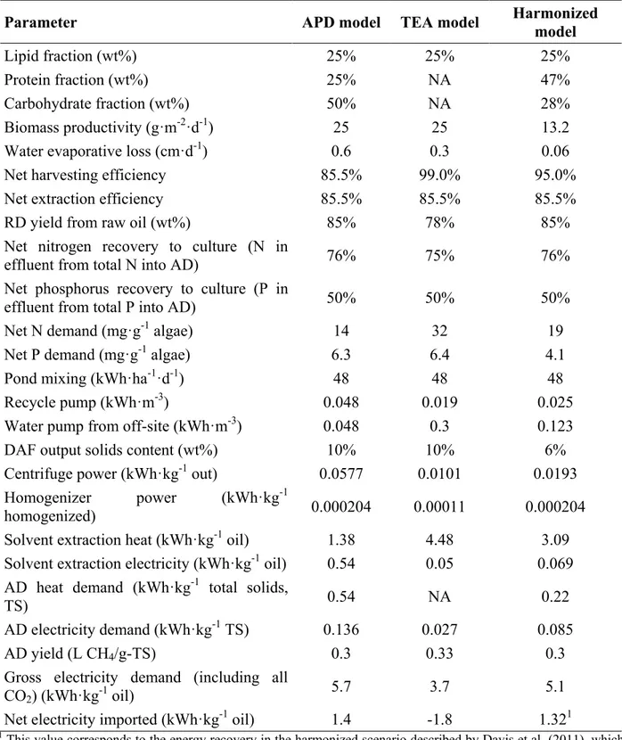
Table 1. Values for the main process parameters according to the original APD and TEA models
and new harmonized parameters
Parameter APD model TEA model Harmonized model
Lipid fraction (wt%) 25% 25% 25%
Protein fraction (wt%) 25% NA 47%
Carbohydrate fraction (wt%) 50% NA 28%
Biomass productivity (g·m-2·d-1) 25 25 13.2
Water evaporative loss (cm·d-1) 0.6 0.3 0.06
Net harvesting efficiency 85.5% 99.0% 95.0%
Net extraction efficiency 85.5% 85.5% 85.5%
RD yield from raw oil (wt%) 85% 78% 85%
Net nitrogen recovery to culture (N in
effluent from total N into AD) 76% 75% 76%
Net phosphorus recovery to culture (P in
effluent from total P into AD) 50% 50% 50%
Net N demand (mg·g-1 algae) 14 32 19
Net P demand (mg·g-1 algae) 6.3 6.4 4.1
Pond mixing (kWh·ha-1·d-1) 48 48 48
Recycle pump (kWh·m-3) 0.048 0.019 0.025
Water pump from off-site (kWh·m-3) 0.048 0.3 0.123
DAF output solids content (wt%) 10% 10% 6%
Centrifuge power (kWh·kg-1 out) 0.0577 0.0101 0.0193 Homogenizer power (kWh·kg-1
homogenized) 0.000204 0.00011 0.000204
Solvent extraction heat (kWh·kg-1 oil) 1.38 4.48 3.09 Solvent extraction electricity (kWh·kg-1 oil) 0.54 0.05 0.069 AD heat demand (kWh·kg-1 total solids,
TS) 0.54 NA 0.22
AD electricity demand (kWh·kg-1 TS) 0.136 0.027 0.085
AD yield (L CH4/g-TS) 0.3 0.33 0.3
Gross electricity demand (including all
CO2) (kWh·kg-1 oil) 5.7 3.7 5.1
Net electricity imported (kWh·kg-1 oil) 1.4 -1.8 1.321
1 This value corresponds to the energy recovery in the harmonized scenario described by Davis et al. (2011), which
considers all non-lipid biomass sent to AD and no protein recovery. In the present study, the protein fraction is first
2.1.1. Environmental LCA
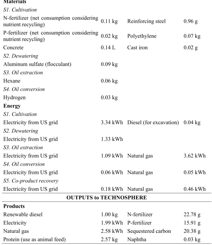
The inventory data for the foreground system included the consumption of nutrients for the culture medium, the chemicals used in the downstream processing (i.e. flocculant for dewatering, hexane for oil extraction and hydrogen for oil hydrotreating) and the energy requirements (electricity and natural gas). As indicated in Davis et al. (2012), the estimation of the materials for the infrastructure (e.g. steel, concrete, polyethylene) was based upon a group of 10 hypothetical facilities of 405 ha each, with 30 years of life span. This group of facilities was equivalent to a total diesel production of approximately 10 million gallons per year, considering 13.2 g·m-2·d-1 biomass productivity and 25% lipid content (harmonized model). Each facility consisted of 100 individual ponds (4 ha each) as well as the equipment for downstream processing. The pond design was based on the technical features proposed by Lundquist et al. (2010).
The background processes (e.g. production of nutrients for cultivation and chemicals for downstream processing, manufacturing process of materials for infrastructure, electricity production) were inventoried according to unit processes from Ecoinvent 2.2 and US LCI databases. All Ecoinvent processes were adjusted to rely on national
average U.S. energy system parameters using the US-EI database (EarthShift, 2009; Frischknecht et al., 2007).
Regarding allocation procedures, renewable diesel (RD) was considered the main product in this study according to the harmonized model used as the baseline scenario. Four additional co-products were obtained in the system: protein fraction with potential applications as animal feed, naphtha separated from renewable diesel in the hydrotreating unit, and fertilizer and energy from the biogas obtained in the AD. CO2 sequestration
potential of cultured algal biomass was also included in the assessment. The environmental benefits of the co-products and CO2 sequestration were computed in the LCA
study as environmental credits by applying a system expansion (avoided burden) approach. For the economic assessment, the market value of the co-products was also accounted for to determine the total revenues of the process.
The global inventory was determined for the selected FU (1 kg renewable diesel) with the integrated simulation model. The inventory data calculated from the simulation of the harmonized scenario are shown in
Table 2. Inventory data for the simulated microalgal biorefinery in the harmonized scenario
(FU=1 kg renewable diesel)
INPUTS from TECHNOSPHERE Materials
S1. Cultivation
N-fertilizer (net consumption considering
nutrient recycling) 0.11 kg Reinforcing steel 0.96 g P-fertilizer (net consumption considering
nutrient recycling) 0.02 kg Polyethylene 0.07 kg
Concrete 0.14 L Cast iron 0.02 g
S2. Dewatering
Aluminum sulfate (flocculant) 0.09 kg
S3. Oil extraction Hexane 0.06 kg S4. Oil conversion Hydrogen 0.03 kg Energy S1. Cultivation
Electricity from US grid 3.34 kWh Diesel (for excavation) 0.04 kg
S2. Dewatering
Electricity from US grid 1.33 kWh
S3. Oil extraction
Electricity from US grid 1.09 kWh Natural gas 3.62 kWh
S4. Oil conversion
Electricity from US grid 0.06 kWh Natural gas 0.05 kWh
S5. Co-product recovery
Electricity from US grid 0.18 kWh Natural gas 0.46 kWh
OUTPUTS to TECHNOSPHERE Products
Renewable diesel 1.00 kg N-fertilizer 22.78 g
Electricity 1.99 kWh P-fertilizer 15.91 g
Natural gas 2.58 kWh Sequestered carbon 20.38 g
The environmental profile was obtained by performing the classification and characterization stages of the LCA methodology (ISO 14040, 2006). In line with the US context of the baseline models, characterization factors from the Tool for the Reduction and Assessment of Chemical and other environmental Impacts (TRACI) model developed by the U.S. Environmental Protection Agency (EPA) were used to evaluate GHG emissions (in CO2 eq),
eutrophication (in N eq), and cumulative energy demand (in MJ). These categories were selected as the most common environmental indicators in LCA studies dealing with environmental aspects of microalgal biofuels (Brentner et al., 2011; Clarens et al., 2010; Montazeri et al., 2016; Soh et al., 2014; Zaimes and Khanna, 2013). The EROI was calculated based on a higher heating value (HHV) of 36 MJ·kg-1 of renewable diesel, obtained from the GREET model.
2.1.2. Economic data
For the economic analysis, a MARR of 10% was assumed and 2011 was selected as the base year, according to previous
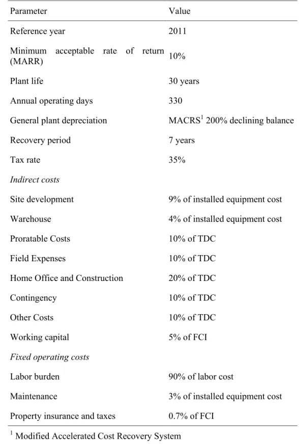
techno-economic assessments (Davis et al., 2014a; b). The equipment costs were estimated from available literature (Benemann and Oswald, 1996; Davis et al., 2012; Lundquist et al., 2010) and updated to 2011-dollars according to the Chemical Engineering Plant Cost Index (CEPCI) from Chemical Engineering magazine (Chemical Engineering, 2012). Overhead cost factors were applied to include other facility costs in the calculation of total direct cost (TDC) and fixed capital investment (FCI). Labor costs were estimated for 2011 according to Davis et al. (2014a). Prices for raw materials and co-products were obtained from the sources indicated in the Supporting Information (Table S6). Prices of chemicals were adjusted to 2011-dollars when required according to the annual average producer price indexes from the U.S. Bureau of Labor Statistics (2017). The main economic parameters (e.g. project lifetime, tax rate, depreciation model) for the first stage of the assessment (single-point analysis for model validation) were estimated from Davis et al. (2014a; 2014b). The considered values are summarized in Table 3.
Table 3. Main economic parameters for model validation (Davis et al., 2014a; 2014b).
Parameter Value
Reference year 2011
Minimum acceptable rate of return
(MARR) 10%
Plant life 30 years
Annual operating days 330
General plant depreciation MACRS1 200% declining balance
Recovery period 7 years
Tax rate 35%
Indirect costs
Site development 9% of installed equipment cost
Warehouse 4% of installed equipment cost
Proratable Costs 10% of TDC
Field Expenses 10% of TDC
Home Office and Construction 20% of TDC
Contingency 10% of TDC
Other Costs 10% of TDC
Working capital 5% of FCI
Fixed operating costs
Labor burden 90% of labor cost
Maintenance 3% of installed equipment cost
Property insurance and taxes 0.7% of FCI
2.2. Sensitivity and uncertainty analysis with @RISK
In the second stage of the integrated assessment, a sensitivity and uncertainty analysis was conducted. Sensitivity and uncertainty analyses are used to evaluate the influence of input variations on a model response (Campolongo et al., 2011; Pianosi et al., 2016; Lacirignola et al., 2017). Uncertainty analysis characterizes the variation of model output, whereas sensitivity analysis determines the relative importance of the variation of each input on the total variation of the output (Campolongo et al., 2011). This variation includes the uncertainty due inability of the model to describe the real system and the inherent variability of model inputs (Sills et al., 2013; Lacirignola et al., 2017).
Variability and uncertainty are often measured in a localized region of the input parameter space, and the potential changes are quantified separately for each parameter, assuming no changes in the other inputs (Campolongo et al., 2011; Sills et al., 2013; Tu et al., 2017). These methods fail at considering variations over the whole range of values of each parameter and detecting interactions that can only be found when changing parameters simultaneously. To overcome these drawbacks, the use of probability-based methods to propagate the uncertainty of all input parameters throughout the model is currently increasing (Campolongo et al., 2011; Iooss and
al., 2017). Among the tools to apply these methods, the Monte Carlo simulation serves to generate a large number of scenarios using sets of input data that are randomly sampled from each parameter’s individual probability distribution function (PDF). It can be used to analyze statistical uncertainty and allows the evaluation of single uncertain parameters separately or of a set of multiple parameters jointly. However, without careful separation of the model into independent parameters, the random generation of values for the parameters may conduct to inconsistent scenarios, especially when working with complex multi-variable models. Therefore, correlations among input data need to be considered and validity checks may be required in these systems (Iooss and Lemaître, 2015; Pianosi et al., 2016; Sills et al., 2013).
In this case, after model validation, Monte Carlo simulation was selected to analyze the effect of the uncertainty and variability of input parameters on the economic and environmental results, based on PDFs for the relevant inputs. To do so, the licensed Excel add-in @RISK from Palisade Corporation (Ithaca, NY) was used to generate the scenarios and identify the possible correlations between the results (Palisade Corp., 2017).
Firstly, the uncertain input parameters were defined by substituting the baseline values previously specified in the corresponding cells by PDFs. Then, the output parameters
mathematical relationships between them and the input parameters according to Excel formulas. Once the input and output parameters as well as the corresponding PDFs were defined, the number of iterations and sampling methods were specified and the simulation was executed. The simulation results provided by @RISK included the PDF of each output parameter, the list of individual scenarios evaluated during the simulation (with values for all input and output parameters), detailed statistical information for each input and output (e.g. mean value, minimum and maximum values, standard deviation, variance, percentiles) and graphical representations of the behavior of the different parameters and the correlations between parameters.
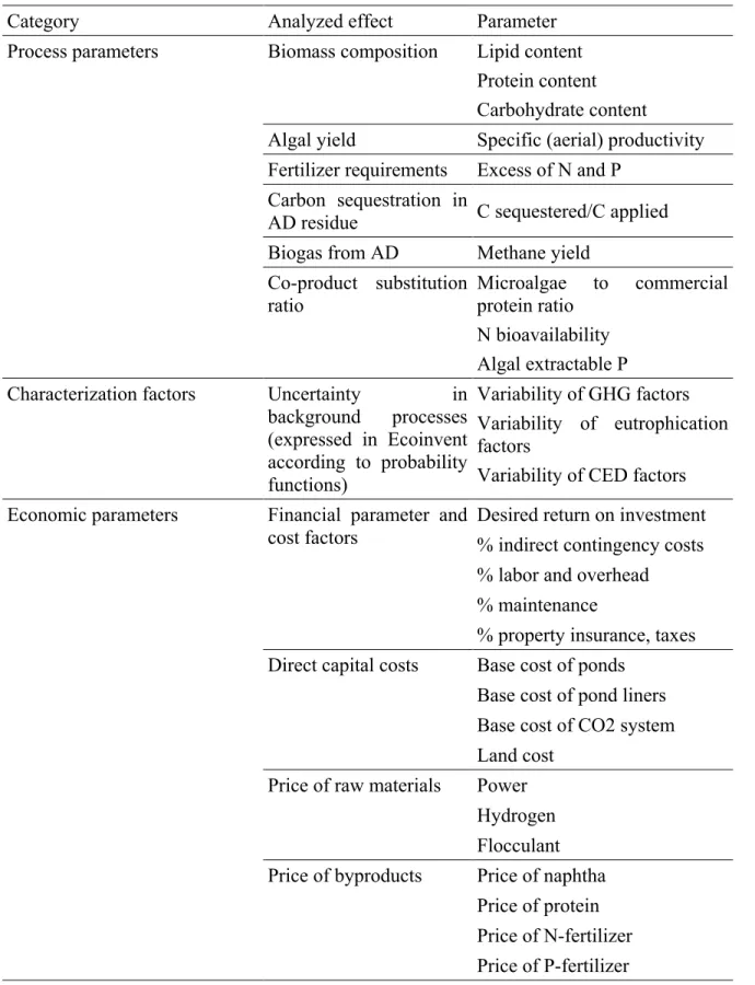
The input parameters were classified in three groups: i) process parameters, ii) characterization factors and iii) economic parameters. The specific parameters included in each group are listed in Table 4. The PDFs reflected the range of possible values for each input parameter and the probability of each value. They were obtained either from literature sources or from experimental data fitting. The estimated PDFs and the corresponding data sources are indicated in the Supplementary Information.
Table S2 presents the data for process parameters. The distribution functions for biomass composition and productivity were
obtained with @RISK Distribution Fitting tool from experimental data for microalgae
Chlorella sorokiniana, Nannocloropsis
oculata and Neochloris oleabundans grown at
lab-scale under nitrogen-deplete conditions using different cultivation periods. Due to the large variability of growth parameters depending on species and conditions, uniform distributions gave the best fit. Other parameters including nutrient excess, co-product substitution ratio (which measures the equivalency between the obtained co-product and the similar product for which the environmental credits are calculated) and AD yield were estimated from the literature assuming triangular distributions (Bryant et al., 2012; Mulbry et al., 2005; Sills et al., 2013).
In the case of characterization factors, the distribution function indicated in Tables S3, S4 and S5 for each environmental indicator and Ecoinvent unit process was calculated by using the Monte Carlo Analysis tool available in SimaPro, and fitted to a distribution using @RISK Distribution Fitting tool (Goedkoop et al., 2013; Palisade Corp., 2017). The distributions reflect the uncertainty established by the authors of the ecoinvent datasets, associated with data quality criteria. Three types of distributions gave the best fitting results: normal distribution, lognormal distribution and log-logistic distribution.
Table 4. Classification of the variable parameters included in the uncertainty analysis
Category Analyzed effect Parameter
Process parameters Biomass composition Lipid content Protein content Carbohydrate content
Algal yield Specific (aerial) productivity Fertilizer requirements Excess of N and P
Carbon sequestration in
AD residue C sequestered/C applied Biogas from AD Methane yield
Co-product substitution
ratio Microalgae to commercial protein ratio N bioavailability
Algal extractable P Characterization factors Uncertainty in
background processes (expressed in Ecoinvent according to probability functions) Variability of GHG factors Variability of eutrophication factors
Variability of CED factors Economic parameters Financial parameter and
cost factors
Desired return on investment % indirect contingency costs % labor and overhead % maintenance
% property insurance, taxes Direct capital costs Base cost of ponds
Base cost of pond liners Base cost of CO2 system Land cost
Price of raw materials Power Hydrogen Flocculant Price of byproducts Price of naphtha
Price of protein Price of N-fertilizer
Regarding the economic parameters (Table S6), the MARR and cost factors were adjusted to triangular distributions, considering the different assumptions from previous assessments related to algae (Davis et al., 2011; 2012; 2014a; 2014b; Lundquist et al., 2010) and other biomass sources (Humbird et al., 2011). The direct capital cost of ponds, pond liners and CO2 system were
introduced as normal distributions. The mean (µ) was equal to the initial value used for model validation and standard deviation σ was set as 10% of the mean. Land cost function was obtained by adjusting average U.S. farm values per state (USDA, 2014) with @RISK Distribution Fitting tool. The price of electricity and flocculant were introduced as triangular distributions according to the variability in the period 2007-2014. Data for electricity were obtained from EIA (2017) whereas the initial price of flocculant was adjusted with the price index for chemicals (U.S. Bureau of Labor Statistics, 2017). The prices of hydrogen (raw material), naphtha and fertilizers (co-products) were also fitted to triangular distributions according to the minimum and maximum values from the sensitivity analysis by Davis et al. (2014a). The price of protein used for animal feed was estimated according to a triangular function with the same range as soybean meal for the period between January 2011 and January 2012 (IndexMundi, 2017). The different quality of the algal protein was already taken into account by the process parameter
―co-3. Results and discussion
3.1. Environmental results for harmonized scenario
Before conducting the uncertainty assessment, the model was validated with the parameters of the harmonized scenario. According to TRACI model, a value of 2.46 kg CO2 eq·kg-1 was calculated for GHG
emissions. Eutrophication potential was -0.02 kg N eq·kg-1 and CED was 21.51 MJ·kg-1. The characterization results for the harmonized scenario are consistent with previous results in the literature. Although most of these studies refer to biodiesel rather than renewable diesel, the difference associated with the conversion stage has been found to be sufficiently limited so as to allow straightforward comparisons for the two products. Thus, Zaimes and Khanna (2013) found that the choice of fuel conversion to obtain either biodiesel or renewable diesel had a minimal impact on life cycle results, compared to variations in biomass production pathways.
The calculated GHG emissions are in the range of 0.5-4.5 kg CO2 eq·kg-1 of algal
diesel reported for best scenarios in previous works (Campbell et al., 2011; Davis et al., 2014b; Montazeri et al., 2016; Tu et al., 2017; Zaimes and Khanna, 2013). For eutrophication potential, as explained below in more detail, the co-product credits totally compensate the environmental burdens and lead to a negative impact. This means that the protein and fertilizer obtained in the process
routes with higher environmental burdens, and therefore avoid these impacts. The results for eutrophication show a better profile than previous findings, although the favorable performance of algae compared to other feedstocks (i.e. terrestrial crops) was already pointed out in the literature with low reported values, usually below 0.20 kg N eq·kg-1 of diesel (Brentner et al., 2011; Clarens et al., 2010; Montazeri et al., 2016). The energy demand indicated in Table 5 can be expressed as EROI by dividing the heating potential of 1 kg renewable diesel by the calculated CED. Assuming a standard HHV of 37 MJ·kg-1 (Montazeri et al., 2016), the harmonized scenario leads to a favorable EROI=1.72 MJ produced·MJ-1 consumed. This result is in the range of previous LCA studies (Clarens et al., 2010; Collet et al., 2014, Montazeri et al., 2016; Sills et al., 2013; Tu et al., 2017; Zaimes and Khanna, 2013), including the EROI values between 1-4 MJ produced·MJ-1 consumed.
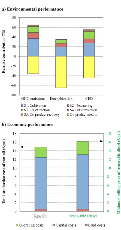
The relative contributions per stage are depicted in Figure 2a. Among the production stages, cultivation has the largest effect, regardless of the considered impact category. Its contribution exceeds 50% of the total environmental impact for all the indicators. Most of the impact of the cultivation stage (between 70% and 90%) is due to the electricity consumption for media circulation and, to a lesser extent, for CO2 supply. This
finding is in agreement with the results from previous LCAs (Collet et al., 2014; Davis et
the culture media has contributions between 3% and 11% depending on the impact category, whereas the infrastructure is responsible for 4% to 17% of the environmental impact. Dewatering and oil extraction have similar contributions to GHG emissions (20% each approximately), mainly linked to their energy requirements. Oil extraction is the second stage (after cultivation) affecting CED due to both electricity requirements of the pressure homogenizer and the natural gas consumed for heating in the solvent extraction. For eutrophication, dewatering has a higher impact than oil extraction due to the higher electricity consumption, which is linked to NOx emissions in power plants.
The three categories show high reductions of impact related to the environmental benefits of co-products. In the case of eutrophication, the credits from the production of protein fraction alone are higher than the total impact of the microalgae production stages. For this reason, the environmental impact has a negative value, meaning that the obtained co-products allow avoiding the production of alternative substances with higher impacts than the whole process analyzed here. The environmental benefits of co-products for the reduction of GHG emissions are equivalent to 55% of the total impacts, whereas the credits for CED represent 81% of the total demand throughout the production stages. These results are comparable to the findings of
The final GHG emissions are therefore 55% lower than the total emissions that the process would have if no co-product was obtained,
whereas the energy balance is 80% lower than the CED of the same process with no co-products.
Figure 2. Environmental and economic results for harmonized scenario: a) Relative
contributions of microalgal production of renewable diesel, protein fraction and fertilizer coupled to energy recovery by AD per stage and b) Breakdown of oil production costs (blue axis) and diesel minimum selling price (red axis), considering 10% MARR and 2011 as the base year.
3.2. Economic results for harmonized scenario
The economic results were calculated assuming a 10% MARR and using 2011 as the base year, according to the approach of Davis et al. (2014b). For the operational parameters of the harmonized scenario, a total production cost of $14.91 gal-1 of raw oil is obtained when the production of renewable biodiesel is coupled to the production of protein and fertilizer fractions and the remaining biomass is subjected to an AD process to recover energy in the form of biogas (Figure 2b). This production cost corresponds to a minimum selling price of $16.18 gal-1 of renewable diesel.
The obtained values are significantly higher than the results reported by Davis et al. (2011) for open ponds, although they are below the values given for tubular PBR in the same assessment. The main reason for the worse economic performance of the harmonized scenario is the lower biomass productivity. Thus, the productivity considered by Davis et al. (2011) corresponds to the value of 25 g·m-2·d-2 indicated in Table
1 for the original TEA model. As explained
by Davis et al. (2012), the application of the RA model (mentioned in Section 2) resulted in an estimate of the mean annual biomass productivity of 13.2 g·m-2·d-1, which was significantly lower than the value considered in the original APD and TEA models. Thus, Davis et al. (2012) indicate that the application of the new scenario led to
remarkably higher costs and emissions than the previous estimates.
When comparing the results of the scheme analyzed in this paper with the values from Davis et al. (2014b), the minimum selling price is close to the range of $10-15 gal-1 for
biomass productivities between 10-14 g·m-2·d-1. The slightly higher value
found for this study is principally linked to the different approach considered for the oil conversion stage. The scenario evaluated by Davis et al. (2014b) includes a hydrothermal liquefaction (HTL) step instead of the pathway considered in the current study. Other factors are related to the fluctuations in prices and economic parameters. Since these fluctuations are inherent of the system and cannot be avoided, the following uncertainty assessment will complete the information and give a wider view of the possible economic performances of the process.
According to Figure 2b, the production costs for microalgal biodiesel are mainly associated with the capital costs. Thus, nearly 80% of the total cost is due to the capital investment required for the establishment of the facility, the construction of the production systems and other related costs. Operating costs involve less than 20% of the total, whereas land costs are below 5%. The low contribution of land to the final cost reflects one of the main advantages of microalgae: the possibility to cultivate algal biomass in marginal and non-competitive land with low value. Regarding operating costs, about 40%
and insurance, while electricity is responsible for 16%, and nutrients, waste management and labor costs are in the range of 10-15% each. The sum of other operating costs is below 10% of the total.
3.3. Sensitivity and uncertainty analysis with @RISK tool
In this stage, the relevant uncertain parameters were defined as @RISK inputs according to the probability distribution functions listed in the Supplementary Information (Tables S1 to S6). The four performance indicators were defined as outputs together with the parameter ―others‖. This parameter refers to the percentage of remaining biomass (mostly the mineral fraction of the biomass) after subtracting lipid, protein and carbohydrate content. It was included as an output in the simulation to ensure (by applying an @RISK filter to the parameter) that the sum of lipid, protein and carbohydrate fractions was below 100% in all the simulated scenarios. Once the inputs and outputs were defined, the Monte Carlo simulation was run for 5000 iterations.
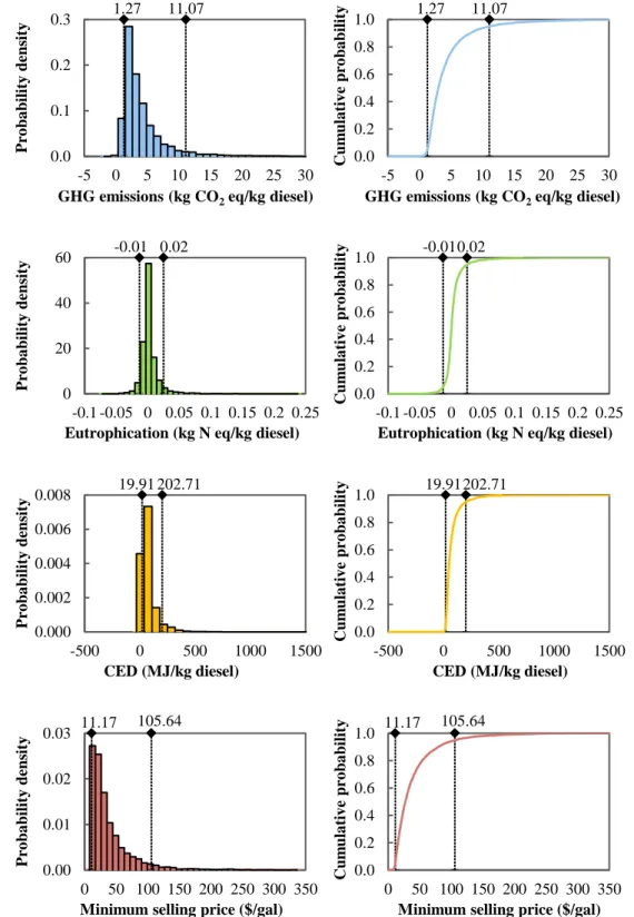
3.3.1. Total variability and probability distribution functions for output parameters
The main statistical results are summarized in Table 5. The ranges of possible values for the measured economic and environmental indicators are depicted in Figure 3, which shows the probability density function and cumulative distribution function for each parameter. According to the results, GHG emissions in 90% of the evaluated scenarios
-1
renewable diesel, whereas eutrophication varies from a negative impact of -0.013 kg N eq·kg-1 diesel to 0.025 kg N eq·kg-1 diesel and the energy demand is between 19 and 203 MJ·kg-1. Although the highest values for GHG emissions and CED show a less favorable environmental profile than the best cases reported in the literature, the ranges are consistent with common average values (Campbell et al., 2011; Clarens et al., 2010; Montazeri et al., 2016; Sills et al., 2013; Tu et al., 2017; Zaimes and Khanna, 2013). Thus, there is a 65% probability of GHG emissions in the range of 0.5-4.5 kg CO2 eq·kg-1 of
diesel from previous LCA studies indicated in Section 3.1 (Campbell et al., 2011; Davis et al., 2014b; Montazeri et al., 2016; Soh et al., 2014; Tu et al., 2017; Zaimes and Khanna, 2013). In the case of eutrophication, the results show the benefits related to the integration of co-products in the biorefinery scheme, especially associated with the credits from the protein fraction and, to a lesser extent, from the recovered fertilizer. The range of CED values is consistent with the EROI results of different LCA studies reported by Sills et al. (2013). Thus, the results reflect a 98% probability of EROI values between 0.1 and 4 MJ produced·MJ-1 consumed. In particular, 71% of cases may have an unfavorable CED above 37 MJ·kg-1 diesel meaning that the EROI<1 (for a HHV of 37 MJ·kg-1 diesel) and hence, the required energy exceeds the produced energy. Favorable CED values leading to EROI>1
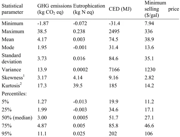
Table 5. Statistical parameters of the probability distributions for the four evaluated indicators Statistical parameter GHG emissions (kg CO2 eq) Eutrophication (kg N eq) CED (MJ) Minimum selling price ($/gal) Minimum -1.87 -0.072 -31.4 7.94 Maximum 38.5 0.238 2495 336 Mean 4.17 0.003 74.5 38.9 Mode 1.95 -0.001 31.4 13.6 Standard deviation 3.73 0.016 84.6 35.1 Variance 13.9 0.0002 7166 1230 Skewness1 3.17 4.14 9.16 2.82 Kurtosis2 17.3 39.5 185 14.2 Percentiles: 5% 1.27 -0.013 19.9 11.2 25% 1.99 -0.003 34.6 17.1 50% (median) 3.00 0.0005 51.7 27.1 75% 4.87 0.005 85.8 46.6 95% 11.1 0.025 202 106
1 Measure of the symmetry of the probability distribution. For symmetrical distributions,
skewness=0.
2 Measure of the shape of the probability distribution. High values of kurtosis involve
distributions with sharp peaks and thick tails. Regarding the economic performance, the obtained diesel should be sold at a minimum price between $11-106 gal-1 with a probability of 90%. This range is wider than the estimates between $0.9-43 gal-1 from previous assessments (Lundquist et al., 2010; Richardson et al., 2012; Sun et al., 2011). The variability of the results is linked to the large number of variable process and economic parameters that are considered in the current study, as well as the wide range of variation
for each parameter. In contrast, most of the previous techno-economic assessments considered a single case study or a limited number of changes. Despite the high variability of the indicator, the probability of maintaining a minimum selling price below $28 gal-1 exceeds 50%, whereas only 25% of the situations would result in prices above $46 gal-1. This finding is consistent with the aforementioned range from the literature.
Figure 3. Probability density function and cumulative distribution function for economic and
environmental indicators, including percentiles 5% and 95%.
1.27 11.07 0.0 0.1 0.2 0.3 -5 0 5 10 15 20 25 30 P ro ba bil it y dens it y
GHG emissions (kg CO2eq/kg diesel)
1.27 11.07 0.0 0.2 0.4 0.6 0.8 1.0 -5 0 5 10 15 20 25 30 Cum ula tiv e pro ba bil it y
GHG emissions (kg CO2eq/kg diesel)
-0.01 0.02 0 20 40 60 -0.1 -0.05 0 0.05 0.1 0.15 0.2 0.25 P ro ba bil it y dens it y
Eutrophication (kg N eq/kg diesel)
-0.010.02 0.0 0.2 0.4 0.6 0.8 1.0 -0.1 -0.05 0 0.05 0.1 0.15 0.2 0.25 Cum ula tiv e pro ba bil it y
Eutrophication (kg N eq/kg diesel)
19.91 202.71 0.000 0.002 0.004 0.006 0.008 -500 0 500 1000 1500 P ro ba bil it y dens it y CED (MJ/kg diesel) 19.91202.71 0.0 0.2 0.4 0.6 0.8 1.0 -500 0 500 1000 1500 Cu m u la tiv e p ro b a b il ity CED (MJ/kg diesel) 11.17 105.64 0.00 0.01 0.02 0.03 0 50 100 150 200 250 300 350 P ro ba bil it y dens it y
Minimum selling price ($/gal)
11.17 105.64 0.0 0.2 0.4 0.6 0.8 1.0 0 50 100 150 200 250 300 350 Cu m u la tiv e p ro b a b il ity
3.3.2. Correlations between the economic and environmental indicators
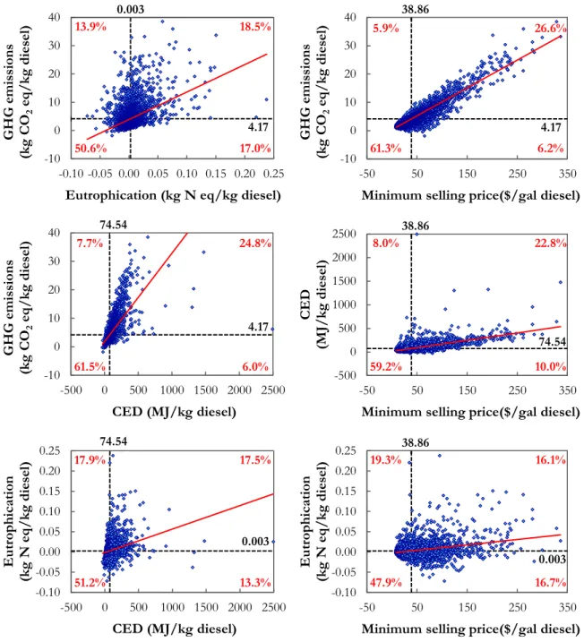
The scatter plots showing the variability of the results from the Monte Carlo simulation for each pair of indicators are presented in
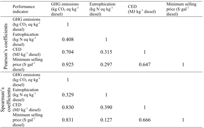
Figure 4. Pearson’s and Spearman’s
correlation coefficients are shown in Table 6. Pearson’s correlation coefficient measures the strength of the linear relationship between two variables. Spearman’s coefficient is a nonparametric measure of interdependence between variables that are not necessarily linear but can be related to each other by a monotone function (Pianosi et al., 2016).
According to Pearson’s coefficients, GHG emissions and minimum selling price have the strongest positive linear relationship. This connection can be partially attributed to the GHG emissions derived from the use of electricity, which also involve significant operating costs. However, the Pearson’s coefficients that reflect the environmental performance of the system in terms of CED with respect to the minimum selling price and the coefficient that links GHG emissions with CED have lower values. This suggests that CED is affected by a variable parameter that has a lesser influence in GHG emissions and minimum selling price. The deviation may be linked to the co-product credits, which involve remarkable reductions of environmental impact. In particular, the credits associated with the protein fraction involve a reduction between 0.5% and 42% of the CED of the production stages, whereas the
15% for GHG emissions and generates less than 11% of annual revenues. Eutrophication shows weak linear correlation with the other three indicators. The values indicate the lack of a linear relationship of eutrophication with the other measured indexes. This finding may be due, to a large extent, to the higher influence of co-product credits in eutrophication results compared to their effect on the other categories.
Despite the different type of mathematical relationship measured by Spearman’s correlation coefficient, the results show common trends compared to Pearson’s coefficients. Thus, the association of GHG emissions with minimum selling price has again the highest correlation coefficient. In this case, the coefficient that describes the relationship between GHG emissions and CED is remarkably higher than Pearson’s value and only 0.2% lower than the coefficient describing GHG variability with respect to the economic indicator. This finding reflects the clear interdependence of the two parameters, despite the non-linearity of the relationship. Spearman’s correlation coefficients for eutrophication also show the low connection of this parameter with the other indicators.
Figure 4 also indicates the probability of
combinations in each quadrant. Regardless of the pair of performance indicators, most of the simulated scenarios are included in the third quadrant. The results indicate a high probability of achieving production scenarios
eq·kg-1 diesel, eutrophication potential below 0.003 kg N eq·kg-1 diesel, CED lower than 74
MJ·kg-1 diesel and a minimum selling price below $39 gal-1.
Figure 4. Correlations between the analyzed performance indicators
74.54 4.17 -10 0 10 20 30 40 -500 0 500 1000 1500 2000 2500 G HG emi ss ions (kg CO 2 eq /kg dies el ) CED (MJ/kg diesel) 0.003 4.17 -10 0 10 20 30 40 -0.10 -0.05 0.00 0.05 0.10 0.15 0.20 0.25 G H G emis si ons (kg CO 2 eq /kg dies el )
Eutrophication (kg N eq/kg diesel)
13.9% 18.5% 50.6% 17.0% 38.86 4.17 -10 0 10 20 30 40 -50 50 150 250 350 G HG emi ss ions (kg CO 2 eq /kg dies el )
Minimum selling price($/gal diesel)
5.9% 26.6% 61.3% 6.2% 7.7% 24.8% 61.5% 6.0% 38.86 74.54 -500 0 500 1000 1500 2000 2500 -50 50 150 250 350 CED (MJ/kg dies el )
Minimum selling price($/gal diesel)
8.0% 22.8% 59.2% 10.0% 74.54 0.003 -0.10 -0.05 0.00 0.05 0.10 0.15 0.20 0.25 -500 0 500 1000 1500 2000 2500 Eu tr ophicatio n (kg N e q/ kg d ies el ) CED (MJ/kg diesel) 17.9% 17.5% 51.2% 13.3% 38.86 0.003 -0.10 -0.05 0.00 0.05 0.10 0.15 0.20 0.25 -50 50 150 250 350 Eu tr ophicatio n (kg N e q/ kg d ies el )
Minimum selling price($/gal diesel)
19.3% 16.1%
Table 6. Statistical parameters of the probability distributions for the four evaluated indicators Performance indicator GHG emissions (kg CO2 eq·kg-1 diesel) Eutrophication (kg N eq·kg-1 diesel) CED (MJ·kg-1 diesel) Minimum selling price ($·gal-1 diesel) Pear son’ s co ef ficie nts GHG emissions (kg CO2 eq·kg-1 diesel) 1 Eutrophication (kg N eq·kg-1 diesel) 0.408 1 CED (MJ·kg-1 diesel) 0.704 0.315 1 Minimum selling price ($·gal-1 diesel) 0.925 0.297 0.647 1 Spear ma n’s coef fici ent s GHG emissions (kg CO2 eq·kg-1 diesel) 1 Eutrophication (kg N eq·kg-1 diesel) 0.329 1 CED (MJ·kg-1 diesel) 0.830 0.390 1 Minimum selling price ($·gal-1 diesel) 0.831 0.127 0.666 1
3.3.3. Effect of individual parameter uncertainty on the economic and environmental results
The Monte Carlo simulation allowed the evaluation of the possible scenarios and the likelihood of each economic and environmental performance. The analysis considered a wide range of variable parameters simultaneously. However, the model may be more sensitive to changes in certain parameters than to others. To analyze the different effects of process parameters, characterization factors and economic parameters, three additional simulations were conducted by varying one group of parameters separately. The results are
Process parameters are the main cause of uncertainty for all the analyzed indicators, whereas characterization factors have a moderate contribution to the variability of eutrophication potential and CED. Economic parameters are a limited source of uncertainty for the minimum selling price. Other types of uncertainties could be considered in future analyses. In terms of process parameters, additional categorical parameters could be integrated in the model to evaluate the effect of the selection of technological alternatives. In the case of methodological uncertainties, which are included here only in terms of variable characterization factors, other influencing aspects could be considered, such
economic allocation, or the uncertainties linked to geographical, temporal and technological representativeness of background data. These uncertainties have not been included in the current study to avoid an excessive number of parameters (with a limited individual influence on the variability of the results) that could hinder the interpretability of the results.
In the Monte Carlo simulation for the analysis of process parameters, GHG emissions ranged between 1.30 and 10.90 kg CO2 eq·kg-1 renewable diesel with a
probability of 90%. This interval is consistent with the global variability of the indicator presented in Figure 3. Characterization factors had a very limited effect and involve changes lower than 10% compared to the median.
Eutrophication potential varies from -0.009 to 0.016 kg N eq·kg-1 diesel in 90% of the scenarios, when considering the uncertainty of process parameters. This interval represents 67% of the global range of values presented in Figure 3. Although the variation with respect to the characterization factors is
more limited, they involve significant changes in the indicator, which has a 90% probability of values between -0.005 to 0.010 kg N eq·kg
-1 diesel.
CED also has a remarkable level of uncertainty associated with the variability of process parameters. Thus, 90% confidence interval includes values from 25 to 188 MJ·kg-1 diesel, which correspond to an uncertain EROI between 0.19 and 1.40 MJ produced per MJ consumed. The results point out the need of a careful optimization of the operating conditions to obtain a favorable energy balance. The characterization factors have a lower influence in the indicator and lead to variations from 25 to 74 MJ·MJ-1.
As in the case of GHG emissions, most of the uncertainty of the minimum selling price is due to the uncertainty of the process parameters. Thus, the diesel price may range between $10 and $98 gal-1 with a probability of 90% depending on the process parameters, while this interval is limited to $20-26 gal-1 when the effect of economic assumptions is analyzed separately.
Figure 5. Boxplot of results for performance indicators grouped by type of input parameter
(representing percentiles 5%, 25%, 50%, 75% and 95%).
0 2 4 6 8 10 12
Characterization factors
Process parameters
GHG emissions (kg CO2eq/kg diesel)
-0.015 -0.01 -0.005 0 0.005 0.01 0.015 0.02
Characterization factors
Process parameters
Eutrophication (kg N eq/kg diesel)
0 20 40 60 80 100 120 140 160 180 200
Characterization factors
Process parameters
CED (MJ eq/kg diesel)
0 20 40 60 80 100 120
Economic parameters
Process parameters
Since process parameters were identified as the main cause of uncertainty for all the analyzed indicators, the individual effect of each variable included in this category is presented in Figure 6. According to the results, biomass productivity is a key factor affecting all the environmental indicators. Thus, the uncertainty of this variable leads to the widest interval of likely values in the three categories. Productivity also has a remarkable influence in the minimum selling price, although the variability of this economic indicator is higher with respect to the lipid content. The possible values of the lipid fraction result in a wide range of prices from $12 gal-1 up to $78 gal-1, while the indicator has a 95% probability of values below $52 gal-1 for the complete range of productivities. The high variability of GHG emissions and minimum selling price related to lipid content may be one of the reasons of the stronger mathematical relationship between those indicators compared to the correlations with CED. In addition, parameters related to the protein recovery (i.e. protein content and microalgal to commercial substitution ratio) have a higher secondary contribution in the case of CED than for the other two indicators. This suggests that environmental credits associated with the protein may involve higher reductions of
impact for CED than for GHG. The eutrophication potential is also affected by the uncertainty of protein content. Methane yield has a moderate contribution to the uncertainty of the environmental indicators, but it barely affects the economic performance. These results indicate the environmental benefits of energy recovery, which are more limited in economic terms due to the low relative contribution of operating costs to the total costs of the facility (already shown in Figure
2b). Other process parameters included in the
uncertainty assessment such as carbohydrate content, nutrient excess or nitrogen and phosphorus bioavailability have a very limited effect on all the performance indicators.
The main findings of this step of the analysis confirm the key role of productivity and lipid content in the global performance of microalgal systems, already highlighted in previous studies (Davis et al., 2014b; Sills et al., 2013). Conversely, the uncertainty related to other process parameters, characterization factors and especially economic parameters has a limited influence on the environmental and economic performance. In addition, the results show moderate benefits of co-product credits, which are especially significant in certain environmental categories such as eutrophication and energy balance.
Figure 6. Individual effect of process parameters on a) GHG emissions, b) eutrophication, c)
CED and d) minimum selling price (representing percentiles 5%, 25%, 50%, 75% and 95%).
0 20 40 60 80 100
Minimum selling price ($/gal diesel) 0 20 40 60 80 100 120 Protein substitution ratio P bioavailability (%) N bioavailability (%) CH yield (L CH /g VS) Carbon sequestration (g C seq./g C applied) Nutrient excess (%) Carbohydrate (wt%) Protein (wt%) Lipid (wt%) Biomass productivity (g/m /d)
CED (MJ eq/kg diesel)
2
4 4
-0.010 -0.005 0.000 0.005 0.010 0.015
Eutrophication (kg N eq/kg diesel)
0 2 4 6 8 Protein substitution ratio P bioavailability (%) N bioavailability (%) CH yield (L CH /g VS) Carbon sequestration (g C seq./g C applied) Nutrient excess (%) Carbohydrate (wt%) Protein (wt%) Lipid (wt%) Biomass productivity (g/m /d)
GHG emissions (kg CO2eq/kg diesel) 2