Static interpretation of higher-order modules in Futhark: functional GPU programming in the large

HAL Id: hal-01883524

https://hal.inria.fr/hal-01883524

Submitted on 2 Oct 2018

HAL is a multi-disciplinary open access

archive for the deposit and dissemination of

sci-entific research documents, whether they are

pub-lished or not. The documents may come from

teaching and research institutions in France or

abroad, or from public or private research centers.

L’archive ouverte pluridisciplinaire HAL, est

destinée au dépôt et à la diffusion de documents

scientifiques de niveau recherche, publiés ou non,

émanant des établissements d’enseignement et de

recherche français ou étrangers, des laboratoires

publics ou privés.

Futhark: functional GPU programming in the large

Martin Elsman, Troels Henriksen, Danil Annenkov, Cosmin Oancea

To cite this version:

Martin Elsman, Troels Henriksen, Danil Annenkov, Cosmin Oancea. Static interpretation of

higher-order modules in Futhark: functional GPU programming in the large. Proceedings of the ACM on

Programming Languages, ACM, 2018, 2 (ICFP), pp.97:1–97:30. �10.1145/3236792�. �hal-01883524�

Static Interpretation of Higher-Order Modules in Futhark:

Functional GPU Programming in the Large

MARTIN ELSMAN,

TROELS HENRIKSEN,

DANIL ANNENKOV

,

COSMIN E. OANCEA,

We present a higher-order module system for the purely functional data-parallel array language Futhark. The module language has the property that it is completely eliminated at compile time, yet it serves as a powerful tool for organizing libraries and complete programs. The presentation includes a static and a dynamic semantics for the language in terms of, respectively, a static type system and a provably terminating elaboration of terms into terms of an underlying target language. The development is formalised in Coq using a novel encoding of semantic objects based on products, sets, and finite maps. The module language features a unified treatment of module type abstraction and core language polymorphism and is rich enough for expressing practical forms of module composition.

CCS Concepts: • Software and its engineering → Abstraction, modeling and modularity; Parallel programming languages; Functional languages; Modules / packages; Seman-tics;

Additional Key Words and Phrases: modules, GPGPU, functional languages, compilers ACM Reference Format:

Martin Elsman, Troels Henriksen, Danil Annenkov, and Cosmin E. Oancea. 2018. Static Interpreta-tion of Higher-Order Modules in Futhark: FuncInterpreta-tional GPU Programming in the Large. Proc. ACM

Program. Lang. 2, ICFP, Article 97 (September 2018),31pages.https://doi.org/10.1145/3236792

1 INTRODUCTION

Programming massively parallel hardware is increasingly becoming a central aspect of developing computational software kernels. Research in developing programming abstraction mechanisms for effectively utilizing massively parallel hardware has resulted in a number of available tools, ranging from low-level programming models, such as CUDA and OpenCL, over domain-specific languages and libraries, such as Accelerate [Chakravarty et al. 2011;

McDonell et al. 2013], Obsidian [Claessen et al. 2012; Svensson 2011], Lift [Steuwer et al.

∗_{Work done while at the University of Copenhagen.}

Authors’ addresses: Martin Elsman, Department of Computer Science, University of Copenhagen, hagen, Denmark, mael@di.ku.dk; Troels Henriksen, Department of Computer Science, University of Copen-hagen, CopenCopen-hagen, Denmark, athas@di.ku.dk; Danil Annenkov, GALLINETTE Research team, Inria, Nantes, France, danil.annenkov@inria.fr; Cosmin E. Oancea, Department of Computer Science, University of Copenhagen, Copenhagen, Denmark, coancea@di.ku.dk.

Permission to make digital or hard copies of all or part of this work for personal or classroom use is granted without fee provided that copies are not made or distributed for profit or commercial advantage and that copies bear this notice and the full citation on the first page. Copyrights for components of this work owned by others than the author(s) must be honored. Abstracting with credit is permitted. To copy otherwise, or republish, to post on servers or to redistribute to lists, requires prior specific permission and/or a fee. Request permissions from permissions@acm.org.

© 2018 Copyright held by the owner/author(s). Publication rights licensed to ACM. 2475-1421/2018/9-ART97

2015,2017], and CUBLAS, to full programming languages, such as SaC [Guo et al. 2011] and Futhark [Henriksen et al. 2014;Henriksen and Oancea 2014;Henriksen et al. 2017].

With software components that utilise massively parallel hardware getting larger and more complicated, an increasing need emerges in this area for good software structuring mechanisms and high reusability of developed software components. In the last decades, a number of abstraction mechanisms have been introduced that allow programmers to reason at a high level about the composition of developed software components. Such mechanisms include object-oriented class-based programming mechanisms, type class structuring mechanisms, as found in Haskell [Wadler and Blott 1989], module-languages as found in Standard ML [Milner et al. 1997] and OCaml [Leroy 1995], and extensions [Rossberg and Dreyer 2013] and combinations [Dreyer et al. 2007;White et al. 2015] thereof.

A common issue with the work on modules, and abstraction mechanisms in general, is that the mechanisms seldom give guarantees about their overhead. Often, the mechanisms introduce runtime overhead in terms of, for instance, dynamic method invocation, or packages (e.g., dictionaries or modules) being passed around at runtime. At best, an optimizing compiler can eliminate much of this overhead statically, but the interaction between the core language and the language for programming in the large is often subtle and without paying attention to the interaction mechanisms, it will be difficult for a compiler to provide guarantees that refactoring for increasing modularity will not affect performance.

One promising technique for solving some of these issues is the work on embedded domain-specific languages (EDSLs), which provide a structuring mechanism based on host language features for structuring and composing components. Examples of such approaches to orchestrate programming for massively parallel hardware include Accelerate, Obsidian, and Firepile [Nystrom et al. 2011], which are libraries, written in Haskell and Scala, for synthesizing code for running on GPGPUs. However, designing a well-working EDSL is not a trivial task as the developer needs to work hard, for instance to avoid unintended code duplication [Mainland and Morrisett 2010]. Another issue with EDSLs is that they can be difficult to incorporate in code generation pipelines as the language cannot necessarily be understood in isolation from its host-language, which may cause both practical problems and reasoning problems with respect to guaranteeing correctness of a compilation pipeline. In this paper, we introduce the notion of higher-order static interpretation. The work is based on earlier work on static interpretation for Standard ML [Elsman 1999], which provides a technique for complete static elimination of modules, including first-order modules (called functors in Standard ML). The technique is similar to how C++ templates are eliminated at compile time with the difference that modules are type checked before they are compiled. The present paper extends the previous work to higher-order modules. We demonstrate the usefulness of the added functionality and argue for the need for higher-order modules and type abstraction. The module language is implemented on top of the monomorphic, first-order functional data-parallel language Futhark, which features a number of polymorphic second-order array combinators (SOACs) with parallel semantics, such as map, reduce,

scan, and filter. The Futhark core language makes it possible to write data-parallel kernels

that are often competitive with hand-written CUDA or OpenCL applications [Andreetta et al. 2016; Henriksen et al. 2016b, 2017; Larsen and Henriksen 2017]. We show that the practical implications of the module language give rise to highly reusable components, which, for instance, form the grounds of a Basis Library for Futhark.

Although the basic module language that we present is both elegant and simple, it features a number of derived forms, which makes the language practical while keeping the technical details minimal. Special derived forms allow programmers to declare certain

kinds of polymorphic higher-order functions and types. The declarations are turned into parameterised modules, which are then instantiated at the module level for each use.

An essential property of static interpretation of higher-order modules is that it is strongly normalizing, which is based on a logical-relation argument, similar to an argument for strong-normalisation of the simply-typed lambda-calculus [Tait 1967]. The important properties of the module language (e.g., normalisation of static interpretation) has been proven in Coq and both the Futhark compiler, featuring the full module language, and the Coq implementation are available online.

In summary, we claim the following novel contributions:

(1) We show how the concept of static interpretation can be extended to higher-order modules and present an implementation as part of a compiler for Futhark.

(2) We demonstrate the usefulness of a higher-order module system for GPU program-ming by presenting a number of modularised Futhark examples and by arguing (and demonstrating) that the modularisation has no influence on performance.

(3) Using a novel adaptation of a logical-relation argument, we show that static interpre-tation terminates and that target and source programs are typed consistently. (4) We provide a formal development in Coq, which uses a novel encoding of semantic

objects for modules based on products, sets, and finite maps. The encoding closely resembles the paper formalisation and the implementation for Futhark.

The paper is organised as follows. In the next section, we introduce the higher-order module language and present a motivating example demonstrating the use of higher-order modules in Futhark. In Section3, we give an overview of how static interpretation turns higher-order modules into monomorphic core language Futhark code. In Section4, we present the static semantics for the module language and show how the module language interacts with the core language. Section 5presents the technicalities of static interpretation and Section6presents the main technical result, namely that static interpretation terminates and that the resulting program, from a type perspective, is consistent with the source program, which may possibly contain declarations and applications of higher-order modules. In Section 7, we briefly discuss the type inference algorithm. In Section 8, we present a number of derived forms for allowing programmers to use traditional syntax for polymorphic functions and function application for generating parameterised code at the module level and for instantiating this code also at the module level. In Section9, we discuss the Coq development and in Section10, we discuss the application of the module language in the concrete setting of the Futhark compiler. We present a few larger examples of Futhark modules and demonstrate that, in practice, the module language is a useful technology for improving code reuse and code abstraction and that it introduces no overhead with respect to performance of the generated code. In Section11and Section12, we discuss related work and conclude.

2 THE MODULE LANGUAGE

The module language can be considered parameterised over a core language, which, for the purpose of the presentation, is a simple functional language. In the practical implementation, the core language is a full-fledged programming language for data-parallel programming featuring a number of second-order polymorphic array combinators (SOACs) with parallel semantics but with no support for user-defined polymorphic higher-order functions.

For the core language considered here, we assume denumerably infinite sets of type identifiers (tid), value identifiers (vid), and module identifiers (mid). For each of the above

mty ::= {spec } | mtid

| mid : mty₁→ mty₂ | mty with longtid = ty spec ::= val vid : ty

| type tid

| module mid : mty

| include mty

| spec₁ spec₂ | 𝜖

mexp ::= {mdec }

| mid | mexp . mid | 𝜆mid : mty → mexp | longmid (mexp) mdec ::= dec

| type tid = ty

| module mid = mexp

| module type mtid = mty

| open mexp

| mdec1 mdec2 | 𝜖 Fig. 1. Grammar for the module language excluding derived forms.

identifier sets 𝑋, we define the associated set of long identifiers Long𝑋, inductively with 𝑋 as the base set and mid.long𝑥 as the inductive case with long𝑥 ∈ Long𝑋 and mid being a module identifier. For the module language, we also assume a denumerably infinite set of module type identifiers (mtid). Long identifiers, such as 𝑥.𝑦.𝑧, allow users to use traditional dot-notation for accessing components deep within modules and the separation of identifier classes makes it clear in what syntactic category an identifier belongs.

The simple core language is defined by notions of type expressions (ty), core language expressions (exp), and core language declarations (dec):

ty ::= longtid | ty1→ ty2

exp ::= longvid | 𝜆vid → exp | exp1 exp2 | exp : ty

dec ::= val vid = exp

The core language can be understood entirely in isolation from the module language except that long identifiers may be used to access values and types in modules. As will become apparent in the typing rules for the core language, the construct 𝜆vid → exp binds vid in exp and the declaration of a value identifier in a val-declaration allows for other declarations to depend on it. For simplicity, composition of core language constructs are handled entirely by the module language and so is the possibility for declaring types. An important aspect here is that the dependency structure between declarations is not allowed to be cyclic.

The grammar for the module language is given in Figure 1. The module language is separated into a language for specifying module types (mty) and a language for declaring modules (mdec). The language for module types is a two-level language with sub-languages for specifying module components and for expressing module types. Similarly, the language for declaring (i.e., defining) modules is a two-level language for declaring module components and for expressing module manipulations. At the toplevel, a program is a module declaration, possibly consisting of a sequence of module declarations where later declarations may depend on earlier declarations. To resolve ambiguities, parentheses are allowed around module type expressions and around module expressions. As will become apparent from the typing rules, in declarations of the form mdec1mdec2, identifiers declared by mdec1are considered bound in mdec2 (similar considerations hold for composing specifications and programs).

Without lack of generality, a number of additional constructs are supported by considering them derived forms, following [Milner et al. 1997] and [Rossberg et al. 2014]. Such derived forms include constructs for local module bindings, direct application of a module expression

to another module expression, constructs for opaque matching (in Standard ML terms), and support for type abbreviations in module type specifications:

module 𝐹 ( 𝑋 : mty ) = mexp mdec=⇒ module 𝐹 = 𝜆𝑋 : mty → mexp (1)

local mdec in mexp mdec=⇒ open let mdec in mexp (2)

let mdec in mexp mexp=⇒ {mdec module 𝑋 = mexp } . 𝑋 (3) mexp₁(mexp₂ ) mexp=⇒ let module 𝐹 = mexp₁ in 𝐹 (mexp₂) (4) mexp : mty mexp=⇒ (𝜆𝑋 : mty → 𝑋) (mexp) (5)

module 𝑋 : mty = mexp mdec=⇒ module 𝑋 = mexp : mty (6)

module 𝐹 ( 𝑋 : mty₀ ): mty = mexp mdec=⇒ module 𝐹 ( 𝑋 : mty₀ )= mexp : mty(7) type tid = ty =⇒spec include ({ type tid } with tid = ty)(8)

Although the derived form of Equation5, for matching a module expression to a module type expression, allows us to simplify the semantic treatment of the module language, we shall later present a specialised typing rule specifying how a module expression mexp is classified by a given module type expression mty under some environment. Type abbreviations in module type specifications are also considered a derived form (Equation8) using an include construct and a with-constrained module type expression, which in itself is arguably more expressive than a type abbreviation, as it resembles a substitution and allows for reuse of module types. Another possible derived form introduces a construct for modeling the semantics of OCaml’s open construct (not shown here), which opens a module in a local scope contrary to the semantics of open defined here, which resembles the semantics of

open in Standard ML.

As described in more detail in Section 8, certain kinds of polymorphic higher-order functions and polymorphic types, as known from traditional higher-order polymorphic languages such as Standard ML, OCaml, and Haskell, can also be introduced as derived forms together with derived forms for instantiating such declared higher-order modules. By introducing derived forms only at the module level, we can be sure that all modules are indeed eliminated entirely at compile time.

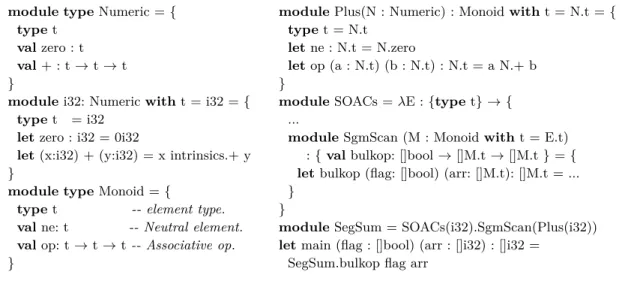
We conclude this section by discussing a practical example, shown in Figure2, in which the module language is used to extend, at library level, the set of SOACs supported in Futhark. Notice that the syntax for types is extended to also support array types, which take the form []𝜏 , for some 𝜏 , which may possibly also be an array type. Here, the aim is to implement segmented scan based on the natively supported scan bulk-parallel operator,1

which is applied in the main function. The implementation starts by declaring a Numeric module type that exports a numeric type t, a zero element (of type t), and various numeric operations such as addition. A possible implementation is given by module i32, which instantiates t to 32-bit integers.

Next, the Monoid module type is declared to export a type t, together with a binary associative operator op with neutral element ne:t. A potential implementation for Monoid

1 _{scan ⊙ e [a}

1, . . ., a𝑛] results in the array [e⊙a1,...,e⊙a1 ⊙ . . . ⊙a𝑛], where ⊙ is a binary

associative operator with neutral element e. Segmented scan [Blelloch 1989,1990] receives as extra argument a flag array, which records the start of a new segment with a one and zero otherwise, and results in a (flat) array obtained by applying scan on each segment of the input array.

module type Numeric = { type t

val zero : t val + : t → t → t }

module i32: Numeric with t = i32 = { type t = i32

let zero : i32 = 0i32

let (x:i32) + (y:i32) = x intrinsics.+ y }

module type Monoid = {

type t -- element type.

val ne: t -- Neutral element.

val op: t → t → t -- Associative op. }

module Plus(N : Numeric) : Monoid with t = N.t = { type t = N.t

let ne : N.t = N.zero

let op (a : N.t) (b : N.t) : N.t = a N.+ b }

module SOACs = 𝜆E : {type t} → { ...

module SgmScan (M : Monoid with t = E.t) : { val bulkop: []bool → []M.t → []M.t } = { let bulkop (flag: []bool) (arr: []M.t): []M.t = ... }

}

module SegSum = SOACs(i32).SgmScan(Plus(i32)) let main (flag : []bool) (arr : []i32) : []i32 =

SegSum.bulkop flag arr

Fig. 2. Implementing segmented scan based on scan at library level in Futhark.

module type MT = {

module F: (X:{ val b:i32 } → { val f:i32→i32 }) }

module H = 𝜆(M:MT) → M.F { let b = 8 } module Main =

H ( { module F =

𝜆(X:{ val b:i32 }) → { let f(x:i32) = X.b+x }

})

let main (a:i32) : i32 = Main.f a

(a) Example source program.

val b = 8

val f = 𝜆(x:i32) → b + x

val main = 𝜆(a:i32) → f a

(b) Target language code.

Fig. 3. A (contrived) example demonstrating static interpretation in action. The program on the left is turned into the three snippets of declarations on the right.

is the parameterised module Plus, which receives a module parameter N implementing Numericand instantiates Monoid’s t, zero and op with N.t, N.zero and N.+, respec-tively. Finally, new SOACs are derived from the ones natively supported by Futhark in the parameterised module SOACs, which receives as parameter a monoid E corresponding to the array element type, and declares an inner parameterised module for each new SOAC. For example, SgmScan takes as parameter a monoid-implementing module M, and implements the segmented-scan operator bulkop based on Futhark’s scan (not shown). Function main computes a segmented scan with the plus operator on a (segmented) array of 32-bit integers.

3 EXECUTIVE SUMMARY

For the purpose of demonstrating static interpretation in action, consider the (contrived) example Futhark program in Figure3a. Compared to the motivating example in Section2, the program here makes no use of derived forms and it therefore serves well as a running example demonstrating the technique. The program declares a module type MT and a

higher-order module H, which is applied to a module containing a parameterised module F. The result of the module application is a module containing a function f of type i32 → i32. The contained function is called in the main function with the input to the program.

The static semantics of the language, which we shall later define in terms of a set of elaboration rules, provides evidence that the code in Figure3ais well-typed with the intended guarantee that the program can be executed without dynamic type errors occurring.

Static interpretation for the example in Figure 3a partially evaluates the program to achieve the three code snippets shown in Figure3b. Each of the three code snippets contains monomorphic target code, which can be composed, analysed, and compiled without any module language considerations. This feature provides the target language implementor with the essential meta-level abstraction property that the module language features are orthogonal to the domain of the source language. In other words, the target language implementor need not worry that the added modularity constructs will have any influence on composing the generated code. This property is essential for targeting data-parallel architectures, such as GPUs, but may also be essential for a variety of other domain specific languages, including languages for financial contracts [Peyton Jones et al. 2000], probabilistic programming, hardware design, signal processing, and formal reasoning.

At the technical side, static interpretation takes care of renaming identifiers properly to resolve scope-issues. In Section6, we demonstrate that if the source language is well-typed then (1) static interpretation will generate target language code and (2) the generated target language code will be consistent with the source language code with respect to the types of declared identifiers. An essential aspect of the approach is that the generation of target code is shown to be terminating using a logical-relations argument, which is properly formalised and backed up by a proof in Coq. For limiting the scope of the presentation, we shall not here provide the reader with a direct dynamic semantics for the module language. Instead, the dynamic semantics for the language can be understood as the composition of static interpretation and the dynamic semantics of the target language. Providing a direct dynamic semantics for the module language, along the lines of the dynamic semantics of

Milner et al.[1997], would be straightforward and would resemble closely the rules for static interpretation.

In what follows, we develop the precise formalism that makes static interpretation possible, including a proper treatment of abstract types at the module language level.

4 STATIC SEMANTICS

The static semantics that we present here elaborates well-typed syntactic constructs into so-called semantic objects, which are based on well-established mathematical constructs such as products, finite maps, and sets. This style of elaboration approach resembles closely the style of elaboration set forward byMilner et al. [1997], although modified to use universal and existential quantification for treating certain objects equal up-to 𝛼-renaming, as set forward byRusso[1999] andElsman[1999].

For the static semantics, we assume a denumerably infinite set TSet of type variables (t). A semantic type (or simply a type), ranged over by 𝜏 , takes the form:

𝜏 ::= 𝑡 | 𝜏1→ 𝜏2

Types relate straightforwardly to syntactic types with the difference that syntactic types contain type identifiers and semantic types contain type variables. This difference is essential in that it enables the support for type parameterisation and type abstraction.

𝐸 = (TE , VE , ME , 𝐺) ∈ Env = TEnv × VEnv × MEnv × MTEnv ME ∈ MEnv = Mid→ Modfin

𝑀 ∈ Mod = Env ∪ FunSig

𝐹 = ∀𝑇.(𝐸, Σ) ∈ FunSig = Fin(TSet) × Env × MTy Σ = ∃𝑇.𝑀 ∈ MTy = Fin(TSet) × Mod

𝐺 ∈ MTEnv = MTid→ MTyfin

Fig. 4. Module language semantic objects. Parameterised module types (𝐹 ) and module types (Σ) are parameterised over finite sets of type variables (written Fin(TSet)), ranged over by 𝑇 .

At the core level, a value environment (VE ) maps value identifiers (vid) to types and a type environment (TE ) maps type identifiers (tid) to types.

The module language semantic objects are shown in Figure 4. The semantic objects constitute a number of mutually dependent inductive definitions. An environment (𝐸) is a quadruple (TE , VE , ME , 𝐺) of a type environment TE , a variable environment VE , a module environment (ME ), which maps module identifiers to modules, and a module type environment (𝐺), which maps module type identifiers to module types. A module is either an environment 𝐸, representing a non-parameterised module, or a parameterised module type 𝐹 , which is an object ∀𝑇.(𝐸, Σ), for which the type variables in 𝑇 are considered bound. A module type (Σ) is a pair, written ∃𝑇.𝑀 , of a set of type variables 𝑇 and a module 𝑀 . In a module type ∃𝑇.𝑀 , type variables in 𝑇 are considered bound and we consider module types identical up-to renaming of bound variables and removal of type variables that do not appear in 𝑀 . When 𝑇 is empty, we often write 𝑀 instead of ∃∅.𝑀 . We consider module function types ∀𝑇.(𝐸, Σ) identical up-to renaming of bound type variables and removal of type variables in 𝑇 that do not occur free in (𝐸, Σ).

When 𝑋 is some tuple and when 𝑥 is some identifier, we shall often write 𝑋(𝑥) for the result of looking up 𝑥 in the appropriate projected finite map in 𝑋. Moreover, when long𝑥 is some long identifier, we write 𝑋(long𝑥) to denote the lookup in 𝑋, possibly inductively through module environments.

When 𝑋 and 𝑌 are finite maps, the modification of 𝑋 by 𝑌 , written 𝑋 + 𝑌 , is the map with Dom(𝑋 + 𝑌 ) = Dom 𝑋 ∪ Dom 𝑌 and values

(𝑋 + 𝑌 )(𝑥) = {︂

𝑌 (𝑥) if 𝑥 ∈ Dom 𝑌 𝑋(𝑥) otherwise

The notion of modification is extended point-wise to tuples, as are operations such as Dom, ∩, and ∪. A finite map 𝑋 extends another finite map 𝑋′, written 𝑋 ⊒ 𝑋′, if Dom 𝑋 ⊇ Dom 𝑋′ and 𝑋(𝑥) = 𝑋′(𝑥) for all 𝑥 ∈ Dom 𝑋′.

Given a particular kind of environment, such as a module environment ME , we shall often be implicit about its injection ({}, {}, ME , {}) into environments of type Env. Moreover, given an identifier, such as tid, its class specifies exactly that, given some type 𝜏 , {tid ↦→ 𝜏 } denotes a type environment of type TE , which again, by the above convention, can be injected implicitly into an environment of type Env.

As an example, if t is a type identifier, a and b are value identifiers, and A is a module identifier, we can write {t ↦→ 𝑡} + {A ↦→ {a ↦→ 𝑡}} for specifying the environment 𝐸 = ({t ↦→ 𝑡}, {}, {A ↦→ 𝐸′}, {}), where 𝐸′ _{= ({}, {a ↦→ 𝑡}, {}, {}) and where 𝐸 ⊒ {t ↦→ 𝑡}. Moreover,} looking up the long identifier A.a in 𝐸, written 𝐸(A.a), yields 𝑡.

𝐸𝑃 𝑟𝑔 = ( {}, {main ↦→ (i32 → i32)}, ME𝑃 𝑟𝑔, {MT ↦→ Σ𝑀 𝑇} ) where

ME𝑃 𝑟𝑔 = {Main ↦→ M𝑓, H ↦→ ∀∅.( ({}, {}, {F ↦→ Σ𝐹}, {}), ∃∅.M𝑓 )}

Σ𝑀 𝑇 = ∃∅.({}, {}, {F ↦→ Σ𝐹}, {})

Σ𝐹 = ∀∅.( ({}, {b ↦→ i32}, {}, {}), ∃∅.M𝑓)

M𝑓 = ( {}, {f ↦→ (i32 → i32)}, {}, {} )

Fig. 5. The semantic objects at outermost (program) level for the code example in Figure3.

Figure5shows the outer-level environment for the code example in Figure3, which are obtained by applying the elaboration (typing) rules, which are presented in the remainder of this section.

4.1 Enrichment

Enrichment specifies that an environment, in an inductive sense, has the same or more ele-ments than another environment. Enrichment is mutually and inductively defined on module environments, modules, and environments. The concept is central to the understanding of parameterised module application and matching. An environment 𝐸′ = (TE′, VE′, ME′, 𝐺′) enriches another environment 𝐸 = (TE , VE , ME , {}), written 𝐸′ ≻ 𝐸, if VE′ _{⊒ VE ,}

TE′ ⊒ TE , and ME′ _{≻ ME . A module environment ME}′ _{enriches another module} envi-ronment ME , written ME′ ≻ ME , if Dom ME′ _{⊇ Dom ME and ME}′_{(mid) ≻ ME (mid)} for each mid ∈ Dom ME . A module 𝑀′ = 𝐸′ enriches another module 𝑀 = 𝐸, written 𝑀′ ≻ 𝑀 , if 𝐸′ _{≻ 𝐸. Moreover, a module 𝑀}′ _{= ∀𝑇}′_.(𝐸′_{, Σ}′_{) enriches another module}

𝑀 = ∀𝑇.(𝐸, Σ), written 𝑀′≻ 𝑀 , if 𝑇′_{= 𝑇 and 𝐸 ≻ 𝐸}′ _{and Σ}′ _{≻ Σ.}

Notice that enrichment for parameterised modules is contravariant in parameter environ-ments. Notice also the special treatment of module type environenviron-ments. Because a module type cannot specify bindings of module types (such a possibility creates a number of problems that are complementary to static interpretation), we can safely require that when 𝐸′≻ 𝐸, the module type environment in 𝐸 is empty. A simpler approach was chosen than a more rigid semantic object structure that would capture precisely the non-supportedness of module type bindings inside modules.

4.2 Instantiation

Another central concept for understanding parameterised module application and module matching is the notion of instantiation, which is used for capturing that a particular module is a concrete instance of a generic module type. Instantiation is based on the notion of a substitution (𝑆), which maps type variables to types. The result of applying a substitution 𝑆 to an object 𝑋, written 𝑆(𝑋), is first to extend the substitution to be the identity outside its domain and then simultaneously substitute each type variable 𝑡 in 𝑋 with 𝑆(𝑡), after appropriately renaming bound type variables in 𝑋. The support of a substitution 𝑆, written Supp 𝑆, is the set of elements 𝑡 for which 𝑆(𝑡) ̸= 𝑡.

Formally, then, an object 𝐴 instantiates another object 𝐵, written 𝐴 ≤ 𝐵, if the judgement can be derived according to the following rules:

𝐸 ≤ 𝐸′ Dom(ME ) = Dom(ME′)

∀mid ∈ Dom(ME ), ME (mid) ≤ ME′_(mid) (TE , VE , ME , 𝐺) ≤ (TE , VE , ME′, 𝐺)

𝐹 ≤ 𝐹′ (𝐸, Σ) ≤ ∀𝑇′.(𝐸′, Σ′) 𝑇 ∩ tvs(∀𝑇′.(𝐸′, Σ′)) = ∅ ∀𝑇.(𝐸, Σ) ≤ ∀𝑇′_.(𝐸′_{, Σ}′₎

Type Expressions. 𝐸 ⊢ ty : 𝜏 𝐸(longtid) = 𝜏 𝐸 ⊢ longtid : 𝜏 (9) 𝐸 ⊢ ty_𝑖: 𝜏𝑖 𝑖 = [1, 2] 𝐸 ⊢ ty₁→ ty₂: 𝜏1→ 𝜏2 (10)

Core Language Expressions. 𝐸 ⊢ exp : 𝜏

𝐸(longvid) = 𝜏 𝐸 ⊢ longvid : 𝜏 (11) 𝐸 ⊢ exp : 𝜏 𝐸 ⊢ ty : 𝜏 𝐸 ⊢ exp : ty : 𝜏 (12) 𝐸 + {vid ↦→ 𝜏 } ⊢ exp : 𝜏′ 𝐸 ⊢ 𝜆vid → exp : 𝜏 → 𝜏′ (13) 𝐸 ⊢ exp₁: 𝜏 → 𝜏′ 𝐸 ⊢ exp₂: 𝜏 𝐸 ⊢ exp₁exp₂: 𝜏′ (14) Fig. 6. Elaboration rules for the core language. The rules are straightforward but illustrate the interaction between the module language and the core language through the concept of long identifiers.

𝐸 ≤ Σ Supp(𝑆) ⊆ 𝑇 𝐸 ≤ 𝑆(𝐸′) 𝐸 ≤ ∃𝑇.𝐸′ Σ ≤ Σ′ 𝑇 ∩ tvs(∃𝑇′.𝐸′) = ∅ 𝐸 ≤ ∃𝑇′.𝐸′ ∃𝑇.𝐸 ≤ ∃𝑇′.𝐸′ (𝐸, Σ) ≤ ∀𝑇′.(𝐸′, Σ′) Supp(𝑆) ⊆ 𝑇 𝑆(𝐸′) ≤ 𝐸 Σ ≤ 𝑆(Σ′) (𝐸, Σ) ≤ ∀𝑇′.(𝐸′, Σ′) Notice the contravariance in the rule for instantiating a parameterised module type and that instantiation is applied inductively in the rules, which differs from how instantiation is defined in the case for first-order modules [Milner et al. 1997]. For instance, with this revised instantiation relation, given that {t ↦→ 𝜏 } represents an environment mapping a type constructor to a type 𝜏 , a concrete parameterised module type ∀∅.({}, {t ↦→ i32}) instantiates the more abstract parameterised module type ∀∅.({}, ∃{𝑡}.{t ↦→ 𝑡}).

The notion of matching combines the notions of enrichment and instantiation. An environ-ment 𝐸 matches a module type Σ if there exists another environenviron-ment 𝐸′ such that 𝐸 ≻ 𝐸′ and 𝐸′ _{≤ Σ. Matching is central in the elaboration rule for applications of parameterised} modules and to the notions of encapsulation and abstraction, in general.

4.3 Elaboration

Elaboration of the module language is based on elaboration rules for the core language, which are straightforward and presented in Figure6. The rules are split into rules for type expressions and rules for value expressions and allow for inferences of the forms 𝐸 ⊢ ty : 𝜏 and 𝐸 ⊢ exp : 𝜏 , which are read “under assumptions 𝐸, the type expression ty (or value expression exp) is elaborated to have type 𝜏 ”. Notice how the core language interacts with the module language through the use of long identifiers in Rule9and Rule11.

Elaboration of module types and specifications is defined as a mutual inductive relation allowing inferences among sentences of the forms 𝐸 ⊢ mty : Σ and 𝐸 ⊢ spec : ∃𝑇.𝐸′. The rules are presented in Figure 7. There is a subtle difference between module type expressions (mty) and specifications (spec). Whereas module type expressions may elaborate to parameterised module types, specifications only elaborate to non-parameterised module types, which may, however, contain parameterised modules inside. Thus, in Rule 22, we require that the included module is a non-parameterised module type.

The most interesting of the rules are Rule16, the rule for with-types, and Rule18, the rule for expressing parameterised modules as dependent products [Harper and Lillibridge 1994].

Module Types. 𝐸 ⊢ mty : Σ 𝐸(mtid) = Σ

𝐸 ⊢ mtid : Σ (15)

𝐸 ⊢ ty : 𝜏 𝐸′(longtid) = 𝑡 𝑡 ∈ 𝑇 𝐸 ⊢ mty : ∃𝑇.𝐸′ Σ = ∃(𝑇 ∖ {𝑡}).(𝐸′[𝜏 /𝑡])

𝐸 ⊢ mty with longtid = ty : Σ (16)

𝐸 ⊢ spec : Σ

𝐸 ⊢ { spec } : Σ (17)

𝐸 ⊢ mty₁: ∃𝑇.𝐸′ 𝑇 ∩ (tvs(𝐸) ∪ 𝑇′) = ∅ 𝐸 + {mid ↦→ 𝐸′} ⊢ mty₂: ∃𝑇′.𝑀

𝐸 ⊢ mid : mty₁→ mty₂: ∀𝑇.(𝐸′, ∃𝑇′.𝑀 ) (18)

Module Specifications. 𝐸 ⊢ spec : ∃𝑇.𝐸′

𝐸 ⊢ type tid : ∃{t}.{tid ↦→ t} (19)

𝐸 ⊢ ty : 𝜏

𝐸 ⊢ val vid : ty : ∃∅.{vid ↦→ 𝜏 } (20) 𝐸 ⊢ mty : ∃𝑇.𝑀

𝐸 ⊢ module mid : mty : ∃𝑇.{mid ↦→ 𝑀 } (21)

𝐸 ⊢ mty : ∃𝑇.𝐸′ 𝐸 ⊢ include mty : ∃𝑇.𝐸′ (22) 𝐸 ⊢ spec₁: ∃𝑇1.𝐸1 𝐸 + 𝐸1⊢ spec2: ∃𝑇2.𝐸2 𝑇1∩ (tvs(𝐸) ∪ 𝑇2) = ∅ Dom 𝐸1∩ Dom 𝐸2= ∅ 𝐸 ⊢ spec₁ spec₂: ∃(𝑇1∪ 𝑇2).(𝐸1+ 𝐸2) (23) 𝐸 ⊢ 𝜖 : ∃∅.{} (24) Fig. 7. Elaboration rules for module types and module specifications. This sub-language does not directly depend on the rules for module expressions and module declaration.

The rule for with-types (also called where-types in Standard ML) allows a programmer to refine a module type to a more concrete module type. The rule for expressing parameterised module types allow a programmer to express dependencies between the parameter module and the result module by referring to the module identifier associated with the parameter. As an example, consider the module type expression

X:{ type t val a : t } → { val b : X.t }

This module type expression elaborates, using, among others, Rule (16), to the module type ∀{𝑡}.({t ↦→ 𝑡, a ↦→ 𝑡}, ∃∅.{b ↦→ 𝑡})

An essential aspect of the semantic technique is that of requiring, for instance, that the sets 𝑇1and 𝑇2in Rule (23) are disjoint. This property can always be satisfied by 𝛼-renaming, which is applied often (and in the Coq implementation, explicitly) when proving properties.

4.4 Elaboration Rules for Module Expressions and Module Declarations

The elaboration rules for module language expressions and declarations are given in Figure8 and allow inferences among sentences of the forms 𝐸 ⊢ mdec : Σ and 𝐸 ⊢ mexp : ∃𝑇.𝐸. The rules make use of the previously introduced rules for module type expressions and core language declarations and types. Similarly to the elaboration difference between module type expressions and specifications, module expressions elaborate to general module types ∃𝑇.𝑀 , whereas module declarations elaborate to non-parameterised module types ∃𝑇.𝐸.

The by far most complicated rule is Rule (29), the rule for application of a parameterised module. The rule looks up a parameterised module type ∀𝑇0.(𝐸0, Σ0) for the long module

Module Expressions. 𝐸 ⊢ mexp : Σ 𝐸 ⊢ mdec : Σ 𝐸 ⊢ { mdec } : Σ (25) 𝐸 ⊢ mexp : ∃𝑇.𝐸′ 𝐸′(mid) = 𝐸′′ 𝐸 ⊢ mexp . mid : ∃𝑇.𝐸′′ (26) 𝐸(mid) = 𝐸′ 𝐸 ⊢ mid : ∃∅.𝐸′ (27) 𝐸 ⊢ mty : ∃𝑇.𝐸′ 𝐸 + {mid ↦→ 𝐸′} ⊢ mexp : Σ 𝑇 ∩ tvs(𝐸) = ∅ 𝐹 = ∀𝑇.(𝐸′, Σ)

𝐸 ⊢ 𝜆mid : mty → mexp : ∃∅.𝐹 (28)

𝐸 ⊢ mexp : ∃𝑇.𝐸′ 𝑇 ∩ 𝑇′ = ∅ (𝐸′′, ∃𝑇′.𝐸′′′) ≤ 𝐸(longmid) 𝐸′≻ 𝐸′′ _{(𝑇 ∪ 𝑇}′_{) ∩ tvs(𝐸) = ∅}

𝐸 ⊢ longmid ( mexp ) : ∃(𝑇 ∪ 𝑇′).𝐸′′′ (29)

Module Declarations. 𝐸 ⊢ mdec : ∃𝑇.𝐸′

mdec = dec 𝐸 ⊢ dec : 𝐸′ 𝐸 ⊢ mdec : ∃∅.𝐸′ (30)

𝐸 ⊢ ty : 𝜏

𝐸 ⊢ type tid = ty : ∃∅.{tid ↦→ 𝜏 } (31) 𝐸 ⊢ mexp : ∃𝑇.𝑀

𝐸 ⊢ module mid = mexp : ∃𝑇.{mid ↦→ 𝑀 } (32)

𝐸 ⊢ mexp : Σ

𝐸 ⊢ open mexp : Σ (33) 𝐸 ⊢ mty : Σ

𝐸 ⊢ module type mtid = mty : ∃∅.{mtid ↦→ Σ} (34) 𝐸 ⊢ 𝜖 : ∃∅.{} (35) 𝑇1∩ (tvs(𝐸) ∪ 𝑇2) = ∅ 𝐸 ⊢ mdec1: ∃𝑇1.𝐸1 𝐸 + 𝐸1⊢ mdec2: ∃𝑇2.𝐸2

𝐸 ⊢ mdec1mdec2: ∃(𝑇1∪ 𝑇2).(𝐸1+ 𝐸2)

(36) Fig. 8. Elaboration rules for module language expressions and declarations.

identifier in the environment and seeks to match the parameter module type ∃𝑇0.𝐸0 against a cut-down version (according to the enrichment relation) of the module type resulting from elaborating the argument module expression. The result of elaborating the application is the result module type, perhaps with additional abstract type variables stemming from elaborating the argument module expression. The need for also quantify over the type set 𝑇 in the result module type comes from the desire to prove a property that if 𝐸 ⊢ mexp : ∃𝑇.𝐸′ then tvs(𝐸′_{) ⊆ tvs(𝐸) ∪ 𝑇 . The remainder of the rules cover the other constructs of the} language, which include Rule 26, for module projection, and Rule 28, for parameterised modules. In the rule for parameterised modules, the side condition 𝑇 ∩ tvs(𝐸) = ∅ expresses that 𝑇 should be chosen sufficiently fresh. Notice in particular that, due to 𝛼-renaming, the judgement 𝐸 ⊢ mty : ∃𝑇.𝐸′does not by itself entail this property. Another important aspect to notice is that both Rule26and Rule36are implicit about removal of bound type variables that do not occur under the binder, as objects are considered identical up-to removal of superfluous type variables. In Rule36, for instance, due to shadowing of identifiers, a type variable in the set 𝑇1∪ 𝑇2may not necessarily occur in the environment 𝐸1+ 𝐸2.

To specify how a module expression mexp is classified by a module type expression mty, a specialised rule can be given:

𝐸 ⊢ mexp : ∃𝑇.𝐸′ 𝐸 ⊢ mty : Σ 𝑇 ∩ tvs(𝐸) = ∅ 𝐸′ ≻ 𝐸′′ _𝐸′′_{≤ Σ}

We see here that mexp is allowed to declare more identifiers than are specified by mty (expressed using ≻) and that declared identifiers in mexp may be less abstract than specified by mty (expressed using ≤). Formally, this rule is subsumed by the derived form in Equation5, which turns matching into an application of a constrained identity functor. In the context of constructing libraries and modular applications for Futhark, we have not suffered from the lack of so-called transparent module type matching, for which the resulting module type Σ in Rule37needs to be changed to ∃𝑇.𝐸′′. If needed, there is no technical reason for restricting static interpretation to support only opaque matching.

4.5 Demonstrating the Elaboration Rules on the Code Example of Figure 3

This section briefly discusses the manner in which the environments shown in Figure5were derived by the application of the elaboration rules. The module type MT in Figure3is declared to export a parameterised module F. The type of F is declared in the code to be X:{val b:i32} → {val f:i32→i32}, and is derived by Rule18 to be Σ𝐹 = ∀∅.( ({}, {b ↦→

i32}, {}, {}), ∃∅.M𝑓 ), where M𝑓 = ({}, {f ↦→ (i32 → i32)}, {}, {}). Elaboration Rule 21

then extends the ME environment with the binding F ↦→ Σ𝐹 and Rule34extends the 𝐺

environment with the binding MT ↦→ Σ𝑀 𝑇, where Σ𝑀 𝑇 = ∃∅.({}, {}, {F ↦→ Σ𝐹}, {}).

We discuss next the elaboration rules for module H = 𝜆M:MT → M.F {let b=8}. Rule28(i) deduces MT:Σ𝑀 𝑇 (by a lookup in 𝐺), (ii) adds the binding M ↦→ Σ𝑀 𝑇 to the ME

environment, and (iii) computes the type of the application M.F {let b=8}. The latter step uses Rule29to derive the type ∃∅.({}, {f ↦→ (i32 → i32)}, {}, {}). It follows that Rule28 computes the parameterised module’s type to be Σ𝐻= ∀∅.(({}, {}, {F → Σ𝐹}, {}), ∃∅.M𝑓),

and Rule32adds the new binding H ↦→ Σ𝐻 to the ME environment.

We conclude by discussing the rules for module Main, which is defined as the application of the parameterised module H to the module expression {module F = 𝜆X:{val b:i32} → {let f(x:i32)=X.b+x}}. The type of F is derived by Rule28to be Σ𝐹 in a manner

similar to the derivation discussed before. Rule 29 then derives the type ∃∅.M𝑓 for the

application of the parameterised module H to the specification {module F=. . .}, and, finally, Rule32adds the new binding Main ↦→ M𝑓 to the ME environment.

5 STATIC INTERPRETATION

Static interpretation is the process of eliminating modules at compile time by translating modules into a sequence of target language definitions. The interpretation ensures that the target language declarations refer to previous declarations as specified by the source program. In the process, abstract types are eliminated, which results in a specialised program.

5.1 Target Language

We assume a denumerably infinite set LSet of labels, ranged over by 𝑙. Target expressions are basically identical to core level expressions with the modification that value identifiers are replaced with labels. For the simple core language that we are considering, target expressions (ex) and target code (𝑐) take the form:

ex ::= 𝑙 | 𝜆𝑙 → ex | ex1 ex2

𝑐 ::= val 𝑙 = ex | 𝑐1 ; 𝑐2 | 𝜖

The type system for the target language is simple (for the purpose of this paper) and allows inferences among sentences of the forms Γ ⊢ ex : 𝜏 and Γ ⊢ 𝑐 : Γ′, which are read: “In the context Γ, the expression ex has type 𝜏 ” and “in the context Γ, the target code 𝑐 declares the context Γ′”. Contexts Γ map labels to types. The type system for the target

Γ(𝑙) = 𝜏 Γ ⊢ 𝑙 : 𝜏 (38) Γ + {𝑙 ↦→ 𝜏 } ⊢ ex : 𝜏′ Γ ⊢ 𝜆𝑙 → ex : 𝜏 → 𝜏′ (39) Γ ⊢ ex1: 𝜏′→ 𝜏 Γ ⊢ ex2: 𝜏′ Γ ⊢ ex1ex2: 𝜏 (40) Γ ⊢ 𝑐1: Γ1 Γ + Γ1⊢ 𝑐2: Γ2 Γ ⊢ 𝑐1 ; 𝑐2: Γ1+ Γ2 (41) Γ ⊢ ex : 𝜏 Γ ⊢ val 𝑙 = ex : {𝑙 ↦→ 𝜏 } (42) Γ ⊢ 𝜖 : {} (43)

Fig. 9. Type rules for the target language. For the purpose of the presentation, the target language is simple (and standard) and mimics closely the source language with the difference that long identifiers are replaced with labels for referring to previously defined value declarations.

language is presented in Figure9. Rule41is the rule for composing target code. The rules are straightforward (and standard) and we shall not describe them in details here.

5.2 Interpretation Objects

In the following, we shall use the term name to refer to either a type variable 𝑡 or a label 𝑙. We write NSet to refer to the disjoint union of TSet and LSet. Moreover, we use 𝑁 to range over finite subsets of NSet.

An interpretation value environment (𝒱𝐸) maps value identifiers to a label and an associ-ated type. An interpretation environment (ℰ ) is a quadruple (TE , 𝒱𝐸, ℳ𝐸, 𝐺) of a type environment, an interpretation value environment, an interpretation module environment, and a module type environment. An interpretation module environment (ℳ𝐸) maps module identifiers to module interpretations. A module interpretation (ℳ) is either an interpretation environment ℰ or a functor closure Φ. A functor closure (Φ) is a triple (ℰ , 𝐹, 𝜆mid → mexp) of an interpretation environment, a parameterised module type, and a representation of a parameterised module expression. Finally, an interpretation target object (∃𝑁.(ℰ , 𝑐)) is a triple of a name set, an interpretation environment, and a target code object.

5.3 Interpretation Erasure

For establishing a link between interpretation objects and elaboration objects, we introduce the concept of interpretation erasure. Given an interpretation object 𝑂, we define the interpretation erasure of 𝑂, written 𝑂, as follows:

(TE , 𝒱𝐸, ℳ𝐸, 𝐺) = (TE , 𝒱𝐸, ℳ𝐸, 𝐺) (ℰ , 𝐹, 𝜆mid → mexp) = 𝐹

{vid𝑖↦→ 𝑙𝑖: 𝜏𝑖}𝑛 = {vid𝑖 ↦→ 𝜏𝑖}𝑛

{mid𝑖 ↦→ ℳ𝑖}𝑛 = {mid𝑖↦→ ℳ𝑖}𝑛

∃𝑁.(ℰ, 𝑐) = ∃(TSet ∩ 𝑁 ).ℰ As we shall see shortly, the concept of interpretation erasure makes it straightforward to specify various properties of the relation between static interpretation and elaboration.

5.4 Core Language Compilation

Core language expressions and declarations are compiled into target language expressions and declarations, respectively. The rules specifying the compilation are given in Figure10 and allow inferences among sentences of the forms (1) ℰ ⊢ exp ⇒ ex, 𝜏 and (2) ℰ ⊢ dec ⇒ ∃𝑁.(ℰ′, 𝑐). There are two interesting aspects to notice about the rules. First, accesses to long identifiers (i.e., in Rule44) are compiled into label references. Second, core language value declarations are compiled into a label binding (i.e., Rule 48) for which the label is existentially bound. This existential binding allows for the static interpretation process to control the linking process. The remainder of the rules are straightforward.

Compiling Expressions. ℰ ⊢ exp ⇒ ex, 𝜏 ℰ(longvid) = (𝑙, 𝜏 )

ℰ ⊢ longvid ⇒ 𝑙, 𝜏 (44)

ℰ + {vid ↦→ (𝑙, 𝜏 )} ⊢ exp ⇒ ex, 𝜏′ ℰ ⊢ 𝜆vid → exp ⇒ 𝜆𝑙 → ex, 𝜏 → 𝜏′ (45) ℰ ⊢ exp₁⇒ ex1, 𝜏 → 𝜏′ ℰ ⊢ exp2⇒ ex2, 𝜏

ℰ ⊢ exp1exp2⇒ ex1 ex2, 𝜏′

(46) ℰ ⊢ exp ⇒ ex, 𝜏 ℰ ⊢ ty : 𝜏 ℰ ⊢ exp : ty ⇒ ex, 𝜏 (47)

Compiling Declarations. ℰ ⊢ dec ⇒ ∃𝑁.(ℰ′_{, 𝑐)} ℰ ⊢ exp ⇒ ex, 𝜏 𝑙 ̸∈ names(ℰ )

ℰ ⊢ val vid = exp ⇒ ∃{𝑙}.{vid ↦→ (𝑙, 𝜏 ), val 𝑙 = ex} (48) Fig. 10. Core language compilation.

The rules track type information and it is straightforward to establish the following property of the compilation:

Proposition 5.1. If ℰ ⊢ dec ⇒ ∃𝑁.(ℰ′, 𝑐) then ℰ ⊢ dec ⇒ ∃𝑁.(ℰ′, 𝑐).

5.5 Environment Filtering

Corresponding to the notion of enrichment for elaboration, we introduce a notion of filtering for the purpose of static interpretation, which filters interpretation environments to contain components as specified by an elaboration environment. Filtering is essential to the inter-pretation rule for applications of parameterised modules and is defined mutual inductively based on the structure of elaboration environments and elaboration module environments. More formally, the filtering of an interpretation environment ℰ to an elaboration environ-ment 𝐸 results in another interpretation environenviron-ment ℰ′ with only elements from ℰ that are also present in 𝐸. The filtering relation is defined by a number of inference rules that allow inferences among sentences of the forms (1) ⊢ ℰ :: 𝐸 ⇒ ℰ′, (2) ⊢ 𝒱𝐸 :: VE ⇒ 𝒱𝐸′, (3) ⊢ ℳ𝐸 :: ME ⇒ ℳ𝐸′, and (4) ⊢ ℳ :: 𝑀 ⇒ ℳ′. The inference rules for filtering are presented in Figure11. It is a straightforward exercise to demonstrate that if ⊢ ℰ :: 𝐸 ⇒ ℰ′ then it holds that ℰ ≻ 𝐸.

5.6 Static Interpretation Rules

Static interpretation of the module language is defined by a number of mutually inductive inference rules allowing inferences among sentences of the forms (1) ℰ ⊢ mexp ⇒ Ψ and (2) ℰ ⊢ mdec ⇒ ∃𝑁.(ℰ′, 𝑐), which state that in an interpretation environment ℰ , static interpretation of a module expression mexp results in an interpretation target object Ψ, and static interpretation of a module declaration mdec results in an interpretation target object ∃𝑁.(ℰ′, 𝑐). The rules for static interpretation are presented in Figure 12. In general, the structure of the rules resembles closely the structure of the elaboration rules for modules with the addition that static interpretation takes care of constructing and composing target code. In doing so, the composition of target code is controled using name binding exactly like type variable binding is used in the elaboration rules for controling the composition of elaboration environments. The only two rules that compose target code are Rule 58, the rule for application of a parameterised module, and Rule65, the rule for sequential

Environments. ⊢ ℰ :: 𝐸 ⇒ ℰ′ ⊢ 𝒱𝐸 :: VE ⇒ 𝒱𝐸′ ⊢ ℳ𝐸 :: ME ⇒ ℳ𝐸′ TE ≻ TE′

⊢ (TE , 𝒱𝐸, ℳ𝐸, {}) :: (TE′_{, VE , ME , {}) ⇒ (TE}′_{, 𝒱𝐸}′_{, ℳ𝐸}′_{, {})} (49)

Value Environments. ⊢ 𝒱𝐸 :: VE ⇒ 𝒱𝐸′

𝑚 ≥ 𝑛

⊢ {vid𝑖↦→ 𝑙𝑖: 𝜏𝑖}𝑚:: {vid𝑖↦→ 𝜏𝑖}𝑛⇒ {vid𝑖↦→ 𝑙𝑖: 𝜏𝑖}𝑛

(50)

Module Environments. ⊢ ℳ𝐸 :: ME ⇒ ℳ𝐸′

𝑚 ≥ 𝑛 ⊢ ℳ𝑖:: 𝑀𝑖⇒ ℳ′𝑖 𝑖 = 1..𝑛

⊢ {mid𝑖↦→ ℳ𝑖}𝑚:: {mid𝑖 ↦→ 𝑀𝑖}𝑛⇒ {mid𝑖↦→ ℳ′𝑖}𝑛

(51) Module Interpretations. ⊢ ℳ :: 𝑀 ⇒ ℳ′ ℳ = ℰ ⊢ ℰ :: 𝐸 ⇒ ℰ′ ⊢ ℳ :: 𝐸 ⇒ ℰ′ (52) Φ = (ℰ , 𝐹′, 𝜆mid → mexp) 𝐹′≻ 𝐹 ⊢ Φ :: 𝐹 ⇒ (ℰ, 𝐹, 𝜆mid → mexp) (53) Fig. 11. Filtering relation specifying how an interpretation environment can be constrained by an elaboration environment to form a restricted interpretation environment.

composition of two module declarations. In Rule58, environment filtering is used for filtering the argument module to hold only those components specified by the module type object. Notice also that the body of the parameterised module is extracted from the functor closure bound to the module identifier in the environment. Rule57, on the other hand, takes care of constructing a functor closure object, but it also takes special care that the parameterised module elaborates under appropriate assumptions. The remaining rules are straightforward and follow closely the corresponding elaboration rules.

6 PROPERTIES

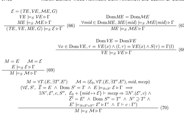
Before we can establish a static interpretation type soundness property, we first define a type consistency relation that relates interpretation environments, target language contexts, and substitutions providing concrete types for type variables that are considered abstract by elaboration. Due to the presence of higher-order parameterised modules, we shall make use of a logical relation argument [Tait 1967], which links the relation itself to the static interpretation. The relation is given by a number of inference rules, which are listed in Figure 13. The rules allow inferences among sentences of the forms (1) 𝐸 |=𝑆 ℰ ◁ Γ, (2)

ME |=𝑆ℳ𝐸 ◁ Γ, (3) 𝑀 |=𝑆ℳ ◁ Γ, and (4) VE |=𝑆 𝒱𝐸 ◁ Γ. An essential property of the rules

is that they are decreasing, structurally, in their left argument and therefore define a well-formed inductive relation. The two most interesting rules are Rule68, which relates variables in elaboration and static interpretation environments with labels in target environments, and Rule70, which relates parameterised modules in elaboration and static interpretation environments through static interpretation from appropriately related environments to resulting appropriately related results.

Based on the established consistency relation, we can now state a general property establishing (1) that static interpretation is possible and terminates for all elaborating programs and (2) that generated target programs are appropriately typed.

Module Expressions. ℰ ⊢ mexp ⇒ Ψ ℰ ⊢ mdec ⇒ ∃𝑁.(ℰ′_{, 𝑐)} ℰ ⊢ { mdec } ⇒ ∃𝑁.(ℰ′_{, 𝑐)} (54) ℰ(mid) = ℰ′ ℰ ⊢ mid ⇒ ∃∅.(ℰ′_{, 𝜖)} (55) ℰ′_{(mid) = ℰ}′′ ℰ ⊢ mexp ⇒ ∃𝑁.(ℰ′_{, 𝑐)} ℰ ⊢ mexp . mid ⇒ ∃𝑁.(ℰ′′_{, 𝑐)} (56) ℰ ⊢ mty ⇒ ∃𝑇.𝐸 𝑇 ∩ names(ℰ ) = ∅ ℰ + {mid ↦→ 𝐸} ⊢ mexp : Σ 𝐹 = ∀𝑇.(𝐸, Σ) Φ = (ℰ , 𝐹, 𝜆mid ⇒ mexp)

ℰ ⊢ 𝜆mid : mty → mexp ⇒ ∃∅.Φ (57)

ℰ ⊢ mexp ⇒ ∃𝑁.(ℰ′_{, 𝑐) (𝑁 ∪ 𝑁}′_{) ∩ names(ℰ ) = ∅ 𝑁 ∩ 𝑁}′_{= ∅} ℰ(longmid) = (ℰ0, 𝐹, 𝜆mid ⇒ mexp′) (𝐸′, ∃𝑇′.𝐸′′) ≤ 𝐹 𝑇′⊆ 𝑁′

⊢ ℰ′_{:: 𝐸}′_{⇒ ℰ}′′ _ℰ

0+ {mid ↦→ ℰ′′} ⊢ mexp′⇒ ∃𝑁′.(ℰ′′′, 𝑐′)

ℰ ⊢ longmid( mexp ) ⇒ ∃(𝑁 ∪ 𝑁′_).(ℰ′′′_{, 𝑐 ; 𝑐}′₎ (58)

Module Declarations. ℰ ⊢ mdec ⇒ ∃𝑁.(ℰ′_{, 𝑐)}

mdec = dec ℰ ⊢ dec ⇒ ∃𝑁.(ℰ′_{, 𝑐)} ℰ ⊢ mdec ⇒ ∃𝑁.(ℰ′_{, 𝑐)} (59) ℰ ⊢ ty : 𝜏

ℰ ⊢ type tid = ty ⇒ ∃∅.({tid ↦→ 𝜏 }, 𝜖) (60) ℰ ⊢ mexp ⇒ ∃𝑁.(Φ, 𝑐)

ℰ ⊢ module mid = mexp ⇒ ∃𝑁.({mid ↦→ Φ}, 𝑐) (61) ℰ ⊢ 𝜖 ⇒ ∃∅.({}, 𝜖) (62) ℰ ⊢ mty : Σ ℰ′_{= {mtid ↦→ Σ}}

ℰ ⊢ module type mtid = mty ⇒ ∃∅.(ℰ′_{, 𝜖)} (63)

ℰ ⊢ mexp ⇒ Ψ ℰ ⊢ open mexp ⇒ Ψ (64) 𝑁1∩ (names(ℰ) ∪ 𝑁2) = ∅ ℰ ⊢ mdec1⇒ ∃𝑁1.(ℰ1, 𝑐1) ℰ + ℰ1⊢ mdec2⇒ ∃𝑁2.(ℰ2, 𝑐2) ℰ ⊢ mdec1 mdec2⇒ ∃(𝑁1∪ 𝑁2).(ℰ1+ ℰ2, 𝑐1 ; 𝑐2) (65) Fig. 12. Static interpretation rules for module expressions and module declarations.

Proposition 6.1. (Static Interpretation Normalisation and Type Soundness) If 𝐸 ⊢ mdec : ∃𝑇.𝐸′ and 𝐸 |=𝑆 ℰ ◁ Γ then there exists 𝑁 , ℰ′, 𝑐, Γ′, and 𝑆′ such that ℰ ⊢ mdec ⇒

∃𝑁.(ℰ′_{, 𝑐) and 𝑁 ⊇ 𝑇 and Dom 𝑆}′_{= 𝑇 and 𝐸}′_|=

𝑆∘𝑆′ℰ′◁ Γ′ and Γ ⊢ 𝑐 : Γ′.

Proof. By mutual induction over mdec and mexp. □

The following corollary expresses a simplified version of the above proposition.

Corollary 6.2. (Top-level Normalisation and Type Soundness) If ⊢ mdec : {𝑥 : i32} then there exists 𝑁 , 𝑙, 𝑐, and Γ such that ⊢ mdec ⇒ ∃(𝑁 ∪ {𝑙}).({𝑥 ↦→ (𝑙, i32)}, 𝑐) and ⊢ 𝑐 : Γ + {𝑙 ↦→ i32}.

ℰ = (TE , 𝒱𝐸, ℳ𝐸, 𝐺) VE |=𝑆 𝒱𝐸 ◁ Γ ME |=𝑆 ℳ𝐸 ◁ Γ (TE , VE , ME , 𝐺) |=𝑆 ℰ ◁ Γ (66) DomME = Domℳ𝐸

∀mid ∈ DomME , ME (mid) |=𝑆 ℳ𝐸(mid) ◁ Γ

ME |=𝑆ℳ𝐸 ◁ Γ (67) DomVE = Dom𝒱𝐸 ∀𝑥 ∈ DomVE , 𝜏 = VE (𝑥) ∧ (𝑙, 𝜏 ) = 𝒱𝐸(𝑥) ∧ 𝑆(𝜏 ) = Γ(𝑙) VE |=𝑆 𝒱𝐸 ◁ Γ (68) 𝑀 = 𝐸 ℳ = ℰ 𝐸 |=𝑆 ℰ ◁ Γ 𝑀 |=𝑆 ℳ ◁ Γ (69) 𝑀 = ∀𝑇.(𝐸, ∃𝑇′.𝐸′) ℳ = (ℰ0, ∀𝑇.(𝐸, ∃𝑇′.𝐸′), mid, mexp) (∀ℰ , 𝑆′, ℰ = 𝐸 ∧ Dom 𝑆′= 𝑇 ∧ 𝐸 |=𝑆∘𝑆′ ℰ ◁ Γ =⇒ ∃𝑁′_{, ℰ}′_{, 𝑐, 𝑆}′′_{, ℰ} 0+ {mid ↦→ ℰ } ⊢ mexp ⇒ ∃𝑁′.(ℰ′, 𝑐) ∧ ℰ′_{= 𝐸}′ _{∧ Dom 𝑆}′′_{= 𝑇}′ _{∧ 𝑁}′_{⊇ 𝑇}′ _∧ 𝐸′ |=𝑆∘𝑆′_∘𝑆′′ℰ′◁ Γ′ ∧ Γ ⊢ 𝑐 : Γ′) 𝑀 |=𝑆 ℳ ◁ Γ (70)

Fig. 13. Type consistency logical relation.

With local module declarations, mdec may contain both higher-order module declarations and complex applications of such modules. This corollary thus illustrates a non-trivial property, similar to showing for the simply-typed lambda calculus that if ⊢ 𝑒 : i32 then there exists an integer 𝑑 such that 𝑒 ˓→*𝑑. Notice also that, because the target language contains no local bindings, all declared labels in 𝑐 escape to top-level and are described by the resulting context Γ + {𝑙 ↦→ i32}.

7 TYPE INFERENCE FOR THE MODULE LANGUAGE

We shall not here give a type inference algorithm for the module language but instead mention that type inference for the language becomes straightforward (i.e., syntax directed) if elaborated module types are what is called type explicit [Milner et al. 1997].

The notion of type explication is mutually inductively defined as follows. A module type Σ = ∃𝑇.𝐸 is type explicit if 𝐸 is type explicit and for all 𝑡 ∈ 𝑇 , there exists a longtid such that 𝐸(longtid) = 𝑡. A module type Σ = ∃𝑇.𝐹 is type explicit if 𝑇 = ∅ and 𝐹 is type explicit. A parameterised module type 𝐹 = ∀𝑇.(𝐸, Σ) is type explicit if ∃𝑇.𝐸 is type explicit. An environment 𝐸 is type explicit if all module types Σ in 𝐸 are type explicit.

The importance of type explication becomes apparent when trying to match a concrete environment 𝐸′ against a module type Σ = ∃𝑇.𝐸, which is what is required in the rule for application of parameterised modules. If Σ is type explicit, it becomes straightforward to decide whether there exists a substitution 𝑆 such that Dom 𝑆 = 𝑇 and 𝑆(𝐸′) ≻ 𝐸.

The following proposition states that our language for specifying module types generates type explicit module types:

Proposition 7.1. (Type Explicit Module Types). If 𝐸 ⊢ mty : Σ or 𝐸 ⊢ spec : Σ then Σ is type explicit if 𝐸 is type explicit.

There are a number of good reasons for extending the language for expressing module types [Ramsey et al. 2005] to avoid unnecessary duplication of module type specification code. As long as such extensions come with guarantees that every expressible module type is type explicit, type inference for the module language will be straightforward.

8 POLYMORPHISM AND HIGHER-ORDER FUNCTIONS

In this section, we show how certain classes of polymorphic functions and polymorphic types at the source level can be treated as derived forms of parameterised modules and how certain instantiations can be treated as parameterised module applications.

8.1 Polymorphic Functions

Consider the following Futhark declaration of a function polymorphic in the types t and s: let imap ’t ’s (f: (i32,t)→s) (a:[]t) : []s =

map f (zip (iota (length a)) a)

This declaration can be treated as a special derived form of a declaration of a parameterised module:

module Imap (X: {type t type s val f: (i32,t)→s}) = { open X

let imap (a:[]t) : []s = map f (zip (iota (length a)) a) }

Now, for obtaining an instantiation of the module, it is possible to instantiate the “polymor-phic function” imap to concrete arguments as follows:

let main () = imap (𝜆(i,x)→i+x) [1,2,3]

This code can then be translated into the following modularised code:

local module Imap_23 = Imap({type t=i32 type s=i32 let f (i,x) = i+x}) in { let main () = Imap_23.imap [1,2,3] }

This special short-hand for instantiating “polymorphic functions” is possible only in certain cases. For simplicity, it can be required that type parameter instantiations can be determined directly from the calling context and that the free variables of the passed arguments (e.g., the free variables in𝜆(i,x)→i+x) are all bound outside the containing module declaration. With a little more bookkeeping, it is possible to relax this requirement by implementing a version of lambda lifting [Johnsson 1985] that adds additional parameters to the declared function. Finally, with this approach, it is a requirement that the declared polymorphic functions do not themselves return functions; the scheme can support a number of higher-order functions but not first-class functions in general.

8.2 Polymorphic Types

Consider the following Futhark declaration of a “polymorphic type”: type pair ’t ’s = (t,[]s)

This type declaration can be translated into the following module declaration: module Pair (X : {type t type s}) =

open X

type pair = (t,[]s) }

For obtaining an instantiation of the module, it is possible to instantiate the “polymorphic type” pair to concrete arguments as follows:

type y = pair i32 bool

This code can be translated into the following module-level declaration: local module Pair_33 = Pair({type t=i32 type s=bool}) in { type y = Pair_33.pair }

Although this technique has some limitations compared to supporting polymorphism at the core language level, the mechanism is simple and can, for certain application domains, relieve the language implementor from considering polymorphism at the core language level. In practice, Futhark is relying on separate passes for eliminating core language polymor-phism and higher-order functions [Hovgaard 2018]. These passes both occur after static interpretation of modules and do not interfere with static interpretation. The separation of the passes for core language monomorphication and core language elimination of higher-order functions from static interpretation allows for supporting a richer set of polymorphic higher-order functions.

9 FORMALISING THE DEVELOPMENT IN COQ

We have formalised, in the Coq proof assistant, essential parts of the definitions given in this paper along with the proof of static interpretation normalisation. In the course of the development, we have used additional axioms of functional extensionality and proof irrelevance for propositions. Also, for the development of nominal techniques, we assume a countably infinite set of variable names.

We have taken an extrinsic approach [Benton et al. 2012], as opposed to an intrinsic one, to the representation of the core language, the module language, and the target language, which keeps our implementation close to the approach presented in the paper. The extrinsic encoding has an advantage of being more suitable for code extraction to obtain a certified implementation. That is, we have implemented the abstract syntax as simple inductive data types and given separate inductive definitions for relations such as elaboration, typing, and so on. The semantic objects of Figure4have been implemented as mutually defined inductive types using Coq’s with clause. The same approach is used for definitions of relations on environments. As described in Section4, semantic objects are represented using finite maps and sets and indeed, the implementation makes use of Coq’s standard library implementations of such objects. Specifically, we use the FMapList and FSetList implementations of the FMapand FSet interfaces, respectively. Both FMapList and FSetList make use of the listdata type together with a property that the list is ordered according to a strict order on the underlying data structure. The strict order for the underlying list allows us to prove an extensionality property for environments and sets (assuming proof irrelevance). That is, for any two environments 𝐸1 and 𝐸2 we have (∀𝑘, 𝐸1(𝑘) = 𝐸2(𝑘)) → 𝐸1 = 𝐸2. The equal sign = refers to the Coq propositional equality, which means that we can use all the standard rewriting machinery instead of using setoid equality.

Unfortunately, we cannot use the definition of environments from the standard library to define semantic objects such as MEnv because of Coq’s limitation that using type constructors for the environments from the standard library will violate Coq’s strict positivity check for inductive definitions. To overcome this complication, we introduce an isomorphic pair-of-vectors representation of environments, where the first vector is an ordered vector of keys and the second vector is a vector of values. Separating keys and values in different vectors allows