Three Essays on Polarization
Thèse ANDRÉ-MARIE TAPTUE Doctorat en économique Philosophiæ doctor (Ph.D.) Québec, Canada ©ANDRÉ-MARIE TAPTUE, 2015Résumé
Cette thèse porte sur la comparaison de la polarisation dans les distributions de revenu et est organisée en quatre chapitres. L’importance d’étudier la polarisation provient des risques de tensions sociales qui peuvent survenir dans une économie polarisée en plus de l’effritement de sa classe moyenne et les conséquences néfastes sur le développement économique. Le premier chapitre procède à une revue des différents travaux qui traitent de la polarisation. Certains de ces travaux établissent les fondements pour la mesure de la polarisation et la distinction avec la mesure des inégalités tandis que d’autres analysent les différentes manières de considérer les distances et les disparités entre individus et la façon dont la polarisation peut être mesurée dans une perspective économique, sociale et socio-économique. Ce premier chapitre distingue cinq types de polarisation : la polarisation du revenu, la bi-polarisation, la polarisation sociale, la polarisation socio-économique et la polarisation multidimensionnelle.
Le deuxième chapitre prend en compte les deux composantes de la polarisation que sont l’aliéna-tion et l’identifical’aliéna-tion pour développer une méthode de dominance stochastique en polarisal’aliéna-tion. Cette méthode est appliquée pour comparer la polarisation entre 16 pays et les USA pris comme pays de référence, en utilisant les données du Luxembourg Income Study (LIS). Certains pays comme le Danemark, la Norvège ou la Suisse affichent moins de polarisation que les USA tandis que les USA affichent moins de polarisation que l’Espagne, l’Italie et la Grèce.
Le troisième chapitre considère uniquement la composante aliénation dans les indices de po-larisation et développe une approche pour comparer la taille de la classe moyenne dans deux distributions de revenu. La comparaison des distributions de revenu est établie pour une classe d’indices de polarisation indépendants de la composante identification et dont le développement conduit à l’introduction de surfaces de dominance en aliénation. Une distribution possédant une grande surface de dominance en aliénation est plus concentrée dans les extrêmes et possède une classe moyenne de petite importance. Une application numérique permet de comparer l’effrite-ment de la classe moyenne des distributions de revenus de 22 pays à l’aide des données du LIS. Il en ressort que les USA ont une classe moyenne plus importante que le Mexique et le Pérou
mais moins importante que le reste des pays.
Le quatrième et dernier chapitre s’intéresse à la dimension identification dans les indices de polarisation et dérive une classe d’indices pouvant être utilisés pour mesurer le degré d’homo-généité dans une distribution de revenu. Le développement aboutit à des courbes de dominance qui peuvent être utilisées pour déterminer si l’homogénéité ou le degré de similarité est plus élevé dans une distribution que dans une autre. Cette méthodologie est utilisée pour comparer l’homogénéité des distributions de revenus de 11 pays en utilisant les données du LIS. Cette application montre que les USA sont plus homogènes que le Mexique et le Pérou mais moins homogènes que tous les autres pays.
Abstract
This thesis addresses the problem of polarization comparison and is organized in four chapters. A motivation to study polarization stems from the risk of social unrest that may arise in a polarized society along with the disappearance of its middle class and the negative consequences on the economic development. The first chapter reviews the basic conceptual foundations for the measurement of polarization, the origins of those foundations, how polarization is distinct from inequality and other ways of considering distances and differences across individuals, and how polarization can be measured in an economic, a social, and a hybrid socioeconomic perspective. It distinguishes five different types of polarization: income polarization, bi-polarization, social polarization, socio-economic polarization and multidimensional polarization.
The second chapter develops a method of stochastic dominance in polarization accounting sep-arately for the two basic components of polarization, namely alienation and identification. The methodology establishes a robust comparison of polarization based on the variations of alien-ation and identificalien-ation thresholds and is applied to data from seventeen countries taking the USA as a benchmark to which are compared the other 16 countries. Data are drawn from the Luxembourg Income Study database. As a result, stochastic dominance can hold in either di-rection since some countries like Denmark, Norway or Switzerland stochastically dominate the USA and the USA stochastically dominates other countries like Spain, Italy or Greece.
The third chapter shows how to compare the size of the middle class in income distributions using only the alienation component of polarization. We derive a class of polarization indices where the antagonism function is constant in identification. The comparison of distributions using an index from this class motivates the introduction of an alienation dominance surface, which is a function of an alienation threshold. We first prove that a distribution has a large alienation component in polarization compared to another if it always has a larger dominance surface regardless of the value of the alienation threshold. Then, we show that the distribution with a large dominance surface is more concentrated in the tails and has a smaller middle class than the other distribution. An empirical illustration with the distributions of twenty-two
countries from the Luxembourg Income Study database shows that the USA has a higher middle class than Mexico and Peru and a smaller middle class than the rest of the countries.
The fourth and last chapter develops a methodology to compare the degree of homogeneity of two income distributions using only the identification component of polarization. This develop-ment leads to identification dominance curves and derives first-order and higher-order stochastic dominance conditions. Dominance curves are used to determine whether identification, homo-geneity, or similarity of individuals is greater in one distribution than in another for general classes of polarization indices and ranges of possible identification thresholds. Our methodology is illustrated by comparing pairs of distributions of eleven countries drawn from the Luxem-bourg Income Study database. This application shows that the USA is more homogeneous than Mexico and Peru and less homogeneous than the other countries.
Contents
Résumé iii Abstract v Contents vii List of Tables ix List of Figures xi Remerciements xvii Introduction 1 1 Polarization 5 1.1 Introduction . . . 5 1.2 Motivation . . . 8 1.3 Notation . . . 12 1.4 Income Polarization . . . 13 1.5 Bi-polarization . . . 22 1.6 Social polarization . . . 44 1.7 Socio-economic polarization . . . 49 1.8 Multidimensional Polarization . . . 57 1.9 Polarization in Practice . . . 60 1.10 Conclusion . . . 642 Stochastic dominance in polarization 67 2.1 Introduction . . . 67
2.2 Literature . . . 69
2.3 Principle of stochastic dominance in polarization . . . 72
2.4 Application . . . 81
2.5 Conclusion and extensions . . . 88
3.1 Introduction . . . 93
3.2 Methodology . . . 95
3.3 Case of income distributions . . . 102
3.4 Application . . . 109
3.5 Estimation and inference . . . 114
3.6 Conclusion . . . 130
4 Comparing the homogeneity of income distributions using polarization indices 133 4.1 Introduction . . . 133
4.2 Identification in polarization measures . . . 135
4.3 Stochastic dominance . . . 136
4.4 Case of income distributions . . . 142
4.5 Estimation and inference . . . 143
4.6 Empirical illustration using LIS data . . . 149
4.7 Conclusion . . . 156 Conclusion 157 A Appendix chapter 2 159 B Appendix chapter 3 165 C Appendix chapter 4 169 Bibliography 175
List of Tables
1.1 A categorization of polarization indices . . . 66
2.1 Sample sizes, mean and median incomes. Year=2004. . . 84
3.1 Sample sizes, mean and median income for 22 countries. Year=2004. . . 110
3.2 Result of the alienation dominance between 22 countries . . . 114
3.3 Critical frontiers and corresponding p-values of the tests between the USA and other countries at the significance level of 5% . . . 130
4.1 Sample sizes, mean and median income for 11 countries. Year=2004. . . 150
4.2 Result of identification dominance between 11 countries based on their identifica-tion dominance curves . . . 153
List of Figures
1.1 Merging two relatively small and close groups at the average of their incomes
increases polarization. . . 15
1.2 Moving 𝑥 towards 𝑦 increases polarization. . . 16
1.3 Absorption of the middle class into richer and poorer classes increases polarization. 17 1.4 A squeeze of a basic density does not increase polarization . . . 18
1.5 A double squeeze cannot reduce polarization . . . 19
1.6 A symmetric outward slide must raise polarization . . . 20
1.7 Finding the size 𝑀 of the middle class with a density function . . . 24
1.8 Finding the size 𝑀 of the middle class with a cumulative distribution function . 24 1.9 Lorenz curve and the Levy(1987) index of the size of the middle class . . . 25
1.10 Quantile function . . . 26
1.11 Increased spread . . . 27
1.12 Increased bi-polarity . . . 28
1.13 First-order bi-polarization curves . . . 30
1.14 Second-order bi-polarization curve . . . 31
1.15 Average distance from bipolar extremes . . . 33
1.16 Maximum bi-polarization . . . 36
1.17 Polarization, relative median deviation and withgroup and between-group in-equality . . . 38
1.18 Does increasing bi-polarity increase polarization? . . . 39
1.19 Fractionalization (𝐹 𝑅𝐴𝐶) and social polarization (𝑅𝑄) indices as a function of a number of equally-sized groups . . . 49
1.20 A slide of basic densities within a group increases socio-economic polarization . . 52
1.21 A smaller group becoming less radical and a bigger group becoming more radical does not decrease socio-economic polarization . . . 53
1.22 A hypothetical distribution of health statuses across two different social groups (Males and Females) — the initials stand for: Very Poor (VP), Poor (P), Fair (F), Good (G) and Very Good (VG) . . . 55
1.23 A hypothetical distribution of health statuses across two different social groups (Males and Females) — the initials stand for: Very Poor (VP), Poor (P), Fair (F), Good (G) and Very Good (VG) . . . 55
1.24 Polarization (measured by the 𝐷𝐸𝑅(𝛼 = 1) index) and inequality for 21 countries, LIS Wave 3 . . . 62
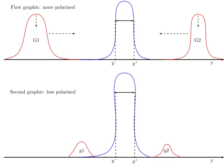
2.1 An illustration of the problem of depolarization in two periods: Individuals in groups 𝐺1 and 𝐺2 are displaced into the interval [𝑦−, 𝑦+] and the result is the
second graphic with groups 𝑔1 and 𝑔2 smaller than G1 and G2 and close to [𝑦−, 𝑦+]. 74
2.2 Dominance surface in polarization at 𝑧𝑎 and 𝑧𝜄 for a population 𝐴 (𝐻𝐴(𝑧𝑎, 𝑧𝜄)): Proportion of individuals in 𝐴 for whom alienation is greater than 𝑧𝑎 and
identi-fication greater than 𝑧𝜄. . . 75
2.3 Increasing distances increases antagonism: The distance of a group from the
me-dian has increased, but its density has not changed . . . 77
2.4 Increasing identification increases antagonism. The density of a group has
in-creased, but its distance from the median has not changed . . . 78
2.5 Increasing identification with greater distances increases antagonism: The density
of a group has increased together with the increase of its distance from the median. 78
2.6 Mean and median income (in thousands of $US) of 17 countries . . . 85
2.7 Difference between dominance surfaces of the USA and Spain, and the USA and
Ireland . . . 86
2.8 Difference between dominance surfaces of the USA and Mexico, and the USA and
Canada . . . 87
2.9 Difference between dominance surfaces of the USA and other countries . . . 89
3.1 Alienation dominance surface for a population 𝐴 . . . 103
3.2 Increased spread increases bi-polarization and alienation dominance surface
re-gardless of alienation threshold . . . 105
3.3 Increased bi-polarity can increase (case 1) or decrease (case 2) the alienation
dominance surface . . . 106
3.4 Increased bi-polarity can have an ambiguous effect on the alienation dominance
surface . . . 106
3.5 Curves of the alienation dominance surface and the size of the middle class as a
function of alienation thresholds . . . 108
3.6 Finding the value 𝑧∗
𝑎 of the alienation threshold for which 𝐻(𝑧∗𝑎) = 𝑀 (𝑧𝑎∗) . . . . 108
3.7 Mean and median income (thousands of $ US) of 22 countries . . . 111
3.8 Curves of the difference between the alienation dominance surface of the USA and
those of other countries multiplied by 100 . . . 113
3.9 Alienation dominance curves between Peru, Poland and Austria, and between
USA, Spain and Slovenia . . . 115
3.10 Critical frontiers and the interval of dominance of distribution 𝐴 by distribution 𝐵 117
3.11 Density curves showing the convergence of 𝐻(𝑧̂ 𝑎) when 𝑧𝑎= 0.5. For each size 𝑁 , 1,000 samples are drawn from a log-normal distribution of mean zero and
standard deviation 1 . . . 118
3.12 Density curves of𝐻(𝑧̂ 𝑎) when 𝑧𝑎= 0.2, 0.5, 1, and 1.5. For sizes 𝑁 = 1, 000; 5, 000 and 10, 000; 1,000 samples are drawn from a log-normal distribution of mean zero and standard
deviation 1 . . . 118
3.13 Graphical illustration of a statistical test with p-values at different alienation
3.14 Alienation dominance curves and p-values at different alienation thresholds for
the USA and Mexico, and the USA and Peru . . . 122
3.15 Alienation dominance curves and p-values at different alienation thresholds for
the USA and: Greece, Ireland, Italy and Spain . . . 124
3.16 Alienation dominance curves and p-values at different alienation thresholds for the USA and: Austria, Canada, Czech Rep, Luxembourg, Poland, Switzerland,
Slovenia and Slovak Rep . . . 126
3.17 Alienation dominance curves and p-values at different alienation thresholds for
the USA and: Denmark, Findland, Germany, Netherlands and Norway . . . 127
3.18 Alienation dominance curves and p-values between the USA and Estonia, and the
USA and UK at different alienation thresholds . . . 128
4.1 Reducing group sizes also reduces identification: A society composed of few groups of large sizes has more identification than a society composed of many groups of
small sizes. . . 135
4.2 Identification dominance curves for two distributions 𝐴 and 𝐵 . . . 141
4.3 Identification dominance curve for 𝑧𝜄, 𝐻(𝑧𝜄): Proportion of individuals whose
income density (identification) is greater than 𝑧𝜄 . . . 143
4.4 Density curves showing the convergence of 𝐻(𝑧̂ 𝜄) when 𝑧𝜄 = 0.00002. For each sample size 𝑁 , 1000 samples are drawn from a log-normal distribution of mean
zero and standard deviation 1 . . . 145
4.5 Graphical illustration of a statistical test with p-value at different identification
thresholds . . . 149
4.6 Identification dominance curves and p-values for Mexico, Peru and the USA . . . 154
4.7 Identification dominance curves and p-values for Canada, Denmark, Finland,
A la mémoire de mon grand frère Kwiate Fidèle Emmanuel
Remerciements
Si la décision de s’engager dans des études doctorales est généralement personnelle et dépend de l’étudiant, la conduite de la thèse à son terme nécessite un encadrement qui est indispensable. Ainsi, l’accomplissement de ce projet que j’ai engagé en 2009 n’aurait jamais été possible sans l’encadrement du professeur Jean-Yves Duclos à qui j’adresse ici tous mes remerciements et ma sincère gratitude.
Je voudrais également adresser mes remerciements à tous les professeurs du département d’économique de l’Université Laval et en particulier aux professeurs Charles Bellemare et Sylvain Eloi Dessy pour leur disponibilité à me prodiguer des conseils, des encouragements et des orientations pour mes travaux.
Merci à tous les participants au congrès de ECINEQ à Bari en Italie en 2013, en particulier au professeur Gordon Anderson pour ces commentaires qui m’on aidé à améliorer mes travaux. Pour le soutien technique dans les logiciels statistiques, je voudrais remercier Abdelkrim Araar et ma camarade Maria Lopera.
A tous mes camarades au programme de doctorat en économique à l’Université Laval, merci de l’ambiance créée, de la collaboration et du soutien mutuel que nous nous sommes toujours donné dans nos travaux respectifs.
A mes parents, tous mes frères, mes soeurs, tous les membres de ma famille et en particulier mes grands frères Ndefo Louis et Taptué Félix, et à mes mamans Tokam Marguérite et Kwiate Marie Thérèse, je dis merci pour tout le soutien et les encouragements.
A mon ami et frère Tchana Tchana Fulbert, son fils Steve et son épouse Judith, merci de l’accueil que vous m’avez réservé à mon arrivée à Québec, de l’encadrement et des conseils que vous m’avez donnés pour mon intégration et la poursuite des mes études.
soutiens respectifs et les échanges fructueux que nous avons eus pendant cette période.
Pour mener à bien ces études de doctorat, j’ai bénéficié des bourses du département d’économique, du CIRPEE, du BBAF, du Fonds Georges-Henri-Lévesque et des fonds de recherche FQRSC et CRSH de mon professeur Jean-Yves Duclos. A tous ces organismes de financement, j’adresse mes sincères remerciements.
Pour terminer, j’aimerais souligner le soutien inconditionnel de trois personnes qui ont joué un rôle essentiel pendant les années que j’ai passées à faire cette thèse: il s’agit de mon épouse Jeannette, ma fille Gracia Aurelle et mon fils Christ Michael qui m’ont toujours encouragé et soutenu dans des moments difficiles. Je leur suis extrêmement reconnaissant et de tout coeur, je leur dis merci.
Introduction générale
Les distributions de revenus sont généralement comparées dans le domaine des inégalités en utilisant l’indice de Gini et les courbes de concentration. Des auteurs récents tels que Thomas Piketty (Piketty,2013) centrent leurs analyses sur le revenu des 1% les plus riches. En focalisant sur l’aspect des inégalités, ces mesures ne captent pas certaines conséquences indésirables telles l’effritement de la classe moyenne et les conflits sociaux qui peuvent survenir dans une mauvaise distribution du revenu. Esteban and Ray(1994) affirment que l’étude des inégalités ne distingue pas entre la convergence vers la moyenne globale et la convergence vers les moyennes locales dans une distribution de revenu. Le phénomène de polarisation, qui apparaît lorsque la distri-bution de revenu conduit à la formation de deux ou plusieurs groupes antagonistes, distingue ces deux formes de convergence et peut être plus approprié par exemple lorsqu’on étudie les différences entre les pays en terme de revenu. Par exemple, la convergence des économies du Nord vers un taux de croissance distinct de celui vers lequel convergeraient ceux du Sud décrit un comportement de l’économie mondiale que l’étude des inégalités pourrait ne pas permettre d’appréhender, mais que les études de la polarisation permettrait de mieux cerner. Foster and
Wolfson(2010/1992) etWolfson(1994) soutiennent que certaines formes de transferts progressifs
au sens de Pigou-Dalton réduisent les inégalités mais augmentent la polarisation. Lorsque les transferts conduisent à une convergence des revenus de part et d’autre de la médiane vers leurs moyennes respectives, les inégalités diminuent et la bi-polarisation augmente.
Par ailleurs, Esteban and Ray (1994, 1999) établissent un lien de cause à effet entre la polar-isation et les tensions sociales. La polarpolar-isation est vue comme une des causes des conflits qui surviennent lorsque des groupes d’intérêt se disputent un bien public et que les membres de chaque groupe contribuent financièrement à l’effort de leur groupe pour s’accaparer une grande partie du bien public. Dans cette situation, les transactions économiques, le commerce, les pouvoirs politique et économique peuvent être restreints aux membres d’un même groupe, les dépenses publiques pourraient favoriser certains groupes de personnes et le développement des infrastructures publiques pouurait être biaisé.
D’autre part, les pauvres deviennent plus pauvres et les riches plus riches dans une économie polarisée; il y a effritement de la classe moyenne avec des conséquences négatives sur le développe-ment économique dans la mesure où la classe moyenne est perçue comme la principale source de la main d’œuvre et de la population active (Foster and Wolfson, 2010/1992), comme celle qui contribue largement aux revenus d’impôt d’un pays et celle dont la possession d’une grande part du revenu national est associée à une croissance économique forte (Easterly,2001).
Les mesures publiques qui affectent les distributions de revenu et entrainent la formation des groupes antagonistes devraient, au vu de ces conséquences, évaluer et comparer la polarisa-tion dans les nouvelles distribupolarisa-tions à celle qui existe déjà. Cette comparaison permettrait d’implémenter les mesures qui génèrent moins de polarisation du revenu et réduisent le risque de tensions sociales.
Les trois essais de cette thèse sont organisés dans quatre chapitres et centrés sur les méthodes de comparaison de la polarisation et de ses différentes composantes, à l’exception du premier essai qui fait une revue des différents travaux en polarisation.
Le Chapitre 1 qui forme le premier essai montre que le revenu n’est pas la seule dimension sous laquelle une société peut se polariser, faire face à l’effritement de sa classe moyenne et générer des conflits sociaux. Il existe la polarisation sociale où les groupes antagonistes sont formés sur la base des caractéristiques sociales comme la religion, l’ethnie, la couleur de la peau ou le niveau d’instruction. De même, à l’intérieur d’un groupe économique, les modérés peuvent se distinguer des radicaux, ce qui ouvre la voie à la polarisation multidimensionnelle mixant les dimensions du revenu et des caractéristiques sociales. Ce premier essai met également en exergue les éléments qui distinguent la polarisation et les inégalités. Par exemple, lorsque les transferts progressifs de revenus sont effectués de sorte que les individus en dessous et ceux au dessus de la médiane se concentrent chacun autour de la moyenne de leurs revenus, les inégalités diminuent et la polarisation augmente. De même, une distribution de revenu qui conduit à des groupes de très petites tailles ou encore celle dans laquelle tous les individus ont des revenus distincts, affiche une certaine inégalité mais n’est pas polarisée.
Le chapitre 2 forme le deuxième essai et développe une méthode de dominance stochastique en polarisation. Il s’agit d’une méthode robuste de comparaison des distributions amplement développée en pauvreté et inégalité, mais qui ne l’était pas encore en polarisation. Lorsque les indices utilisés dans la comparaison contiennent des paramètres arbitraires, la dominance stochastique permet d’établir un ordre partiel entre deux distributions indépendamment de ces paramètres.
Les chapitres 3 et 4 forment le troisième essai et traitent chacun d’une des composantes de la polarisation. Le chapitre 3 traite de l’hétérogénéité des distributions en utilisant un indice de polarisation dans lequel sont considérées uniquement les distances entre les revenus des différents groupes. La forme réduite de l’indice de polarisation obtenue dans ce cas mesure la taille de la classe moyenne et la concentration du revenu dans les queues de distribution. Le développe-ment théorique dans ce chapitre conduit à une surface de dominance en aliénation qui permet de comparer la classe moyenne dans deux distributions de revenu pour toute distance maximale possible fixée entre les revenus et la médiane. Le chapitre 4 étudie la composante homogénéité de l’indice de polarisation en négligeant les écarts entre les revenus des différents groupes. Le développement théorique dans cet ultime chapitre conduit à des courbes de dominance en iden-tification permettant de comparer l’homogénéité des distributions du revenu pour toute valeur maximale possible de la densité des groupes d’individus dans une économie polarisée. Ces deux chapitres du troisième essai font chacun abstraction de l’interaction entre les deux composantes de la polarisation et mesurent leurs effets de manière séparée sur la distribution du revenu. Les chapitres 2, 3 et 4 font l’objet d’une application numérique avec les données du Luxembourg Income Study: La dominance stochastique élaborée dans le chapitre 2 permet de comparer la polarisation dans 17 pays; les surfaces de dominance en aliénation au chapitre 3 permettent de comparer la taille de la classe moyenne dans 22 pays et les courbes de dominance en identification au chapitre 4 permettent de comparer l’homogénéité des distributions de revenu dans 11 pays. Les principaux résultats montrent qu’en dehors du Mexique et du Perou, tous les autres pays sont moins polarisés et affichent de grandes classes moyennes par rapport aux USA. Aussi, en dehors du Mexique et du Perou, tous les autres pays sont plus homogènes que les USA. En outre, les pays comme la Norvège, le Danemark ou la Suisse sont les plus homogènes et les moins polarisés.
Chapter 1
Polarization
1.1 Introduction
This chapter reviews the basic conceptual foundations for the measurement of polarization, the origins of those foundations, how polarization is distinct from inequality and other ways of considering distances and differences across individuals, and how polarization can be measured in an economic, a social and in a hybrid socio-economic perspective. The chapter focuses largely on concepts and measurement, with only cursory overviews both of the empirical polarization literature and of the theoretical polarization/conflict literature.
It is useful to stress at the outset that the term “polarization” means different things to different people. First, there are those people that view polarization as important for ethical reasons and those that consider polarization as instrumental towards generating tensions and conflicts. Second, there are different ‘types’ of polarization. The chapter distinguishes five such types: income polarization, income bi-polarization, social polarization, socio-economic polarization and multidimensional polarization. They are listed inTable 1.1along with their main distinguishing features — how they form groups and how they measure distances. Some of the relevant indices are also listed.
Income polarization
The chapter first discusses income polarization, understood as polarization over the univariate distribution of a cardinal variable of interest. This regards polarization as a clustering of that variable around an arbitrary number of local means. Variables of interest in that context usually measure welfare; income polarization is then polarization over the distribution of a measure of welfare. This measure of welfare is often income, which explains why the term ‘income
polarization’ is chosen to denote this class of polarization measures. The variable of interest can also be unrelated to welfare. One can think, for instance, of income polarization over a distribution of political attitudes or over a distribution of geographical locations. As long as these variables have cardinal value, polarization over them will be referred to as income polarization.
The formalization of income polarization has mostly relied in the literature on an identifica-tion/alienation framework. Members of the same group identify with each other; members of different groups feel alienation with respect to one another. Income polarization is assumed to be increasing in both aspects: the greater the level of group identification or the greater the level of alienation, the greater the level of polarization.
Bi-polarization
An alternative notion of polarization across a cardinal variable of interest is bi-polarization. Bi-polarization captures distances across two groups. These two groups have usually been defined as lying on either side of a median, thus taken as the middle of a distribution; for this reason, the bi-polarization literature is closely linked to the literature on the size of the middle class. But one can also think of bi-polarization as being concerned with the distance between two other separate income groups, such as the poor and the non-poor or the bourgeois and the proletarians. (Those two groups cannot, however, be defined by a variable other than the variable interest; using a variable other than the variable of interest to define groups would generate a measure of socio-economic polarization — see below.)
Two notions are intrinsic to the nature of bi-polarization: the notion of changes in spreads from the middle and the notion of variations in “bi-polarity”. An increase in the spreads of incomes from a middle position increases bi-polarization. An increase in bi-polarity — smaller income distances either among those below or among those above the middle — raises bi-polarization. Equivalently, a reduction in the income gaps between any two incomes, both above or below the median, increases bi-polarization.
The discussion until now already makes clear that the measurement of polarization generally involves both inequality-like and equality-like constituents. The equality-like constituent is the basis of the fundamental conceptual difference between inequality and polarization. Polarization differs from inequality in that the importance of pole (or group) homogeneity carries weight in addition to the importance of heterogeneity across individuals. Increased distances across individuals of different groups increase both inequality and polarization; increased bunching (for income polarization) or increased equality (for bi-polarization) across individuals of the same
group decreases inequality but raises polarization.
Much of the debate on the differences between inequality and polarization — and on the possible relevance of each in explaining conflict — effectively rests on the nature of the effects of Pigou-Dalton transfers on each of these measures of the income distribution. A regressive Pigou-Pigou-Dalton transfer increases bi-polarization if the transfer takes place across the median; however, such a transfer increases inequality but decreases bi-polarization if it occurs entirely on one side of the median.1 Whether either (or both) of these transfers increases conflict is a matter of debate; the polarization literature generally supports the view that a regressive same-side-of-the-median transfer actually reduces conflict.2
Social polarization
The chapter then turns to social polarization. Social polarization is concerned with polarization over variables that are qualitative or have no particular cardinal content. Social polarization does not use information on distances between individuals or groups: it only takes into account the size of the groups and sets distances between them to a constant. This is not to say that social polarization cannot measure tensions or distances across groups; it does this by focussing on the distribution of group sizes.
What matters for social polarization is not only how many groups there are, but also how salient their sizes are. The social polarization literature argues that, ceteris paribus, the larger the size of another group, the greater the threat felt by a given group (proportionally to the size of the other group). This introduces a fundamental distinction between inequality of 0/1 group membership (also called group fractionalization) and social polarization. Fractionalization increases when two identical groups split into two since there is then greater group membership inequality; social polarization falls following such a change.
Socio-economic and multidimensional polarization
Social polarization bases group identity on social characteristics; it sets distances to a binary 0/1 variable and thus does not make use of cardinal distance information. But a richer anal-ysis of differences across members of different social groups can also sometimes be performed jointly on social and economic indicators. Some income groups may be split along some social 1Note that there is also evidence in the welfare economics literature that, when asked about inequality, a
majority of respondents in various surveys believe that such same-side-of-the-median regressive transfers should also reduce inequality seeAmiel and Cowell(1992).
2For an exception to this, seeEsteban and Ray(2011a), where an increase in within-group inequality increases
conflict: increased inequality raises the likelihood that demonstrators within a group may be compensated for the cost of mobilization by other demonstrators within the same group.
characteristics; social groups can exhibit heterogeneity in welfare. The introduction of these joint dimensions leads to two generalizations, socio-economic polarization and multidimensional polarization.
Socio-economic polarization makes an asymmetric use of these dimensions. One set of social variables is used for group identification; a second set of economic variables fixes distances.3 Be-cause of this, the usual properties of the income polarization and income bi-polarization settings do not apply. In particular, bi-polarization properties of increasing spread and of increasing bi-polarity do not hold in a socio-economic polarization context.
Multidimensional polarization measures can also be designed. Group membership can be based on the entire set of social and economic characteristics; so can the measurement of distances across individuals. When this is done, a multidimensional analogue of unidimensional income polarization is obtained. Multidimensional polarization can also be of a socioeconomic type; this is achieved by defining social membership by social characteristics (as is usual) and by measuring distances on the basis of a multivariate distribution of welfare indicators.
1.2 Motivation
As for inequality, part of the motivation for studying polarization is ethical. Unlike inequality, however, the ethical motivation comes from the view that distances and differences across groups — as opposed to across individuals for inequality — are normatively undesirable. The hollowing out of the earnings distribution and the disappearance of the middle class may, for instance, create a more segregated and an intrinsically less good society.
Much of the motivation for the study of polarization also owes to the view that it is closely linked to the “generation of tensions, to the possibilities of articulated rebellion and revolt, and to the existence of social unrest in general” (Esteban and Ray 1994, p. 820). Linking group formation and the eruption of social unrest has a long history. Aristotle wrote (2350 years ago) that “it is manifest that the best political community is formed by citizens of the middle class, and that those states are likely to be well-administered, in which the middle class is large .. where the middle class is large, there are least likely to be factions and dissension” (Aristotle -350). To take just another prominent historical example, the Marxist critique of Hegel’s Philosophy (see for instance O’Malley and Blunden 1970) has forcefully argued that the emergence of two distinct social classes, the bourgeoisie and the proletariat, leads progressively to class struggles as societies industrialize. More generally, humanity’s history is often described as a series of
group struggles, those groups being typically fairly well defined according to socio-economic characteristics, interests and statuses.
The modern formal conceptualization of economic polarization along such antagonistic lines owes much toEsteban and Ray(1994) [ER]. Polarization is defined as the grouping of the population into significantly-sized clusters such that each cluster has members with similar attributes and different clusters have members with dissimilar ones. Views differ, however, on how to measure the importance and the relevance of such grouping and on how and whether, in particular, it is social or economic differences that matter in defining polarization. They also differ as to which of these differences is more likely to generate conflict.4
Consider first the case of social polarization. Ethnicity (broadly interpreted to include religious, racial and linguistic identities) is commonly perceived as an important source of it; ethnic groups are seen as firmly bounded, inclined toward ethnocentrism, hostile to outsiders and as exhibiting a belief that one’s ethnic group is centrally important. This can position ethnicity at the centre of politics and development in many societies — it is indeed frequent to observe political parties split along ethnic lines (Horowitz 1985). A social norm of equality further makes the subjugation of ethnic minorities illegitimate and spurs ethnic groups to compare their standing in society against that of other groups. With various technological and social developments, associated political divisions and resultant conflicts may also be increasingly common (Glaeser and Ward
2006).
The economic consequences of ethnic identities and of (potential or actual) conflict can be numerous (Montalvo and Reynal-Querol 2005a). Trust and trade may be restricted to individuals of the same ethnic group; public infrastructure may be ethnically biased; government transfers may disproportionately favor some ethnic groups, etc.
Underlying the above social tensions also clearly lies a diversity of economic statuses and inter-ests. It is in fact often argued that socio-political markers of tension are just proxies for more fundamental economic determinants of polarization (Creamer 2007). The evidence in McCarty
et al.(2006) suggest for instance that the increase in the divergence of economic interests of the
major constituencies of the two major American political parties may have led to an increase of polarization in American politics.
Theoretical demonstrations of the role of polarization in politics and governance can take a variety of forms. Rent seeking on the part of the different groups is one of them. Montalvo
and Reynal-Querol (2005b) presents a simple pure contest game in which agents seek rent by
4See for instance the 2008 special issue of the Journal of Peace Research on the linkages between polarization
spending resources in favor of a preferred group outcome. The utility distances across the groups are set to a constant and group sizes are assumed to be equal. The level of resources spent by agents affects the probability of success in the contest; that probability is equal to the share of each group in the total resources allocated to the contest. Because of the interaction between group sizes and group probabilities of contest success, the total resources allocated to the contest are shown to be a function of the social polarization index shown in Equation (1.33).
Polarization can also be modelled to lead to conflict in contexts in which distances across groups matter. A brief formalization of this takes the following form. Individuals in a given group derive greater utility from outcomes preferred by groups that are “closer” to them. The probability of a group implementing its preferred (ideal) outcome at the expense of other groups depends on the resources spent by the group in taking control. The sum of these resources also determines the importance of group conflict.
Outcomes of such a game have been studied in Esteban and Ray (1999). Increases in the utility distance between any pairs of groups lead to increases in social conflict. Conflict is always maximized on the symmetric bimodal distribution of the population. But there are many nonlinearities. For instance, a merger of two groups in a society with at least three social groups can increase or decrease conflict depending on the size of the merged groups as well as on the distribution of the population across the non-merged groups. A movement away from a symmetric distribution of three equally-sized groups to a symmetric two-group distribution initially decreases conflicts before it eventually increases it. Bunching — and not only spreads from a “middle” — emerges as an important determinant of conflicts.
A richer framework for studying both the occurrence and the intensity of conflicts and the effect of polarization and fractionalization in each case is found in Esteban and Ray (2008). In a highly polarized society, conflict is expensive, so that its appearance is rare. But when conflict occurs, it is intense. Less polarized societies, where conflict is less costly, witness a higher frequency of social unrest but of a more moderate intensity. Frequency and intensity can therefore be negatively correlated; it may be that the overall importance of conflict (frequency times intensity) may be reached at intermediate levels of polarization. The occurrence and the intensity of conflicts also depend crucially on the nature of the political system. For all these reasons, the precise overall relationship between polarization and conflict ends up being complex and nonlinear, even in relatively well structured theoretical settings.
Group distances and group identity affect differently inequality, social polarization and income polarization. Group cohesion and group distances can also influence differently the size of group conflict in an environment in which control over resources is partly determined by group action.
The most elaborate modeling of the linkages between conflict and features of group distance and identity is found in Esteban and Ray (2011b).
The game consists of fighting over a budget, a fraction of which is used for a public good and the rest of which is used for a private good. Each group has a most-preferred composition of public goods. An exogenous fraction of the budget is used for the public good; the precise allocation of that public good is endogenously determined by the identity of the winning group. A degree of group cohesion captures whether group payoffs, and not individual ones, are maximized. Group cohesion can be interpreted, for instance, as a degree of altruism or as an indicator of group leadership. Both of these features reinforce group cohesion and also provide possible answers to the important question of why individuals would want — or would need — to act in groups. Group members choose to make contributions to the resources used by their group to increase the group’s probability to win the game, seize control over the government’s budget and choose the allocation of the public good. In equilibrium, members of any given group make the same contribution; in equilibrium, the groups might be contributing different per capita levels of effort, but it is shown that this is not expected to affect significantly the value of aggregate conflict intensity. An approximately linear relationship is then established in Esteban and Ray (2011b) between equilibrium conflict intensity, the Gini index, fractionalization and polarization over differences in public good utilities. Four interesting polar cases emerge.
First, when all goods are private, utility distances across different group choices of public good allocations do not matter. This is because utility distances matter only when the allocation of public goods is important to groups. Only group sizes (and not group distances) drive conflict over the allocation of private goods. Distance-based indicators of divergences such as inequality and polarization do not predict conflict; it is only those indicators that are based solely on group size divergences (namely, fractionalization) that matter.
Second, when all goods are public, distances over preferences become salient, and the distance-influenced measures of polarization and inequality dominate fractionalization (which is invariant to group distances) as determinants of conflict. The degree to which polarization dominates inequality as a determinant of conflict depends on the strength of group cohesion; the greater the degree of group cohesion, the greater the conflict-determining importance of polarization as a measure influenced both by group sizes and by group distances.
Third, the relative importance of polarization and fractionalization depends on the importance of public goods. If public goods dominate the allocation of government spending, then conflict rests entirely on the value of winning the public goods allocation game. The importance of
polarization (which takes into account the utility distances across groups) then dominates the importance of fractionalization as a determinant of conflict since it alone takes into account public good utility distances across groups and therefore the value of competing for the precise allocation of that good.
Lastly, inequality has a negligible role when group cohesion is important and, more importantly, when population size is large (a large population makes individual action less effective). More generally, conflict arises only if population size is small (in which case inequality across indi-viduals is important because there are few interacting indiindi-viduals and individual action is thus important) or if there is group cohesion (in which case it is polarization and fractionalization — instead of inequality — that play an important role).
1.3 Notation
Before proceeding, it is useful to introduce the common notation that will be used in the different sections of the chapter. We denote income — or any other cardinal measure of welfare or, more generally, any cardinal measure of “locations” along which individuals can be found and that can therefore be used to measure distances across individuals — by 𝑦. Let 𝐹 (𝑦) be the cumulative distribution function (cdf) of income. 𝑝 = 𝐹 (𝑦) is the proportion of individuals in the population that enjoy a level of income that is less than or equal to 𝑦. We will often suppose the existence of a density function, which is the first-order derivative of a continuous cdf, denoted as 𝑓(𝑦)𝑑𝑦 = 𝑑𝐹 (𝑦). For discrete distributions, we will think of 𝑓(𝑦) as the relative frequency of an income of a value 𝑦.
We will denote quantiles as 𝑄(𝑝). For a strictly increasing continuous 𝐹 (𝑦), they can be defined as 𝐹 (𝑄(𝑝)) = 𝑝, or using the inverse distribution function, as 𝑄(𝑝) = 𝐹(−1)(𝑝). For discrete
distributions, 𝑄(𝑝) = 𝑖𝑛𝑓{𝑦 ∶ 𝑝 ≤ 𝐹 (𝑦)}. Thus, with a discrete distribution of 𝑁 incomes 𝑦𝑖, ranked in increasing values of 𝑦𝑖 such that 𝑦1≤ 𝑦2≤ 𝑦3≤ ... ≤ 𝑦𝑁−1 ≤ 𝑦𝑁, the quantiles are given by 𝑄(𝑝) = 𝑦𝑖, for (𝑖 − 1)/𝑁 < 𝑝 ≤ 𝑖/𝑁 and for 𝑖 = 1, ..., 𝑁 .
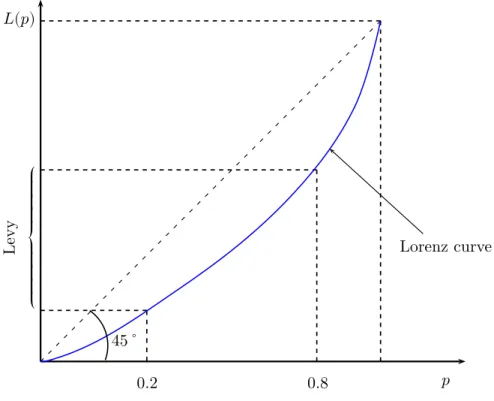
The median 𝑄(0.5) is denoted by 𝑚 and mean income by 𝜇. The mean-to-median ratio is given by 𝜇 = 𝜇/𝑚 and is a measure of the skewness of the distribution. Let̃ 𝑄(𝑞) = 𝑄(𝑞)/𝑄(0.5)̃ denote quantiles normalized by the median, and let 𝐹 (⋅) be the cdf of those median-normalized̃ incomes. The Lorenz curve 𝐿(𝑝) for 0 ≤ 𝑝 ≤ 1 gives the share of income received by the poorest 𝑝 proportion of the population. It is defined by 𝐿(𝑝) = ∫𝑝
0 𝑄(𝑞)𝑑𝑞/𝜇 for all 𝑝 ∈ [0, 1]. An example
of a Lorenz curve is shown inFigure 1.9, to which we return later for additional details. We will often need to think of a partitioning of the population into 𝑛 separate and exclusive
socio-economic groups. We will denote by 𝐅 the vector of the non-normalized cdf for these groups, each of them denoted by 𝐹𝑖(𝑦) for group 𝑖. By definition, 𝐹 (𝑦) = ∑𝑛
𝑖=1𝐹𝑖(𝑦). The total
population of each of these groups is given by 𝑛𝑖 and the vector of these population sizes is denoted by 𝐧. Mean income and the relative population share of group 𝑖 are given respectively by 𝜇𝑖 and 𝜋𝑖= 𝑛𝑖/𝑛 (these shares sum to 1).
1.4 Income Polarization
1.4.1 Discrete income polarization
The classic and influential formulation byEsteban and Ray(1994) of an alienation/identification framework also presents the first axiomatic formalization of polarization. Every person has one value of a discrete cardinal (such as a discrete income level) attribute; those with the same value identify with the same group. Different values of the attribute generate alienation between members of different groups. A high degree of homogeneity within each group (also called “internal homogeneity”), a high degree of heterogeneity across groups (“external heterogeneity”), and a small number of significantly sized groups increase polarization.
More formally, it is assumed that the income distribution can be split into a finite number of income classes 𝑖 = 1, ..., 𝑛, each with income precisely equal to 𝑦𝑖 (another interpretation uses 𝜇𝑖 instead of 𝑦𝑖; see below). Identification felt by individuals is an increasing function 𝐼(𝑛𝑖) of the number 𝑛𝑖 of individuals in their income class 𝑖. The sense of identification depends only on the number of individuals in a given income cluster. (Extensions of this to account for other characteristics belong to socio-economic polarization.) The distance of individual 𝑖 from another individual 𝑗 is denoted by 𝛿(𝑦𝑖, 𝑦𝑗). An individual with income 𝑦 feels alienation 𝑎[𝛿(𝑦, 𝑦′)] towards an individual with income 𝑦′. The effective antagonism felt by 𝑖 towards 𝑗 is
represented by a continuous function 𝑇 (𝐼, 𝑎), where 𝑎 = 𝑎[𝛿(𝑦, 𝑦′)] and 𝐼 = 𝐼(𝑛 𝑖).
The basic formulation of the Esteban and Ray (1994) polarization index 𝐸𝑅 is then:
𝐸𝑅(𝐧, 𝐲) = 𝑛 ∑ 𝑖=1 𝑛 ∑ 𝑗=1 𝑛𝑖𝑛𝑗𝑇 {𝐼(𝑛𝑖), 𝑎[𝛿(𝑦𝑖, 𝑦𝑗)]} (1.1)
Hence, polarization within a society depends only on the distribution of effective antagonism, 𝑇 {𝐼(𝑛𝑖), 𝑎[𝛿(𝑦𝑖, 𝑦𝑗)]}. A justification for the additive formulation of Equation (1.1) may be provided along the lines suggested by Harsanyi(1953): an impartial observer might want to use the expected value of effective antagonism to judge overall polarization.
Esteban and Ray (1994) narrows the above general formulation by imposing one condition and three axioms on Equation (1.1). The condition is one of invariance with regard to population size: polarization orderings should not change if population sizes are all multiplied by the same number. This is called condition 𝐻 (for homotheticity).
Condition H: Consider two discrete income distributions (𝐧, 𝐲) and (𝐧′, 𝐲′). If 𝐸𝑅(𝐧, 𝐲) >
𝐸𝑅(𝐧′, 𝐲′), then 𝐸𝑅(𝑘𝐧, 𝐲) > 𝐸𝑅(𝑘𝐧′, 𝐲′), ∀ 𝑘 > 0.
This condition leads to a constant elasticity formulation of polarization with respect to popula-tion sizes in equapopula-tion Equation (1.1). It is a common condition in welfare economics, and it is also commonly found in the polarization literature.
ER’s identification/alienation framework then proceeds with three different axioms. The first two axioms deal with the impact of income movements on polarization. These first two axioms help characterize the structure of the dependence of 𝑇 (𝐼, 𝑎) inEquation (1.1)on alienation. The third axiom considers the impact of changes in the size of population groups; that third axiom defines the sensitivity of antagonism to identification.
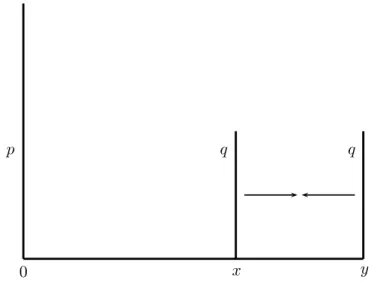
Axiom ER 1. : Consider a population made of three income groups, as shown in Figure 1.1. If the two smaller and closer groups join together at the average of their incomes, polarization increases.
Axiom ER 1considers the effect of reducing local alienation on total polarization. The average distance between the two groups originally at 𝑥 and 𝑦 and the group at 0 does not change. Av-erage alienation does fall, however, because of incomes 𝑥 and 𝑦 moving closer. Axiom ER1says that the effect of increased identification of the two groups to the right dominates the reduction of alienation. It also implies that the polarization index should be concave in alienation: the effect of the increased alienation between those at incomes 0 and (initial) 𝑥 dominates the effect of the lower alienation between those at 0 and (initial) 𝑦.
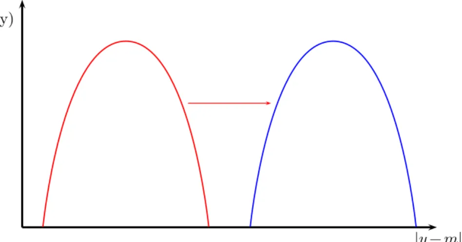
Axiom ER 2. : Consider a population made of three income groups, as shown in Figure 1.2. If 𝑥 moves to the right towards 𝑦, polarization increases.
Axiom ER2involves two changes in alienation. The first one is a fall in alienation between those at 𝑥 and those at 𝑦. The second is an increase in alienation between those at 0 and those at 𝑥. Axiom ER 2says that the greater proximity of 𝑥 and 𝑦 should increase polarization. Axiom ER
2 also implies that the index should be convex in alienation. The combinations of Axioms ER1
Figure 1.1: Merging two relatively small and close groups at the average of their incomes increases polarization.
0 𝑥 𝑦
𝑝 𝑞 𝑞
Note: there are 𝑝 individuals at income 0, 𝑞 individuals at income 𝑥 and 𝑞 individuals at income 𝑦. The incomes of the 𝑞 + 𝑞 individuals are changed to (𝑥 + 𝑦)/2.
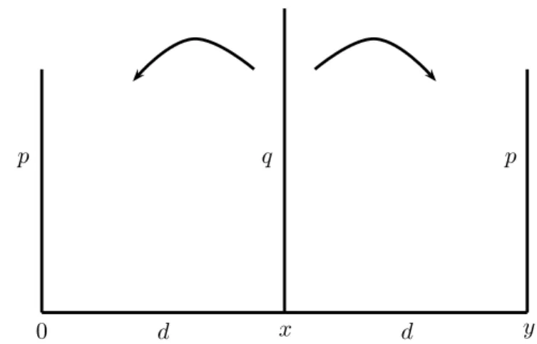
Axiom ER 3. : Any new distribution formed by shifting population mass from a central mass of size 𝑞 equally to two lateral masses each of size 𝑝 and equally distant away from the central mass increases polarization; seeFigure 1.3for an illustration.
Axiom ER 3says that absorption (or disappearance) of the middle class into richer and poorer classes should increase polarization. It puts a bound on the relative importance of identification in the measurement of polarization: the effect of the fall in identification felt by middle-class individuals located at 𝑥 in Figure 1.3 should not be too strong in relation to the effect of the increase in identification felt by those individuals on each side of the middle class.
Esteban and Ray(1994) then shows that this framework implies a particular form forEquation
(1.1):
Theorem 1.4.1. : A class of polarization measure satisfies condition 𝐻 and the three axioms ER
1, ER 2 and ER3 above if and only ifEquation (1.1) has the form: 𝐸𝑅(𝛼, 𝐅) = 𝐾 𝑛 ∑ 𝑖=1 𝑛 ∑ 𝑗=1 𝑛1+𝛼 𝑖 𝑛𝑗|𝑦𝑖− 𝑦𝑗| (1.2)
where 𝐾 > 0 is a normalization constant and 𝛼 ∈ (0, 1.6], and if therefore 𝑇 {𝐼(𝑛𝑖), 𝑎[𝛿(𝑦𝑖, 𝑦𝑗)]} =
𝑛𝛼
Figure 1.2: Moving 𝑥 towards 𝑦 increases polarization.
0 𝑥 𝑦
𝑝 𝑞 𝑟
Note: there are 𝑝 individuals at income 0, 𝑞 individuals at income 𝑥 and 𝑟 individuals at income 𝑦. Incomes 𝑥 is moved upwards.
A few remarks may be useful. There are only two degrees of freedom in Equation (1.2), each based on 𝐾 and 𝛼. 𝐾 is a simple multiplicative constant that has no effect on the ordering of distributions. 𝛼 reflects the relative importance of identification and alienation, commonly referred to as a parameter of “polarization aversion”. The polarization measure bears resemblance to the Gini coefficient. Aside from the fact that Equation (1.2) uses the logarithm of incomes (see below), it would equal the Gini if 𝛼 were equal to zero. The fact that 𝛼 can exceed zero distinguishes income polarization and inequality. The larger the value of 𝛼, the greater the departure from inequality measurement since the greater the departure of Equation (1.2)from the pure consideration of income distances.
In the formulation of Esteban and Ray (1994), 𝑦𝑘 in Equation (1.2) is taken to be the log of income (or the log of the relevant cardinal variable). One justification is that individuals may be sensitive to percentage differences in income and not to absolute differences in them. Another justification is that the measure Equation (1.2) is then invariant to proportional changes in all incomes. The use of income logarithms makes, however, the polarization measure to be non-comparable with the Gini index even when the 𝛼 parameter is set to zero. Furthermore, 𝐾 = 𝜇−1
could be used in such a way as to makeEquation (1.2)invariant to proportional changes and all incomes, when incomes and not income logarithms are used in the formula.
Figure 1.3: Absorption of the middle class into richer and poorer classes increases polarization.
0 𝑑 𝑥 𝑑 𝑦
𝑝 𝑞 𝑝
Note: there are 𝑝 individuals at income 0, 𝑞 individuals at income 𝑥 and 𝑝 individuals at income 𝑦 = 2𝑥 = 2𝑑. Part of the 𝑞 individuals at 𝑥 are shifted equally to 0 and 𝑦.
1.4.2 Continuous income polarization
The discrete formula inEquation (1.2)provides an index whose application to indicators of wel-fare that are commonly continuous (such as income) raises difficulties. First, both the number and the location of income groups are assumed to be (potentially arbitrarily) set/pre-identified. Second, a marginal change in the value of 𝑦 for some individuals may lead to a non-marginal change in the polarization index (as when a small change in income changes group sizes dis-cretely), a discontinuity that would seem regrettable.
Duclos et al. (2004) [DER] addresses both of these issues in a framework that is reminiscent
of Esteban and Ray (1994) in surface, but with differences at a deeper level. DER postulates
that their polarization index should be proportional to the sum of all effective antagonisms in a continuous distribution,
𝐷𝐸𝑅 = ∫ ∫ 𝑇 [𝑓(𝑥), |𝑥 − 𝑦|]𝑓(𝑥)𝑓(𝑦)𝑑𝑥 𝑑𝑦, (1.3) where 𝑓(𝑥) is the (un-normalized) density function — capturing identification — and |𝑥 − 𝑦| = 𝑎 is the distance between individuals of income 𝑥 and 𝑦 — capturing alienation. The antagonism function 𝑇 (𝐼, 𝑎) is increasing in its second argument and 𝑇 (𝐼, 0) = 𝑇 (0, 𝑎) = 0.
A functional expression for Equation (1.3) is characterized through the formulation of axioms that, though analogous to those of Esteban and Ray (1994), differ in that the income space is continuous. The domains of the axioms are primarily the union of one or more “basic densities”. These densities are symmetric, unimodal, normalized by population size, and have a compact support. For 0 < 𝑟 < 1, a 𝑟-squeeze of a density function is defined as a transformation of the form 𝑓𝑟(𝑥) =1
𝑟𝑓 [𝑥−(1−𝑟)𝜇𝑟 ] such that 𝑓𝑟 is a density. The transformation leaves the mean of
the distribution unchanged but reduces its standard deviation by a factor 1 − 𝑟. The first axiom considers the polarization impact of squeezing basic densities — the first one locally and the second one for two densities, each located on either side of a middle class. These two axioms make it possible to define the role of identification in the antagonism function 𝑇 (𝐼, 𝑎). The third axiom considers the impact of changes in alienation and thus the role of 𝑎 in 𝑇 (𝐼, 𝑎). The fourth axiom is a population invariance axiom.
Axiom DER 1. : A squeeze of a distribution made of only one basic density (as shown in
Figure 1.4) does not increase polarization.
Alienation diminishes and identification rises following this squeeze; the impact on polarization of greater identification is nevertheless offset by the impact of a decline in alienation. This effectively limits the parameter 𝛼 (that will be introduced below, seeEquation (1.4), and which is the analogue of the 𝛼 of the discrete formulation of Equation (1.2)) to be no greater than one, since Axiom DER 1 says that polarization should not depart excessively from inequality measurement.
Figure 1.4: A squeeze of a basic density does not increase polarization
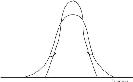
Axiom DER 2. : If the distribution of a symmetric density has three poles (see Figure1.5), then a squeeze of the outer poles does not decrease polarization.
Figure 1.5: A double squeeze cannot reduce polarization
Income The decline of inter-group alienation in the outer poles is counterbalanced by the rise of iden-tification. Axiom DER 2 is the “defining” axiom of polarization: it differentiates polarization from inequality. It also puts a lower bound on the parameter 𝛼 in Equation (1.4): it should not lie below 0.25 for the fall in local alienation (the alienation within each extreme group) to be outweighed by the increase in identification. The axiom also implies that the polarization index should be concave in alienation — for the fall in larger alienation values (the more extreme distances from the middle fall following the squeeze) not to have too large an impact on total polarization.
Axiom DER 3. : If a symmetric density has four poles and if each of the two middle poles shifts to the nearer outer pole, as in Figure 1.6, then polarization must go up.
Figure 1.6 shows a fall in local alienation combined with an increase in larger alienation values (an increase in the larger distances between groups). This implies that polarization should be weakly convex is alienation; the effect of a fall in smaller distances should be outweighed by a similarly-sized increase in the value of larger distances. Axioms DER 2 and 3 imply that polarization should be linear in alienation.
Axiom DER 4. : If the polarization index for one distribution is higher than for another one, then it remains higher when both populations are identically scaled.
Figure 1.6: A symmetric outward slide must raise polarization
Income This axiom states that polarization orderings should be invariant to population size. It plays a role similar to Condition H on page 14 above for discrete income polarization. It links iden-tification and polarization through a constant elasticity function in Equation (1.4). DER then shows that:
Theorem 1.4.2. : The index in Equation (1.3) satisfies axioms DER 1 to 4 if and only if it is proportional to:
𝐷𝐸𝑅(𝛼) = ∫ ∫ 𝑓(𝑥)1+𝛼𝑓(𝑦)|𝑥 − 𝑦|𝑑𝑥𝑑𝑦 (1.4)
for 𝛼 ∈ [0.25 1], and if therefore 𝑇 [𝑓(𝑥), |𝑥 − 𝑦|] = 𝑓(𝑥)𝛼|𝑥 − 𝑦|.
Making polarization invariant to proportional changes in all incomes can be done by multiplying 𝐷𝐸𝑅(𝛼) by 𝜇𝛼−1. For 𝛼 = 0, the measure would be equivalent to the Gini coefficient. Note,
however, thatTheorem (1.4.2)excludes the Gini index: the Gini index would indeed fall following the squeeze of Figure 1.4, which would violate Axiom DER 2.
The 𝐷𝐸𝑅(𝛼) polarization index can be decomposed into identification and alienation compo-nents. For a particular value of 𝛼, average 𝛼-identification can be expressed as
𝜄𝛼≡ ∫ 𝑓(𝑦)𝛼𝑑𝐹 (𝑦) = ∫ 𝑓(𝑦)1+𝛼𝑑𝑦. (1.5)
The average alienation felt by an individual with income 𝑦 is given by 𝑎(𝑦) = ∫ |𝑦 − 𝑥|𝑑𝐹 (𝑥), and the overall average alienation is thus 𝑎 = ∫ 𝑎(𝑦)𝑑𝐹 (𝑦) = ∫ ∫ |𝑦 − 𝑥|𝑑𝐹 (𝑥)𝑑𝐹 (𝑦), which is propor-tional to the Gini index. Let 𝜌𝑖,𝑎= cov[𝑓(𝑦)𝜄 𝛼,𝑎(𝑦)]
and alienation. Then, 𝐷𝐸𝑅(𝛼) = 𝜄𝛼𝑎[1 + 𝜌𝑖,𝑎]. Ceteris paribus, this means that greater multi-modality in the density is likely to translate into greater 𝜄𝛼 and into greater polarization — this effect becoming stronger when 𝛼 is larger. Greater inequality and thus greater average alienation 𝑎 will also mean greater polarization. Finally, a greater covariance 𝜌𝑖,𝑎 between identification and alienation will raise polarization.
1.4.3 Discrete income polarization with endogenous grouping
The 𝐷𝐸𝑅(𝛼) index effectively sets the number of possible income groups to infinity. Each group displays perfect internal homogeneity, being associated with one and only one income level. That removes the need for selecting either the number or the position of income groups.
We might, however, think of measuring income polarization on the basis of a finite and pre-specified number of income groups and select their position in order to maximize internal group homogeneity. Choosing positions to maximize internal homogeneity has the advantage of max-imizing local identification and minmax-imizing local alienation — but since individuals in a given group do not all have the same income with discrete income groupings, there will necessarily remain internal heterogeneity even after such an optimization procedure.
Such an approach is used byEsteban et al. (2007) on the Esteban and Ray (1994) index, using a continuous variable such as income and specifying the number of income groups to be used but not their precise location. Clustering into a finite number of classes introduces errors in the measurement of continuous income polarization. This clustering introduces an approximation error 𝜖(𝐅). The greater the error, the greater the level of internal heterogeneity, the lower the level of internal identification, the greater the level of local alienation, and the greater the likelihood of a bias in using 𝐸𝑅(𝛼, 𝐅) as an index of continuous income polarization. An “extended” polarization index that attempts to correct for such biases is given by:
𝐸𝐺𝑅(𝛼, 𝜎, 𝐅) = 𝐸𝑅(𝛼, 𝐅) − 𝜎𝜖(𝐅), (1.6) where 𝛼 is the usual polarization sensitivity parameter and 𝜎 is a parameter that weights the measurement error. The approximation error is specified as
𝜖(𝐅) = ∑ 𝑖 ∫ 𝑥 ∫ 𝑦 |𝑥 − 𝑦|𝑑𝐹𝑖(𝑥) 𝑑𝐹𝑖(𝑦) (1.7) and the problem is set to minimize 𝜖(𝐅) for a given number 𝑛 of groups. From Equation (1.7), it can be seen that it is equivalent to minimizing the sum of the within-group Gini indices or, alternatively, to minimizing the sum of within-group alienation. The solution is denoted by 𝐅∗,
with
where 𝐺𝐵(.) is between-group Gini coefficient of 𝐅∗. TheEsteban et al. (2007) index is then
𝐸𝐺𝑅(𝛼, 𝜎, 𝐅∗) = 𝐸𝑅(𝛼, 𝐅∗) − 𝜎𝐺𝐵(𝐅∗). (1.9)
Note that 𝜎𝐺𝐵(𝐅∗) is originally meant to capture the effect of one error, the overestimation
by 𝐸𝑅(𝛼, 𝐅∗) of income identification in a context in which incomes are artificially grouped.
Another error also exists, however, and comes from the underestimation by 𝐸𝑅(𝛼, 𝐅∗) of income
alienation in a context in which local alienation is removed through a discrete formation of income groups. The true approximation error of the Esteban and Ray (1994) is therefore quite complicated, and should attempt in particular to account both for the identification and for the alienation errors of grouping individuals. The formulation of the error should also be consistent with the special form taken by the Esteban and Ray (1994) index; Equation (1.9) takes the awkward shape of a difference between non-comparable functions whenever 𝛼 is different from zero.
An example of a difficulty created by the form of Equation (1.9) is noted in Lasso de la Vega
and Urrutia(2006); theEsteban et al.(2007) measure may fall when groups move farther away
from each other because identification errors may increase when this happens, with a resulting fall in Equation (1.9). The alternative index proposed in Lasso de la Vega and Urrutia (2006) is given by 𝐶𝑀 (𝛼, 𝛽, 𝐅) = 𝐾 ∑ 𝑖 ∑ 𝑗 𝜋𝑖𝜋𝑗𝜋𝛼 𝑖(1 − 𝐺𝑖)𝛽| 𝑙𝑛 𝜇𝑖− 𝑙𝑛 𝜇𝑗| (1.10)
where 𝛽 ≥ 0 is the degree of sensitivity towards group cohesion, 𝐺𝑖 the Gini coefficient of group 𝑖, 𝐾 is a normalization constant and 1 − 𝐺𝑖 the Gini equality coefficient of group 𝑖. The new identification term for each member of group 𝑖 is thus 𝜋𝛼
𝑖 (1 − 𝐺𝑖)𝛽, a term that decreases with
group Gini. (One could also think of maximizing 𝐶𝑀 (𝛼, 𝛽, 𝐅) over a fixed number of groups, in the spirit of the Esteban et al. (2007) index, yielding 𝐶𝑀 (𝛼, 𝛽, 𝐅∗).) As for Equation (1.9),
Equation (1.10) does not explicitly account for the dual nature of the identification/alienation approximation error.
1.5 Bi-polarization
1.5.1 Measures of the size of the middle class
Income polarization captures the existence and the importance of an arbitrary number of income poles; bi-polarization measures the extent to which a population is divided into two separate groups. An important motivation for developing the concept of bi-polarization has been the