Radars in Transport Applications

Science Arts & Métiers (SAM)

is an open access repository that collects the work of Arts et Métiers Institute of Technology researchers and makes it freely available over the web where possible.

This is an author-deposited version published in: https://sam.ensam.eu

Handle ID: .http://hdl.handle.net/10985/18620

To cite this version :

Rubén IBÁÑEZ PINILLO, Francisco CHINESTA, Emmanuelle ABISSET-CHAVANNE, Erik ABENIUS, Antonio HUERTA - Radars in Transport Applications - 2020

Any correspondence concerning this service should be sent to the repository Administrator : [email protected]

Chapter 12

Radars in Transport Applications

Rubén Ibáñez Pinillo, Francisco Chinesta, Emmanuelle Abisset-Chavanne, Erik Abenius and Antonio Huerta

Abstract In the recent years, automotive car industry is evolving towards a new

generation of autonomous vehicles, where decision making is not fully perform by the driver but it partially relies on the technology of the car itself. Indeed, a CPU inside the car will process all information coming from the sensors, distinguishing different scenarios appearing in the real life and ultimately allowing decision making. Since the CPU will be confronted with plenty of information, tools like machine learning or big-data analysis will be a useful ally to separate big-data from information. These existing machine learning techniques, such as kernel Principal Component Analysis (k-PCA), Locally Linear Embedding (LLE) among many other techniques, are useful to unveil the latent parameters defining a given scenario. Indeed, these algorithms have been already used to perform real-time classification of signals appearing throughout the road. Selecting the modeling of the electromagnetic response of the radar plays an important role to achieve real time constraints. Even though Helmholtz equation represents accurately the physics, the computational cost of such simulation is not affordable for real-time applications due to high radar operating frequencies, resulting into a very fine finite element mesh. On the other hand, far field approaches are not so

R. Ibáñez Pinillo (

B

École Centrale de Nantes, Nantes, France e-mail:[email protected]

F. Chinesta

ENSAM, ParisTech 151, bld. de l’Hôpital, F-75013 Paris, France e-mail:[email protected]

E. Abisset-Chavanne

École Centrale de Nantes, ESI GROUP Chair, High Performance Computing Institute, 1 Rue de la Noe, 44300 Nantes, France

e-mail:[email protected] E. Abenius

ESI Group, Sjöängvägen 15, SE-19272 Stockholm, Sweden e-mail:[email protected]

A. Huerta

Universitat Politècnica de Catalunya, Barcelona, Spain e-mail:[email protected]

accurate when the objects are very close due to plane wave assumption. In the first part of this work, the Geometrical Optics method is investigated in this work as a possible route to fulfill both real-time and accuracy constraints. The main hypothesis under such model is that waves are treated as straight lines constrained to optical reflection laws. Therefore, there is no need to mesh the interior of the domain. However, the accuracy of such approach is compromised when the size of the objects inside the domain are comparable to the wave lengths or in the vicinity of angular points. The second part is mainly focused on of the application of manifold learning and big data analysis into a data set of precomputed scenarios. Indeed, the identification of an unknown scenario from electromagnetic signals is purchased. Nevertheless, current research lines are devoted to give an answer to questions such as how many receptors do we need to identify unequivocally the scenario, where to locate the receptors, or which parts of the scenario have a negligible impact in the electromagnetic response.

Keywords ADAS

·

·

·

12.1 Introduction

Automotive car industry is moving towards a new generation of autonomous vehicles, where the driver is not the main responsible of decision making but the technology of the car itself. Indeed, a CPU inside the car will process all information coming from the sensors, allowing to distinguish different scenarios appearing in the real life. Since the CPU will be confronted with plenty of information, tools like machine learning or big-data analysis will be useful to separate data from information. Thus, Sect.12.2 provides an state of art of existing machine learning techniques Roweis and Saul [3]; Scholkopf et al. [4]; Lee and Verleysen [1] which are meant to be useful when unveiling the latent parameters definining a given scenario.

Regarding the modeling of the electromagnetic response of the radar, even though Helmholtz equation represents accurately the physics, the computational cost of such simulation is not affordable for real-time applications due to high radar operating frequencies, resulting into a very fine finite element mesh. On the other hand, far field approaches are not so accurate when the objects are very close due to plane wave assumption. That is the reason why, the Geometrical Optics method is investigated in Sect.12.3to fulfill both real-time and accuracy constraints. The main hypothesis under such model is that waves are treated as straight lines constrained to optical reflection laws. Therefore, there is no need to mesh the interior of the domain. How-ever, the accuracy such approach is compromised when the size of the objects inside the domain are comparable to the wave lengths or in the vicinity of angular points.

Section12.4consists of the application of manifold learning and big data analysis into a data set of precomputed scenarios. Indeed, the identification of an unknown scenario from electromagnetic signals is purchased. Nevertheless, in our future work we will try to give an answer to questions such as how many receptors do we need to identify unequivocally the scenario, where to locate the receptors, or which parts of the scenario have a negligible impact in the electromagnetic response.

12.2

State of Art Manifold Learning

In this section, and for the sake of completeness, two widely employed manifold learning techniques are revisited: Principal Component Analysis (PCA) and the Locally Linear Embedding (LLE) Roweis and Saul [3]; Lopez et al. [2].

12.2.1 Principal Component Analysis

Let us consider D observed variables defining the vector y_{∈ R}D_{. These are}

com-monly referred as the snapshots of the system: nodal values of the essential field throughout time in usual finite element modeling. We assume that these variables are therefore not uncorrelated and, notably, that there exists a linear transformation W defining the vector ξ _{∈ R}d_{, where d < D represents the unknown so-called latent}

variables, according to

y = Wξ. (12.1)

The transformation W, D_{× d, is assumed to verify the orthogonality condition}

WT_{W = I}

d, where Idrepresents the d× d-identity matrix (WWTis not necessarily

ID). The existence of such a transformation is precisely at the origin of PCA methods.

We assume the existence of M different snapshots y₁, . . . ,y_M, that can be stored in the columns of the D_{× M matrix Y. The associated d × M reduced matrix !} contains the associated vectors ξ_i, i _{= 1, . . . , M.}

We assume that both observed and latent variables are centered, that is ! "M

i₌₁yi = 0

"M

i₌₁ξi = 0

. (12.2)

If it is not the case, prior to proceed, observed variables must be centered by removing the expectation of E_{{y} to each observation y}i, i = 1, . . . , M. Since the

exact expectation is unknown, one commonly accepted procedure is to substitute it by the sample mean.

PCA is able to calculate both d—the necessary number of members in the basis of the reduced-order subspace—and the transformation matrix W. PCA proceeds by guaranteeing maximal preserved variance and decorrelation in the latent variable set ξ. From a statistical point of view, therefore, it can be assumed that the latent variables in ξ are uncorrelated (no linear dependencies among them) or mutually orthogonal, thus constituting a basis. In practice, this means that the covariance matrix of ξ, defined as

Cξξ = E{!!T}, (12.3)

However, the observed variables are expected to be correlated. The goal of PCA is then to extract the d uncorrelated latent variables in υ, according to

Cyy = E{YYT} = E{W!!TWT} = WE{!!T}WT = WCξξWT, (12.4)

that by pre-multiplying and post-multiplying by WT_{and W respectively, and taking}

into account that WT_{W = I, leads to:}

C_{ξξ = W}T_C

yyW. (12.5)

The covariance matrix Cyy can then be factorized by applying the singular value

decomposition,

Cyy = V"VT, (12.6)

with V containing the orthonormal eigenvectors and " the diagonal matrix containing the eigenvalues assumed in descending order.

Substituting the factorized expression of the covariance matrix (12.2) into Eq. (12.1) it results

C_{ξξ = W}T_V"VT_{W. (12.7)}

This equality holds only when the d columns of W are taken collinear with d columns of V. If the PCA model is fully respected, then only the first d eigenvalues in " are strictly larger than zero; the other ones are zero.

The eigenvectors associated with these d nonzero eigenvalues must be kept:

W = VID_×d, (12.8)

yielding

C_{ξξ = I}d_×D"ID_×d. (12.9)

This shows that the eigenvalues in " correspond to the variances of the latent variables (the diagonal entries of C_ξξ).

In real situations, some noise may corrupt the observed variables. As a conse-quence, all eigenvalues of C_ξξare larger than zero, and the choice of d columns in V becomes more difficult. Assuming that the latent variables have larger variances than the noise, it suffices to choose the eigenvectors associated with the largest eigenval-ues. This is the common practice in finite element model order reduction procedures. A number of columns of V are kept so as to preserve a chosen amount of the energy of the system.

From a geometrical point of view, the columns of V indicate the directions in_RD

that span the subspace of the latent variables ξ. The name PCA then arises naturally from the fact of keeping the components associated with the largest variance.

PCA constitutes a polyvalent method, developed, discovered and re-discovered many times in different branches of applied science and engineering. It deter-mines data dimensionality, builds an embedding accordingly, and extracts the latent

Fig. 12.1 Geometrical interpretation of PCA

Fig. 12.2 PCA limits in presence of strongly-nonlinear manifolds

variables. However, PCA is still based upon one critical assumption: the linear depen-dency expressed by Eq. (12.1) between observed and latent variables (in other words, between the reduced-order and full-order models).

From a geometrical point of view, the columns of V indicate the directions in RD _{that span the subspace of the latent variables. We illustrate this interpretation}

in Fig.12.1 where at left we can appreciate points that apparently belongs to _R2_,

however, it is easy to see that all these points belong to a slow one-dimensional manifold. PCA find an alternative coordinate system given by V (axes in red) in which all these points are described from a single coordinate.

Frequently, latent variables posses a manifold structure, and therefore it simply does not exist a basis able to construct a projection such as that in Eq. (12.1). This is the case, for instance, in non-linear, large strain solid dynamics. Nonlinear methods are often more powerful than linear ones, because the connection between the latent variables and the observed ones may be much richer than a simple matrix multipli-cation. This situation is sketched in Fig.12.2where it can be noticed that no-rotation allows to extract the one-dimensional slow manifold. Thus, PCA seems informing that the different points belongs to a two-dimensional space, with the risk of con-cluding that the closest point (using the 2D euclidean distance) to the red point is in fact one that is very far from it when using the more appropriate geodesic distance on the one-dimensional slow manifold. Thus, the extraction of the slow manifold is compulsory and PCA is unable to accomplish the job.

Local-PCA-lPCA—applies standard PCA locally, that is, at each data-point and its closest neighbors. It is sketched in Fig.12.3. The main issue related to its practical

Fig. 12.3 Sketch of

local-PCA

implementation is the alignment of the local bases unfolding the slow manifold, as discussed in many papers, e.g. Zhang and Zha [5].

12.2.2 Locally Linear Embedding

We consider the different points yi ∈ RD, i = 1, . . . , M, and proceed in two steps:

1. Each point yi, i = 1, . . . , M is linearly interpolated from its K nearest neighbors

(“locally linear”). In principle K should be greater that the expected dimension

d of the underlying manifold and the neighbors should be close enough so as to ensure the validity of linear approximation. In general, a small but enough number of neighbors K and a large-enough sampling M ensures a satisfactory reconstruction. For each point yi we can write the locally linear data

reconstruc-tion as:

yi =

#

j∈Si

Wi jyj, (12.10)

where Wi j are the unknown weights and Si the set of the K -nearest neighbors

of yi. If we perform this locally linear interpolation for every data point in the

high dimensional space, the set of weights that best approximates the manifold structure of the data will be obtained by minimizing the functional

F(W) = M # i=1 $ $ $ $ $ $yi − M # j=1 Wi jyj $ $ $ $ $ $ 2 , (12.11)

where Wi j is zero if yj does not belong to the set of K -nearest neighbors of yi.

2. We assume now that each linear patch around yi,∀i, is mapped onto a lower

dimensional embedding space of dimension d _{≪ D. To maintain the} neigh-borhood structure of the set weights are assumed to remain unchanged in the

low-dimensional, embedding space. The problem thus becomes the determina-tion of the coordinates of each point yi in the low dimensional embedding space,

ξi ∈ Rd. For this purpose a new functional G is introduced, that depends on the

searched coordinates ξ1, . . . ,ξM G(ξ1, . . . ,ξM)= M # i=1 $ $ $ $ $ $ξi − M # j=1 Wi jξj $ $ $ $ $ $ 2 , (12.12)

where now the weights are known and the reduced coordinates ξi are unknown.

The minimization of functional G results in a M × M eigenvalue problem whose

d-bottom non-zero eigenvalues define the set of orthogonal coordinates in which the manifold is mapped.

It is important to note that functional G(ξ1, . . . ,ξM), with the different

coor-dinates ξi already calculated as just described, offers an error estimator on the

locally linear embedding capacity, and even a local estimator can be derived by considering E(ξi)= $ $ $ $ $ $ξi − M # j₌₁ Wi jξj $ $ $ $ $ $. (12.13)

Thus, if we consider the introduction of a new point ξ in the embedding space_Rd_after

identifying its neighbors set S(ξ) and calculating the locally linear approximation weights, we can come back to_RD _{and reconstruct y from its neighbors y}

i, i ∈ S(ξ).

12.3 Geometrical Optics

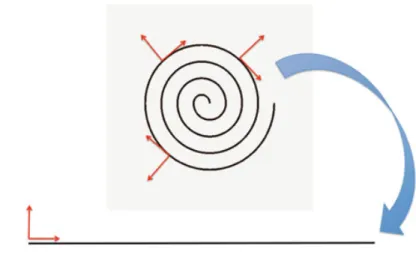
In this part, the basic concepts behind geometrical optics phylosophy are revisited. This approach combines optical reflection plus a balance of energy based on a loss of energy each time a reflection is produced. Figure12.4 represents how a laser is reflected inside a closed surface (∂Ω), the reflections will stop when the energy carried by the ray becomes zero. Each time a reflection occurs, a given amount of energy is lost according to the absorption coefficient of the surface. Therefore, if a given laser is thrown with a initial energy (Eext) from a initial point (x0), such

energy will be distributed along the surface (Eint) according to the geometry and the

absorption coefficient distribution, as shown in Eq. (12.14).

Eext(x0)= Eint(x), x ∈ ∂Ω (12.14)

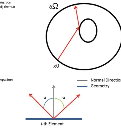
Hence, our main goal is to build a system of equations able to give us the spatial distribution of the absorbed energy Eint(x) for a given source located at the position x0with an intensity that may depend on the angle of departure (θd), so Eext(x0,αd).

Figure12.5shows the convention for the angle of departure, it is measured from the local normal direction. A counterclockwise rotation of the normal direction will

Fig. 12.4 Closed surface

(∂Ω), laser ray (red) thrown from x0

Fig. 12.5 Angle departure

criterium

generate a positive angle of rotation, whereas a clockwise rotation will provide a negative angle. Indeed, all angular measurements will remain local since they depend on the local normal direction.

When discretizing the element source x0 into D-angular directions where the

received energy could be stored, it will give an energy vector whose size is_[D].

Es = ⎡ ⎢ ⎣ Eα1 x0 .. . EαD x0 ⎤ ⎥ ⎦ (12.15)

where E_xα j₀ is the energy absorbed in x0, with an angle of arrival αj.

The balance of energy between the energy going out from the source (x0) and the

energy coming back to the same point, could be written as a system of Eq. (12.16).

Es = Mf (12.16)

where (i, j) component of the matrix M is the energy coming back to the source with an discretized arrival angle αa = i∆α, which has been thrown from an angle

Fig. 12.6 Balance of energy

for one ray

of departure αd = j∆α and f is the external energy of the source. The size of M is

the angular discretization points (_{[D × D]).}

Figure12.6exemplifies how a column of matrix M is constructed. Imagine that the source has five discretized angles. Equation (12.17) describes the balance between a source located at x0 with angle of departure α4 and the received energy at the same

element with an angle α2. The r coefficient takes into account the energy absorptions

due to reflection that the ray has suffered till it arrives to the same departure point.

Eα4

ext = r Exα02 (12.17)

If the same process is repeated for any possible angle of departure, the system of equations (12.16) is obtained. Moreover, any possible source could be described as the addition of unitary impulsional sources multiplied by their magnitude since the problem is linear. (i.e. the absorption coefficient does not depend on the magnitude of the incident wave.)

It is important to recall that all reflections that occur while the ray is traveling along the domain are analytical, thus the only kind of discretization error is the angular discretization of the source. That is the reason why, a convergence analysis in terms of angular discretization is crucial in this case.

12.3.1 Convergence Results

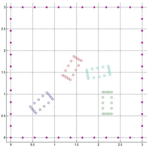
Figure12.7shows the domain where the algorithm is tested. There are four obstacles which have an absorption coefficient of 0.5, whereas the external wall has an

absorp-Fig. 12.7 Scenario used to test the convergence results

tion coefficient of 1. The source is located at the middle point of the south external wall.

Equation (12.18) defines the total energy coming back to the radar from the source, it is a constant scalar quantity. For this convergence analysis, the source and the receptor will be located at the same region.

ET = + π 2 −π 2 + π 2 −π 2 E(αd,αa)dαddαa (12.18)

where αd and αa are the departure and arrival angles, respectively.

On the other hand, quantities giving a glimpse of directional energy such as Eqs. (12.19), (12.20), (12.21) are interesting, since the total energy (ET) could be a

poor descriptor sometimes.

ED(αd)= + π 2 −π 2 E(αd,αa)dαa (12.19) EA(αa)= + π 2 −π 2 E(αd,αa)dαd (12.20)

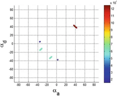
Fig. 12.8 Energy coming back to the radar as a function of departure and arrival angles, ED A

ED A(αd,αa)= E(αd,αa) (12.21)

where EDis the energy coming back to the radar as a function of the departure angle,

EAis the energy coming back to the radar as a function of the arrival angle and ED A

is the energy coming back to the radar as a function of both arrival or departure angles.

Figure12.8shows the ED A function for the tested scenario. As it can be seen in

the ED A, there is a primal reflection occuring at an angle of 40◦, caused by the blue

car. Furthermore, there are more secondary reflections coming from the interaction with the other cars. Functional ED A is the indicator that contains more information

since it keeps track of both departure and arrival angles. Indeed, if we have ED A,

building the other two indicators is just a mere integration into a given direction. Equation (12.22) defines the energetic error. Where EH

T is the total energy coming

back to the radar for the most refined solution and EL

T is the total energy coming

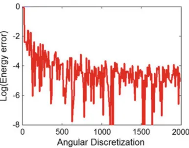
back to the radar for a less refined solution. E = ||E H T − ETL|| EH T (12.22) Figure12.9 shows the energetic error in logarithmic scale varying the angular discretization. The reference solution is constructed with 8000 discretized angles. As it can be seen, there is a fast convergence at the beginning. However, beyond 500 discretized angles, the solution starts to saturate, giving a relatively slow convergence

Fig. 12.9 Convergence

analysis in terms of the angular discretization

slope. It is important to notice that the solution is already quite good since we are in 4 digits of accuracy.

12.3.2 Black-Boxing the Scenario

The convergence results shown so far are based on relatively easy obstacles. Indeed, only four straight sides were required to replicate a square-like obstacle. Let’s imagine for a single moment that our object in the scenario is hard to replicate i.e. a real car, an extrange pedestrian, etc. Therefore, a lot of elements will be required to represent accurately the real geometry of the obstacle, compromising the computational cost of the algorithm.

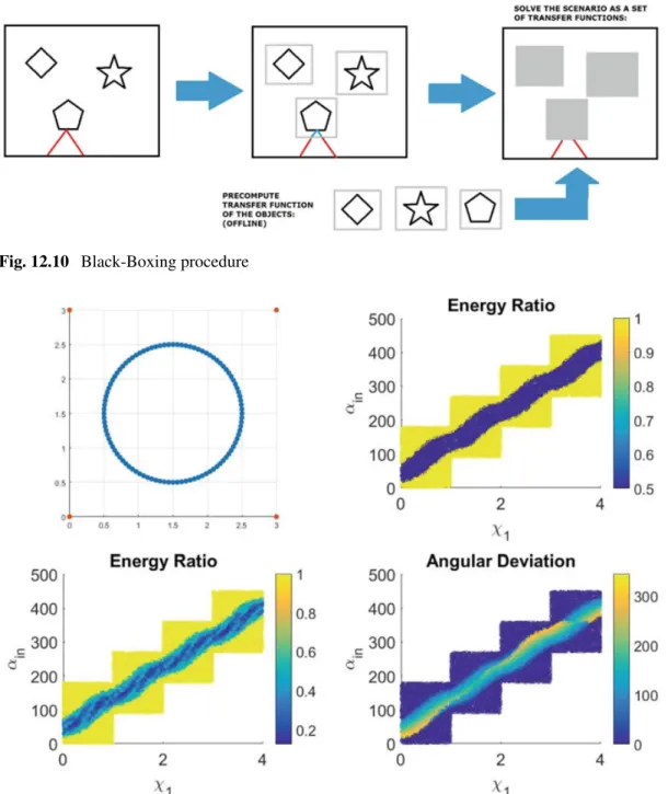
Black-Boxing consists of computing the response of an obstacle off-line, gen-erating a library with all possible objects and defining a transfer function for each one of them. Then, if we know the obstacles inside our scenario, we will not have to reproduce the exact geometry but replace it with a Black-Box having a transfer function characteristic of the object inside. Figure12.10schematizes such procedure. This transfer function consists of knowing three variables: the ratio of dissipated energy and both the location and angular direction of the outgoing ray. These three ingredients are functions of both the location and angular direction of the incoming ray. Figure12.11 shows how a circle is black-boxed. As it can be seen, only two parameter, the box arclength (χ) and the income angular direction (αin), suffices to

characterize the three variables defining the transfer function.

Figure12.11shows the transfer function generated with a circle. As it can be seen, the energy ratio subplot gives information of how many reflection the ray has done before going out of the domain. Indeed, the yellow region corresponds with a ray that has not touched the circle, whereas the blue region corresponds with a single reflection since the absorption coefficient was set to 0.5. The other two subplots

Fig. 12.10 Black-Boxing procedure

Fig. 12.11 Three variables definining the circle transfer function of a circle obstacle

making reference to the output length and the angular deviation give information about the location and angular direction of the outgoing ray, respectively.

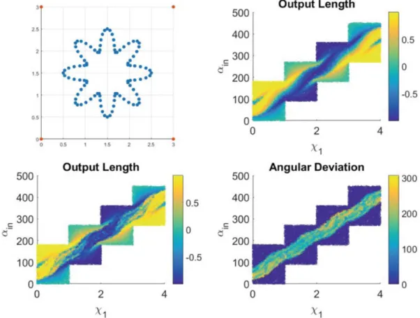
Figure12.12shows the transfer function generated with a star. It is important to note that the energy ratio is smaller than 0.5 since primary, secondary and terciary reflections occurs between the star peaks.

Fig. 12.12 Three variables definining the circle transfer function of a star obstacle

12.4 The Scenario Manifold

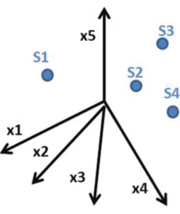
Imagine that a lot of different scenarios are precomputed a priori (off-line) and then they are placed into a dataset as shown in Fig.12.13, which constitutes the scenario manifold MS. Hence, each electromagnetic response (E) depends on the variables to

identify our scenario i.e. geometrical parameters defining both position and orienta-tion of the obstacles. For instance, if a 2D square needs three variables to be identified (i.e. the vector position and the orientation angle), each point in the scenario manifold with N obstacles will be composed of p_{= 3 × N coordinates. Comparing scenarios} involving different number of obstacles is possible by means of a nested representa-tion i.e. defining the maximum number of obstacles and completing the coordinates of a scenario with less obstacles. Furthermore, if angles and positions have to be compared, the angle should be a dimensionalized with respect to a characteristic obstacle length.

Once the scenario manifold is generated, inferring the obstacle positions and orientations knowing a new electromagnetic response constitutes the main industrial interest. Equation (12.23) sets a minimization problem on the data set such that a similar electromagnetic response on the manifold is seeked.

Fig. 12.13 Scenario

manifold

where subindex n makes reference to a new electromagnetic response whose asso-ciated scenario is unknown.

However, the consideration of diverse scenarios may lead to a drastic increment on the cardinality of the parametric space (p). At this point, manifold learning techniques like the ones explained in Sect.12.2will be of crucial importance to define a reduce set of parameters (ξ), where the physics of the problem take place as shown in Eq. (12.24).

argmin,_{||E(α; ξ}n)− E(α; ξi)||- ∀ ξi ∈ MS (12.24)

Another point of critical importance is how to define the electromagnetic response in such a way that the scenario is identified unequivocally. The first inference is done just by knowing the electromagnetic response at one receptor which is located at the same position than the radar, both of them being located at the middle point of the bottom side of the square. Multiple solutions were found to the minimization prob-lem (12.23). Indeed, there are several scenarios that share the same electromagnetic response, being different from a geometrical point of view. Figure12.14(left) shows the a priori unknown scenario (top-left) together with 5 other candidates sharing the same electromagnetic response composed with one receptor. As it can be seen, blue, yellow and purple obstacles varies along the different candidates, whereas the orange location and orientation is consistent along the candidates. Indeed, if a correlation of the obstacles taking into account the different candidates is done, the orange obstacle is the one presenting the most correlated value.

The same procedure is repeated but using three receptors instead of one. All three receptors are placed at the bottom side of the square between point 1 and 2. Once again, the minimization procedure gives several candidates which are shown in Fig.12.14(right). As it can be seen, the position of the orange obstacle is identified properly since this obstacle is the one causing most of the electromagnetic signal. Moreover, the blue obstacle correlation has slightly increased with respect to the

Fig. 12.14 Different candidate scenarios sharing one receptor (left) and three receptor (right)

electromagnetic response

single sensor case. Finally, yellow and purple obstacles remain uncorrelated since they do not cause any electromagnetic variation to the sensors located in the south part of the domain.

12.5 Conclusions

Fast scenario identification is a topic with a huge impact from an industrial point of view. Three different ways of reducing the computational time are being investigated. The first one regards the set of equations employed to solve the problem. Geometrical optics has been investigated as an alternative route to Helmholtz/Maxwell equations to handle high frequency radar signal simulations. The second procedure consists of generating off-line the transfer functions associated to different obstacles, speeding up the on-line computations. The third methodology makes use of manifold learning techniques to extract the relevant information defining the scenario from a electro-magnetic point of view. Questions like the number and position of the sensors to identify in the best possible way the scenario constitutes a current research line.

References

1. Lee J, Verleysen M (2007) Nonlinear dimensionality reduction. Springer, Berlin

2. Lopez E, Gonzalez D, Aguado J, Abisset-Chavanne E, Lebel F, Upadhyay R, Cueto E, Binetruy C, Chinesta F (2016a) Real-time, image-based, simulation of multiscale models based on locally linear embedding. Arch Comput Methods Eng

3. Roweis ST, Saul LK (2000) Nonlinear dimensionality reduction by locally linear embedding. Science 290(5500):2323–2326

4. Scholkopf B, Smola A, Muller K (1999) Kernel principal component analysis. Advances in kernel methods - support vector learning. MIT Press, Cambridge, pp 327–352

5. Zhang Z, Zha H (2004) Principal manifolds and nonlinear dimensionality reduction via tangent space alignement. SIAM J Sci Comput