____________________
* Corresponding author: B 52/3, Chemin des Chevreuils, 1, 4000 Liege, Belgium, +32 (0) 4 366 91 40, +32 (0) 4 366 91 92, [email protected]
ADAPTIVE REMESHING FOR INCREMENTAL FORMING
SIMULATION
Cedric Lequesne
1*, Christophe Henrard
1, Chantal Bouffioux
1, Joost R. Duflou
2,
Anne Marie Habraken
11
University of Liege, ArGEnCo, Liege, Belgium
2Katholieke Universiteit Leuven, PMA, Leuven, Belgium
ABSTRACT:
Incremental forming of aluminium sheets has been modelled by finite element simulations. However the computation time was prohibitive because the tool deforms every part of the sheet and the mesh along the tool path must be very fine. Therefore, an adaptive remeshing method has been developed. The elements that are close to the tool are divided into smaller elements in order to have a fine mesh where high deformations occur. Consequently, some new nodes become inconsistent with the non-refined neighbouring elements. To overcome that problem, their displacements are constrained, i.e. dependent on their master nodes displacements. The data concerning these new nodes and elements are stored in a linked list, which is a fundamental data structure. It consists of a sequence of cells, each containing data fields and a pointer towards the next cell. The goal of this article is to explain the developments performed in the finite element code, to validate the adaptive remeshing technique and to measure its efficiency using the line test simulation. During this test, which is a simple incremental forming test, a clamped sheet is deformed by a spherical tool moving along a linear path.KEYWORDS:
Remeshing, Finite Element Simulation, Incremental Forming1
INTRODUCTION
Single point incremental forming (SPIF) is a sheet metal forming process that is very appropriate for rapid prototyping because it does not require any dedicated dies or punches to form a complex shape. Instead, it uses a standard smooth-end tool mounted on a numerically controlled multi-axis milling machine. The tool follows a complex tool-path and progressively deforms a clamped sheet into its desired shape ([1], [2]).
Simulating this process is a complex task. First, the tool diameter is small compared to the size of the metal sheet. Moreover, during its displacement, the tool deforms almost every part of the sheet, which implies that small elements are required everywhere on the sheet. For implicit simulations, the computation time is thus prohibitive. In this paper, the simulations were performed using the finite element code Lagamine [3] developed at the University of Liege. In order to decrease the simulation time, a new method using an adaptive remeshing has been developed.
This article starts with an introduction to the adaptive remeshing method implemented in the
finite element code used. Then, it describes the reference simulation, the line test, used throughout this paper in order to assess the performance of this method.
2
ADAPTIVE REMESHING
2.1 SPIF PROCESS MODELLING
The metal sheet is modelled with 4-node shell elements with six degrees of freedom for each node – three translations and three rotations – called COQJ4 [4]. Some elements contain contact element using a classical penalty method [5]. The tool is modelled using an undeformable spherical foundation.
2.2 REMESHING METHOD
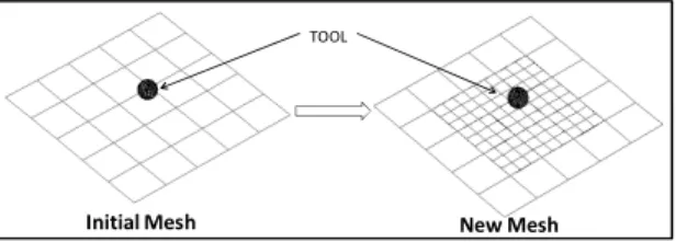
The zone where high deformations occur is always close to the current location of the tool. Therefore, the chosen remeshing method is a refinement without transition which moves along with the tool. The coarse elements, close to the tool, are divided into a fixed number of small new elements. Some new nodes can become inconsistent with the neighbouring coarse elements.
TOOL
Initial Mesh New Mesh
Figure 1 : Remeshing method
2.3 NEIGHBOURHOOD CRITERION
The elements are refined in the tool neighbourhood. The criterion defining the size of the neighbourhood is:
2 2 2
D
≤ α
(L
+
R )
(1)where D is the shortest distance between the centre of the spherical tool and the nodes of the element, L is the longest diagonal of the element, R is the radius of the tool and α is a neighbourhood coefficient chosen by the user. Consequently, every coarse element which respects the criterion is deactivated and refined in several new smaller elements. It becomes a “cell”. In each cell some new objects are generated (nodes, elements, …).
R
L D
Closed Element Refined Element
Figure 2 : Element refinement
2.4 NEW NODES
2.4.1 Generation of new nodes
Each new node is located between two old nodes, A and B. Its degree of freedom is computed by interpolation: p A B
p
p
q
1
q
q
n 1
n 1
= −
+
+
+
(2)where n is the number of new nodes between A and B, p is the new node number, qp, qA and qB are respectively the degrees of freedomof the node p, A and B.
A 1
B 2
p n
: Old Nodes : New Nodes
Figure 3 : Generation of new nodes.
2.4.2 Constrained nodes
This method created some nodes which are incompatible with the non-refined neighbouring element. They must be constrained so that they remain in the same relative positions between two old master-nodes. Consequently there are two types of degrees of freedom q: unconstrained, qf and constrained, qs: f s
q
q
q
=
(3)The constrained degrees of freedom are computed in function of the unconstrained degrees of freedom:
s f
q
=
Nq
(4)where N is an interpolation matrix which contains similar formulae as equation (2). It is then possible to rewrite equation (3) without qs:
f
I
q
Aq with A
N
=
=
(5)where I is an identity matrix.
In order to identify the equilibrium state, the out-of-balance forces matrix F and the stiffness matrix K are modified using the same master-slave relation [6]: T f
F
=
A F
(6) T fK =A K A
(7)where Ff is the out-of-balance forces array and Kf is the stiffness matrix of the unconstrained degrees of freedom.
2.5 NEW ELEMENTS
The new nodes are known but the variables must be transferred from the coarse elements to the new smaller elements. The transfer method used [7] is simpler to implement and requires less computation time than classical ones. The idea is to interpolate a variable (stresses, strains …) from neighbouring integration points using a weighted-average formula. The value of a variable Zj in a new integration point j is computed as equation (8):
p k n n k kJ pj pj min j n n k kJ pj p pj min
CZ
Z
+
R
R
if R >R
1
C
Z
+
R
R
Z if R
R
=
≤
∑
∑
(8)where k are the integration points where the variable Zk is known, p is the closest integration point to the new integration point j where the variable is Zp, Rkj and Rpj are the distance between k and j, p and j respectively, C is an user-defined constant used to amplify the influence of the closest integration point p, n is a interpolation exponent which must be an even number. All the points for which Rkj>Rmax are ignored. After a trial-and-error procedure, the best set of threshold values were found to be: C=5, n=4, Rmax=1.5d where d is a diagonal of the new element and Rmin=10
-5
D where D is a diagonal of the rectangle in which the work piece is inscribed.
2.6 REACTIVATION OF COARSE
ELEMENT
If a cell does not respect the neighbourhood criterion anymore, the new fine elements are removed and the coarse element is reactivated. However the shape prediction could be less accurate if the distortion is important on the location of the coarse element. Consequently, an additional criterion is used.
To assess the distortion, a distance, d, between the current position of every new node, Xc, and a virtual position, Xv, is computed, as illustrated in Figure 4. The virtual position would be the position of the node if it had the same relative position in the plane described by the coarse element. This position is calculated by interpolation with the four nodes positions, Xi, of the coarse element.
v i i
i 1,4
X
H ( , )X
=
=
∑
ξ η
(9)where Hi is the interpolation function, ξ and η are the initial relative position of the node in the cell. The criterion for reactivating a coarse element is:
c v max
d
≤
d
with d = X -X
(10) where dmax is the maximum distance chosen by the user. If the criterion is not respected for a node, then the coarse element is not reactivated and remains a cell with fine elements.d
Old Node New node Virtual position Top view Lateral View
Figure 4 : Example of assessment of distortion in a
cell
2.7 LINKED LIST
In computer science, a linked list [8] is a data structure. It consists of a sequence of objects, each containing arbitrary data fields and one reference (“link") pointing towards the next object. The principal benefit of a linked list over a conventional array is that the order of the linked items may be different from the order in which they are stored in memory or on disk. The list of items can be scanned in a different order. Linked lists facilitate the insertion and removal of objects at any point in the list. During the SPIF process many elements are refined and coarsened, so that many cells are created and removed. This data storage method is appropriate for this purpose. A cell contains the information about new nodes, new element and constrained edges.
CELL CELL
…
CELLPointer Head
pointer
No associated pointer
Figure 5 : Linked list
3
REFERENCE SIMULATION:
LINE TEST
3.1 THE LINE TEST DESCRIPTION
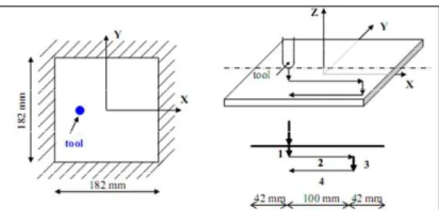
The validation of the new approach is performed on the so-called line test simulation. This simple SPIF test is presented in Figure 6. A square metal sheet of an aluminium alloy AA3003-O with a thickness of 1.2 mm is clamped along its edges. The spherical tool radius is 5 mm. The displacement of the tool is composed of five steps with an initial position tangent to the surface of the sheet: a first indent of 5 mm (step1), a line movement at the same depth along the X-axis (step 2), then a second indent up to the depth of 10 mm (step 3) followed by a line at the same depth along the X-axis (step 4) and the unloading (step5).
3.2 FEM DESCRIPTION
3.2.1 Description of the constitutive law
The elastic range is described by the Hooke’s law. For the plastic part, the yield locus, FHill, is described by Hill’48 law:
( )
(
)
2 2 Hill 11 22 2 2 11 22 12 F1
F
σ
=
H+G σ +(H+F)σ
2
+ 2Hσ σ +2Nσ
-σ =0
(11)where σF is the yield stress and F, G, H and N are Hill’s coefficients. The hardening equation is described by the Swift law:
(
)
nP
F
K
0σ =
ε + ε
(12)where εp is the plastic strain, ε0 is the initial strain before yielding, K is an hardening coefficient and n is an hardening exponent. The parameters of this modelling are summarized in Table 1 to 0.
Table 1 : Hooke’s law parameters
E (MPa) ν 72600 0.36
Table 2 : Hill’48 law parameters
F G H N
1.22 1.19 0.81 4.06
Table 3 : Swift law parameters
ε0 K (MPa) n 0.00057 183 0.229
3.2.2 Boundary Conditions
The geometry and the loading are symmetrical about the X-axis, so that only half of the sheet is modelled. Consequently, the displacements and rotations around the X- and Z-axis are fixed for every node along the X-axis. Moreover, the nodes along the edges are fixed to model the clamping of the sheet.
3.2.3 The meshes
Two types of meshes are tested. The first is the reference. It is used without adaptive remeshing and contains 884 elements. The second is used with adaptive remeshing and contains 314 elements.
Fine mesh for without remeshing simulation
Coarse mesh for with remeshing simulation Figure 7 : Meshes
3.2.4 The remeshing parameters
Every coarse element that needs to be refined is divided into four new elements. The neighbourhood coefficient, α, is equal to 2 and the maximum relative distance, dmax, is 0.1 mm.
3.3 RESULTS
3.3.1 Mesh evolution
Figure 8 shows the evolution of the mesh during the simulation. During step 1, only the elements close to the tool are refined. During the other steps, the tool moves further away. Therefore, some refined elements are removed but those where the distortion is important remain refined. Finally at the end of the simulation the mesh is fine only where the distortion is high.
End of Step 1 Middle of Step 2
End of Step 3 End of Simulation
Figure 8 : Evolution of the mesh
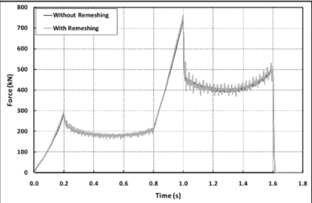
3.3.2 Comparison with the reference
The main outputs of the SPIF simulation are the final shape of the sheet and the evolution of the tool force during the simulation. Figure 9 shows the final shape of the sheet in a cross-section along the symmetric axis in the middle of the thickness for the reference and the remeshed simulation. Figure 10 shows the evolution of the tool force during the simulations. The results are quite similar. The oscillations of the force are due to the penalty method. They are higher with remeshing because the mesh used here is coarser than the reference. -12 -10 -8 -6 -4 -2 0 -100 -80 -60 -40 -20 0 20 40 60 80 100 Z ( m m ) X (mm)
With Remeshing Without Remeshing
Figure 9 : Shape in a cross-section at the end of the
0 100 200 300 400 500 600 700 800 0.0 0.2 0.4 0.6 0.8 1.0 1.2 1.4 1.6 1.8 F o rc e ( k N ) Time (s) Without Remeshing With Remeshing
Figure 10 : Evolution of tool force during the line
test
4
CONCLUSIONS
This paper presents the validation of the adaptive remeshing technique applied on the SPIF process. This method has the advantage to decrease the number of nodes while giving quite accurate results.
In the future the same technique will be used to simulate more complex SPIF process and decrease the time computation.
5
ACKNOWLEGDGEMENT
The authors of this article would like to thank the Institute for the Promotion of Innovation by Science and Technology in Flanders (IWT) and the Belgian Federal Science Policy Office (Contracts IAP P6-24 and TAP2 ALECASPIF P2/00/01) for their financial supports.
As Research director, A.M. Habraken would like to thank the Fund for Scientific Research (FNRS, Belgium) for its support.
6
REFERENCES
[1] Henrard C., Habraken A.M., Szekeres A., Duflou J.R., He S., Van Bael A. and Van Houtte P.: Comparison of FEM
Simulations for the Incremental Forming Process. Advanced Materials Research, 6-8:
533-542, 2005.
[2] Jeswiet J., Micari F., Hirt G., Bramley A., Duflou J. and Allwood J.: Asymmetric Single
Point Incremental Forming of Sheet Metal.
CIRP Annals, 54(2): 623-649, 2005. [3] Cescotto S. and Grober H.: Calibration and
Application of an Elastic-Visco-Plastic Constitutive Equation for Steels in Hot-Rolling conditions. Engineering
Computations, 2: 101-106, 1985.
[4] Jetteur P. and Cescotto S.: A Mixed Finite
Element for the Analysis of Large Inelastic Strains. International Journal for Numerical
Methods in Engineering, 31: 229-239, 1991. [5] Habraken A.M. and Cescotto C.: Contact
between Deformable Solids, the Fully
Coupled Approach. Mathematical and
Computer Modeling, 28(4-8): 153-169, 1998. [6] Driessen B. J., A direct stiffness modification
approach to attaining linear consistency between incompatible finite element meshes.
The Information Bridge, 2000.
[7] Habraken A.M., Contribution to the modelling
of metal forming by finite element model. Ph D
thesis of University of Liege, 1989.
[8] Newell, Allen and Shaw, Programming the
Logic Theory Machine. Proceedings of the
Western Joint Computer Conference: 230-240, 1957.