HAL Id: hal-02749906
https://hal-imt-atlantique.archives-ouvertes.fr/hal-02749906
Submitted on 3 Jun 2020
HAL is a multi-disciplinary open access
archive for the deposit and dissemination of
sci-entific research documents, whether they are
pub-lished or not. The documents may come from
teaching and research institutions in France or
abroad, or from public or private research centers.
L’archive ouverte pluridisciplinaire HAL, est
destinée au dépôt et à la diffusion de documents
scientifiques de niveau recherche, publiés ou non,
émanant des établissements d’enseignement et de
recherche français ou étrangers, des laboratoires
publics ou privés.
Estimation of Electricity Production from Photovoltaic
Panels
Vamsi Bulusu, Yann Busnel, Nicolas Montavont
To cite this version:
Vamsi Bulusu, Yann Busnel, Nicolas Montavont. Estimation of Electricity Production from
Photo-voltaic Panels. CoDIT 2020 : 7th International Conference on Control, Decision and Information
Technologies, Jun 2020, Prague, Czech Republic. pp.1-6, �10.1109/CoDIT49905.2020.9263789�.
�hal-02749906�
Estimation of Electricity Production from
Photovoltaic Panels
Vamsi Bulusu, Yann Busnel and Nicolas Montavont
IMT Atlantique, Irisa, France
Email: {firstname.lastname}@imt-atlantique.fr
Abstract—The electricity grid is evolving to a distributed in-frastructure in which smart grids integrating renewable energies will become dominant. Because of the limited capacity of the battery to store the energy produced at certain time of the day, it is necessary to shift the consumption to when the electricity is actually produced. This paper deals with the estimation of solar panel production in order to forecast when and how much electricity will be available. We propose an Artificial Neural Network model to predict the hourly production of photovoltaic (PV) plants. We evaluate our approach over a large dataset of solar panel electricity production over a period of seven years.
Index Terms—Solar Panel, Renewable Energy, Machine Learn-ing, ForecastLearn-ing, Neural Networks
I. INTRODUCTION
Different efforts are made in the electricity industry toward smart grid [1], a distributed system including microgeneration units using renewable energies. Different use cases drive smart grid deployment: provide electricity to isolated lands (e.g. small islands that are disconnected from the grid) [2], provide electricity with autonomous or inter-connected systems [3], or reduce the dependency on carbon and/or nuclear energy [4]. The major challenges to integrate renewable energies in the grid are instability and intermittent production. Most renewable energy sources are dependant on the weather or other environmental phenomena, such as tides or storms. This adds an intrinsic uncertainty in their production.
A smart grid comes with a communication framework in which components may exchange monitoring and control information [5], [6]. Through a standardized set of protocols, objects talk the same language, and any of them can talk with any other one. The smart meter is certainly the most popular communicating element in the smart grid [7]. It allows to remotely monitor the energy consumption in real time and may also be used to broadcast price information. The bi-directional nature of the communication allows devices to negotiate with each other. Interestingly, it allows consumer devices to exchange information with production units, thus making the system flexible: the consumer devices may adapt their behavior depending on the energy availability, to some extent. For example, the grid may choose the best source and time for dispatching energy when there is a request for supply. In order to fully take advantage of the smart grid, real time monitoring and control is not enough, but predictions are needed [2], [8], [9]. Accurate and reliable forecasting of the
productions can further feed the optimization problem to align the consumption with the production.
Solar energy is one of the largest and fastest-growing sources of renewable energy. Solar power plants range from a few connected solar panels for individual households or small industries to larger PV farm where panels are spread over an area of a 2 - 5 square kilometers. Accurate forecasting of the production can help plan the electricity usage efficiently. Forecasts can also help monitor and maintain solar power plants. While hourly and daily forecasts can help examine the proper functioning of the plant, daily and weekly forecasts can help with scheduling maintenance and long term planning. This paper focuses on forecasting the production for solar microgrids. The microgrids are harder to model using weather data since the weather forecasts are provided for areas accurate up to a couple of square kilometers while the microgrids vary from a few square meters to a couple of hundred square meters in area. For larger PV plants, the inaccuracies in the weather forecasts are compensated by the large area of the power plant. We propose a two-step neural network based model to forecast the hourly production of solar power plants. The first step is the prediction of hourly irradiance values based on the weather forecast. The second step is the hourly production forecast using a separate model to forecast every hour of the day.
The remainder of the paper is as follows. Next section deals with the related work and discuss the most recent works on solar panel production forecast and the main differences with our approach. Section III describes the data set, and gives an overview of our model. Section IV indicates our choices regarding the selected artificial neural network and section V finally presents our model. Section VI presents the results we obtained, and section VII concludes the paper by giving some perspectives.
II. RELATEDWORK
There has been a lot of works in the area of machine learning for solar power production forecasting due to the increase in the urgency to shift to renewable power sources. With the climate change and the price drop of solar panel, smart grids need to better integrate this source of energy into the traditional grid. However, in order to provide a smooth integration, we need to cope with the intermittent production and forecasting the production is key to address this challenge.
Cococcioni et al. [10] propose an interesting model in which the time series nature of the data is exploited. A single neural network is trained to predict the output of the PV plant every 15 minutes. The neural network considered for this approach is a feedforward network with tapped delay lines. The neural network takes as input the irradiance and output values of the previous day corresponding to the same hour. Depending on the number and type of delay lines, the network may consider more observations from the previous day or observations from more days to learn the trend in the irradiance and output values. It then predicts the output production solely based on the time series characteristics of the data. While this approach is suitable for large PV installations in regions with fairly stable weather, smaller installations and locations with erratic weather conditions are not well modelled by this approach.
Dolara et al. [11] show an interesting approach to the problem. The paper proposes a hybrid method to predict hourly power productions in a day-ahead manner. The proposed model consists of a neural network which takes the weather forecast and some temporal features as input. The model also takes the clear sky irradiance values that are calculated based on the deterministic Clear Sky Solar Radiation Algorithm (CSRM) [12]. The neural network is trained to learn the amount of irradiance actually used by the solar plant based on the various weather forecast variables.
Nespoli et al. [13] propose a neural network model that takes the average temperature and average measured irradiance of the previous day to predict the irradiance of the current day. It produces 24 outputs corresponding to the irradiance forecast for 24 hours. The mean of these values is then used to decide between two separate models for sunny and cloudy days based on the mean of the predicted irradiance. The second models then use the mean of irradiance, temperature and production of the previous day to predict 24 values corresponding to the hourly production of that day.
Grimaccia et al. [14] consider a neuro-fuzzy model which feeds into the neural network the weather forecast at 3 different points of the day all at once. The forecasts for 6 A.M., 12.P.M. and 6 P.M. are used together to predict the complete day’s production. The weather forecast supplied to the network also includes a fuzzy logic pre-processed irradiance value for the 3 times of the day.
Lorenzo Gigoni et al. [16] compares several benchmark models such as neural networks, kNN (k Nearest Neighbours) and SVR (Support Vector Machine). The model uses large PV plant data to compare and hence does not show much variation from model to model owing to the averaging of irregularities. This is not the case for micro and nano grids.
In this paper we propose a neural network based model to predict the hourly productions. The model consists of two parts, where the first part uses hourly weather forecast data to predict the irradiance and the second part uses the forecast irradiance values along with the weather and some other processed data to predict the production. The hourly inputs were considered since a lot of the hourly variation in data is lost if the average values are provided as proposed in the
first paper explained. The neural networks in the second part are separate models trained for every hour. This helps the neural network to learn the structural and temporal features separately. Using the same model to predict the value of different hours leads to too much variance in the data for the model to accurately learn important features.
III. DATASET ANDOVERVIEW
A. PV module and Dataset
The used dataset are part of the project Photovolta2 [15]. These data are coming from two separate sets of solar panels, which have the following characteristics:
• Solar panel technology - silicon mono-crystalline
• Panel Inclination - 15
• Panel rating - 960 W
• Total surface area - 5.52m2
• Microgrid Location - Latitude of 471420.76N and
Lon-gitude of 13330 24W
The first dataset contains about 1400 days of observations from 2011 to 2017. The second dataset contains 1000 days from 2014 to 2017. Both contain the measured irradiance values and the output DC power. The weather forecast data contain various variables with an hourly frequency. While the weather forecast provides various variables (such as the UV index, temperature, wind chill, etc.), only some of them will be useful in the forecasting of the hourly production.
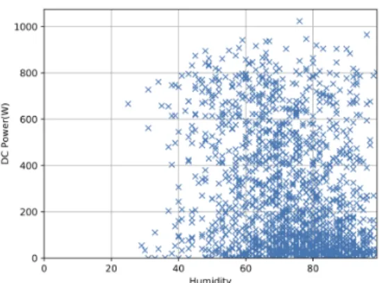
Fig.1 and 2 show the dependency between the DC power and the irradiance, and the humidity respectively. We observe a linear relationship between the irradiance and the DC power, while there is no clear relationship between the humidity and the DC power. However typical weather forecasts do not directly provide irradiance values, thus the need for predicting the irrandiance from other weather variables.
Fig. 3: The proposed two step prediction model
B. Overview
We propose a two step process to forecast hourly production values as shown in Fig. 3. In contrast to Cococcioni et al. [10] who use the previous days record, we use the weather forecast of the target day. This provides a lot more correlation between the inputs and the output. The first step in the proposed method
Fig. 1: Scatter plot between DC power (output) and the irradiance (input)
Fig. 2: Scatter plot between DC power (output) and the humidity (input)
is the prediction of hourly irradiance values from the hourly weather forecast. The second step involves the feeding of the predicted irradiance values along with the weather forecast values and some processed neighbourhood statistics to the hourly models. We propose the use of 15 hourly models to predict the forecast for every hour. These models correspond to the 15 hours between hour 7 and hour 15 of the day. This is especially useful in the case of predictions for microgrids. The hourly models also help in maintaining the inputs unconnected. Providing more than one forecast at a time is recommended for predicting average values but will confuse the network when trying to predict the hourly production. One more reason for the hourly models is that a single model would require 15 output neurons to make hourly predictions but in general, a single neural network with multiple outputs performs better when the outputs are correlated while multiple neural networks with a single output are preferred for uncorrelated outputs.
IV. ARTIFICIALNEURALNETWORKS
Artificial Intelligence methods have become popular in predicting outputs that are complex nonlinear functions of the inputs. Artificial Neural Networks (ANNs) are a popular subclass of machine learning models, which are loosely based on the learning model of a human brain. ANNs are fairly straightforward systems, which process the data with the help of artificial neurons and learn intrinsic features which help map the input to the output. The word intrinsic is used here to stress the fact that the neural network learns without any a priori knowledge about the features.
The ANN method proposed in this paper uses the Multi-Layer Perceptron (MLP) model. An MLP generally consists of an input layer followed by several hidden layers and an output layer. Each layer consists of a predefined number of artificial neurons. Every layer in an MLP starting from the input layer is generally densely connected to the next layer meaning that every neuron in a layer is connected to every other neuron in the next layer. The connections between neurons of consecutive layers carry weights and the neurons then apply an activation function over the weighted inputs and
pass it to the next layer. The usual rule of thumb is that a wider neural network (more neurons per layer) tends to memorize better and a deeper (more hidden layers) neural network is able to learn highly nonlinear features better.
Training algorithms are then used to change the weights of the connections to learn the best mapping between the inputs and the outputs. The best mapping between the input and the output is the solution to the optimization problem of minimizing or maximizing a cost function depending on the type of data. The cost function can be considered to provide some prior knowledge to the model about the kind of mapping. The most famous training algorithm is the error backpropagation based on gradient descent. This algorithm is computationally expensive but converges to a minima fairly easily with the proper learning rate and batch size. The back-propagation algorithm is, however, suitable for the problem described in this paper.
V. DATA ANDNORMALIZATION
A. Data Processing
The data used for the forecasting of the PV power plant productions are (i) the static weather forecast data, (ii) the irradiance prediction and (iii) the DC output from observations with the closest weather conditions. The static weather forecast data is the most important of the three and provides the basis for the predictions. It is mined for the particular location of the solar panels using the latitude and longitude. The weather forecast used for this research was mined using the world weather online API (Application Program Interface) for python. The weather forecast consists of various variables out of which the most suitable subset has been chosen. The weather variables used for the prediction are UV Index, cloud cover, humidity, temperature and visibility.
The irradiance prediction value is obtained from a neural network model that is trained to predict the irradiance values based on the weather forecast variables and past irradiance recordings. This is a way of guiding the neural network to use the features that are known to impact the production of the panels. This intermediate step of predicting known features
that affect the production helps the neural network learn more meaningful patterns. Otherwise, the network tends to learn abstract features which may not be suitable for the problem or may not be present in the testing data.
The nearest weather neighbours are obtained by processing every weather input individually to find the 50 nearest data points from the training set that have the closest weather to the forecast. The distance between two weather observations is calculated using the Euclidean distance between them which is calculated as follows
d(p, q) = d(q, p) =p(q1− p1)2+ · · · + (qn− pn)2 (1)
The power production of these 50 points is then retrieved and sorted. The sorted list of production values is then reduced by removing the highest and lowest 10 points. This is done to effectively remove outliers that may influence the output towards the outlier points. After the reduction of the 50 values into a list of 30 values, the minimum, maximum and the mean values of the list are taken as inputs to the final prediction model.
The irradiance values for any new site can be obtained from satellite data while the PV production values need to be recorded at the site and trained continuously. The model will continually improve as the training period increases and reach a saturation after the first a rolling 8-12 month period is reached.
B. Data normalization
Neural networks tend to perform better when the inputs and outputs of the network are normalized [8]. Normalization generally increases the speed of convergence of the error and does not affect the accuracy. Raw data tends to be in different scales and this leads to different range of weights for different connections making it hard for the gradient descent algorithm to smoothly descend into the minima.
The dataset is divided into a rolling yearly training and testing sets, and each training set is scaled to [0;1] using a Min-Max scaler. The Min-Max Scaler subtracts the minimum values of a feature from every value and divides it by the range (max - min) of the features. The same scaling is then applied to the testing data. The training and testing data are scaled separately to avoid data leakage (some information regarding the future data is used to predict it). This is especially true when using scaling algorithms that involve the mean and variance of the data.
Xscaled=
Xi− Xmin
Xmax− Xmin
(2) C. Model Architecture
In this section, we detail our model architecture, which com-prises two parts. The first part consists of the irradiance model which takes the weather forecast data as input and predicts the irradiance value. This model takes 7 inputs including the 5 weather forecast variables stated above and the corresponding temporal data (day of the year and the hour of the day). It contains two hidden layers with 7 and 4 neurons each with
the ReLU ( Rectified Linear Unit) activation function. The output layer of the model contains a single neuron with a sigmoid activation function since the values are scaled between 0 and 1. This model is trained with the historic irradiance values to forecast future irradiance values as they are not provided as a part of a typical weather forecast. The second part consists of feeding the forecast irradiance values into a second neural network along with the weather forecast data, the nearest neighbours data and the previous day’s production value. Separate models for every hour are not required for the irradiance prediction as we are considering the hourly models to learn the structural and temporal features more accurately, and using them for both the irradiance and power generation predictions will not improve the models accuracy.
Since the predictions are made hourly, we considered sepa-rate models for every hour of the day. The alternative was to consider a network with 24 outputs for every hour of the day but this leads to a decrease in the prediction accuracy due to the increase in the number of features. This increases in the number of features paired with densely connected MLP layers leads to the extraction of unwanted features from forecasts of different hours thereby reducing the accuracy. To obtain a similar accuracy using a single model, we had to use a much wider model which leads to an unnecessary increase in computation. The hourly models are definitely a better option especially for microgrids as they are also able to learn the periodic structural features such as shadows from buildings or obstructions which are significant only during the early and late part of days. The input layer of the hourly models contains 10 features (predicted irradiance, UV Index, cloud cover, humidity, temperature, minimum neighbourhood output, maximum neighbourhood output, mean neighbourhood output, day of the year, previous output for the hour). These hourly models contain two hidden layers with 4 neurons each and an output layer with a single neuron. The first hidden layer uses a ReLU activation function while the second layer has a Tanh (Hyperbolic Tangent) activation function. These activation functions were considered after trying different combinations and evaluating the convergence and accuracy. The output layer has a sigmoid activation function to keep in range with the scaled output values.
VI. RESULTS
The above described model architectures were considered after experimenting with a different number of layers and neurons. The different iterations of the model were evaluated using multiple performance metrics. The performance metric that is most important for such data is the Normalized Mean Absolute Error (NMAE). The NMAE is defined as
N M AE = 1 N N X i=1 |Pmeasured,n− Pf orecast,n| Prated .100 (3)
where Pmeasured is the measured power, Pf orecast is the
predicted power for the same hour and Prated is the rated
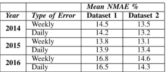
Mean NMAE % Year Type of Error Dataset 1 Dataset 2 2014 Weekly 14.5 13.5
Daily 14.2 13.2 2015 WeeklyDaily 13.813.9 13.113.4 2016 Weekly 16.8 14.6 Daily 16.5 14.3
TABLE I: Yearly NMAE for the 2 datasets
number of observations in a particular day if considering daily NMAE or the number of observations in a week if considering weekly NMAE. The NMAE calculates the error normalized to the size of the system making it suitable to compare systems of different sizes. All other absolute errors cannot be used to directly compare the performance of different systems, owing to the different sizes of solar power plants.
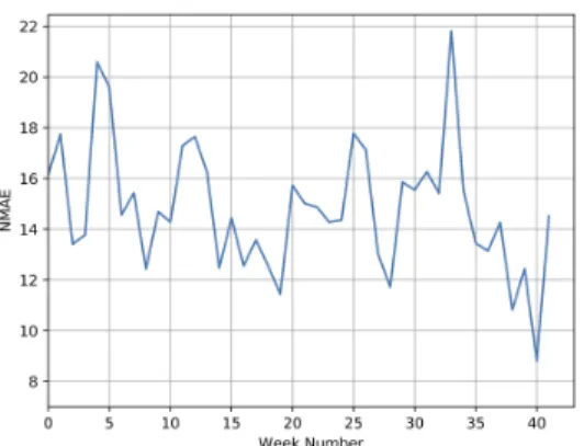
The prediction NMAE for both the data sets can be seen from Table I. It shows the year wise daily NMAE and NMAE averaged over a week. One can observe from Fig. 4 that the weekly NMAE for 42 consecutive weeks from dataset 1 averages at around 15%. The weekly NMAE is calculated by carrying out the sum of the NMAE for all observations in a particular week. Fig. 5 shows the daily NMAE of the same predictions. It can be seen that the NMAE is below 20% for most days. The higher NMAE days have lower overall energy production thereby increasing the relative percentage. The NMAE gives an idea on what percent of error is observed in terms of the total rated power. While simpler models are able to predict with an NMAE below 10% for power plants whose production is in the range of a few 100 KW, they do not work well for smaller installations. Our model allows us to estimate the production with a maximum error of 20%. This accurate predictions are suitable for all the different applications such as unit commitment, electricity market, maintenance scheduling and electricity dispatch planning involving a microgrid.
Fig.7 shows the frequency distribution of the errors for the various hourly predictions cumulated for both data sets. A positive Normalized Error% from this figure corresponds to an underestimated prediction while a negative Normalized Er-ror% corresponds to an overestimated prediction. The fact that the model is underestimating more often than overestimating is of significance advantage as this can give an estimate on the minimum production and can help in planning distributing for the maximum production without overestimating.
Fig. 6 shows the actual and forecast daily energy produc-tions for 100 days from data set 2. The figure also shows the percentage error in green. The percentage error in the plot is the Mean Absolute Percentage Error (MAPE), which is calculated as follows
M AP E = XActual− XP redicted Xactual
.100 (4) It can be seen that the model underestimates most of the time. This is a desirable characteristic in production prediction mod-els as this allows the user to know the minimum production that can be expected. It should also be noted that the MAPE is
considerably high for certain points. MAPE tends to increase with lesser production because it is expressed as a ratio of the production. This however does not mean that the absolute error is high. When considering weekly or monthly productions, the days with lesser productions are insignificant when compared to the total production.
The model was also trained with different time frames of training data for a fixed testing data to evaluate the effect of the training data on the performance of the network. The best results were achieved when the training included the past 12-15 months for forecasting the future 6 months. Any new physical obstructions that might cast shadows on parts of the system or degradation in the infrastructure must be considered while deciding the training period. The solar panels also tend to degrade over the years due to aging and/or improper maintenance. It is therefore recommended not to train on data older than 2 years to avoid inconsistencies between the training and testing data. Fig. 8 illustrates that the model is able to accurately follow the measured power. The results are accurate considering that microgrids are highly sensitive to minute weather and climatic changes.
VII. CONCLUSION
In this paper we focused on the prediction of solar power production. We proposed a novel approach to predict hourly production of PV plants. The proposed model consists of two parts where the first part involved the use of neural networks to extract more appropriate features for the model. The second part involved hourly models which are trained to predict the production for a particular hour using the various input features.
We have evaluated the model for different time frames and applications. It is important to note that the approach is tailored to predict the hourly production of micro and nano grids. The size of the grid is an important factor in the prediction model, in terms of choosing the features and the model architecture. The proposed model is able to predict daily production values with an average NMAE of 15%. This average is over a testing period of 400 days. The weekly NMAE for over 42 weeks averages at 13%.
It can be concluded that using only weather forecast data, the prediction accuracy may reach a limit. This is especially true for microgrids due to the inaccuracies in the weather forecast. Nevertheless, the accuracies of forecast obtained on an hourly, daily and weekly basis are sufficient to benefit the short and medium term planning of solar power plant.
REFERENCES
[1] S. Rahman and M. Pipattanasomporn, Smart grid informa-tion Clearinghouse: Overview of projects and deployment experience, IEEE PES conference on innovative smart grid technologies Latin America (ISGT LA), Medellin, 2011
[2] B. Asato, T. Goya, K. Uchida, A. Yona, T. Senjyu, T. Funabashi, C-H. Kim, Optimal operation of smart grid in isolated island, PEC, Singapore, 2010
Fig. 4: Weekly Normalized Mean Absolute Error Fig. 5: Daily Normalized Mean Absolute Error
Fig. 6: Daily production and forecast Fig. 7: Frequency of occurrence Fig. 8: predicted vs measured for a week [3] N. Anku, J. Abayatcye and S. Oguah, Smart grid: An
assessment of opportunities and challenges in its deploy-ment in the ghana power system, IEEE PES Innovative Smart Grid Technologies Conference (ISGT), Washing-ton, DC, 2013
[4] Xiaoling Jin, Yibin Zhang and Xue Wang, Strategy and coordinated development of strong and smart grid, IEEE PES Innovative Smart Grid Technologies, Tianjin, 2012 [5] G. Habault, M. Lefranois, F. Lemercier, N. Montavont, P.
Chatzimisios and G. Z. Papadopoulos, Monitoring Traffic Optimization in a Smart Grid, IEEE Transactions on Industrial Informatics, vol. 13, no. 6, pp. 3246-3255, Dec. 2017
[6] M. Kuzlu, M. Pipattanasompom and S. Rahman, A com-prehensive review of smart grid related standards and protocols, 5th International Istanbul Smart Grid and Cities Congress and Fair (ICSG), Istanbul, 2017
[7] P. Bansal and A. Singh, Smart metering in smart grid framework: A review, Fourth International Conference on Parallel, Distributed and Grid Computing (PDGC), Waknaghat, 2016
[8] J. Sola and J. Sevilla, ”Importance of input data normal-ization for the application of neural networks to complex industrial problems,” in IEEE Transactions on Nuclear Science, vol. 44, no. 3, pp. 1464-1468, June 1997 [9] M. Marinelli, F. Sossan, G.T. Costanzo, and H.W.
Bind-ner, Testing of a Predictive Control Strategy for Balancing
Renewable Sources in a Microgrid, IEEE Transactions on Sustainable Energy, Vol. 5, No. 4, pp. 1426-1433, 2014 [10] M. Cococcioni, E. D’Andrea and B. Lazzerini,
24-hour-ahead forecasting of energy production in solar PV sys-tems, 11th International Conference on Intelligent Sys-tems Design and Applications, Cordoba, 2011
[11] A. Dolara, S. Leva, M. Mussetta and E. Ogliari, PV hourly day-ahead power forecasting in a micro grid con-text, IEEE 16th International Conference on Environment and Electrical Engineering (EEEIC), Florence, 2016 [12] H. C. Hottel, A simple model for estimating the
transmit-tance of direct solar radiation through clear atmospheres, Solar Energy, vol. 18, pp. 129-134, 1976.
[13] A. Nespoli, E. Ogliari, S. Leva, A. M. Pavan, A. Mellit, V. Lughi, A. Dolara, Day-Ahead PV Forecasting: A Comparison of the Most Effective Techniques. Energies 2019
[14] F. Grimaccia, M. Mussetta and R. Zich, Neuro-fuzzy predictive model for PV energy production based on weather forecast, IEEE International Conference on Fuzzy Systems, Taipei, 2011
[15] N. Barreau, Photovolta2 Project, Universit de Nantes, 2011-2019. URL : http://photovolta2.univ-nantes.fr [16] L. Gigoni et al., Day-Ahead Hourly Forecasting of Power
Generation From Photovoltaic Plants, IEEE Transactions on Sustainable Energy, vol. 9, no. 2, pp. 831-842, 2018