CIRPÉE
Centre interuniversitaire sur le risque, les politiques économiques et l’emploi
Cahier de recherche/Working Paper 05-28
Robust Multidimensional Spatial Poverty Comparisons in Ghana,
Madagascar, and Uganda
Jean-Yves Duclos David Sahn
Stephen D. Younger
Octobre/October 2005
_______________________
Duclos: Département d’économique and CIRPÉE, Université Laval, Canada Sahn: Food and Nutrition Policy Program, Cornell University
Younger: Corresponding author. Food and Nutrition Policy Program, Cornell University [email protected]
This research is supported by the SAGA project, funded by USAID cooperative agreement #HFM-A-00-01-00132-00
with Cornell and Clark-Atlanta Universities, and by the Poverty and Economic Policy (PEP) network of the IDRC. For more information, see http://www.saga.cornell.edu and www.pep-net.org.
Abstract:
We investigate spatial poverty comparisons in three African countries using multidimensional indicators of well-being. The work is analogous to the univariate stochastic dominance literature in that we seek poverty orderings that are robust to the choice of multidimensional poverty lines and indices. In addition, we wish to ensure that our comparisons are robust to aggregation procedures for multiple welfare variables. In contrast to earlier work, our methodology applies equally well to what can be defined as « union », « intersection », or « intermediate » approaches to dealing with multidimensional indicators of well-being. Further, unlike much of the stochastic dominance literature, we compute the sampling distributions of our poverty estimators in order to perform statistical tests of the difference in poverty measures. We apply our methods to two measures of well-being, the log of household expenditures per capita and children’s height-for-age z-scores, using data from the 1988 Ghana Living Standards Survey, the 1993 Enquête Permanente auprès des Ménages in Madagascar, and the 1999 National Household Survey in Uganda. Bivariate poverty comparisons are at odds with univariate comparisons in several interesting ways. Most importantly, we cannot always conclude that poverty is lower in urban areas from one region compared to rural areas in another, even though univariate comparisons based on household expenditures per capita almost always lead to that conclusion.
Keywords: Multidimensional Poverty, Stochastic Dominance, Ghana, Madagascar,
Uganda
1. Introduction
It is common to assert that poverty is a multi-dimensional phenomenon, yet most empirical work on poverty, including spatial poverty, uses a one-dimensional yardstick to judge a person's well-being, usually household expenditures or income per capita or per adult equivalent. When studies use more than one indicator of well-being, poverty comparisons are either made for each indicator independently of the others,3 or are performed using an arbitrarily-defined aggregation of the multiple indicators into a single index.4 In either case, aggregation across multiple welfare indicators, and across the welfare statuses of individuals or households, requires specific aggregation rules that are necessarily arbitrary.5 Multidimensional poverty comparisons also require estimation of multidimensional poverty lines, a procedure that is problematic even in a unidimensional setting.
Taking as a starting point our conviction that multidimensional poverty comparisons are ethically and theoretically attractive, our purpose in this paper is to apply quite general methods for multidimensional poverty comparisons to the particular question of spatial poverty in three African countries, Ghana, Madagascar, and Uganda. We have developed the relevant welfare theory and accompanying statistics elsewhere (Duclos, Sahn, and Younger, 2003). Our purpose in this paper is to give an intuitive explanation of the methods, and to show that they are both tractable and useful when applied to the question of spatial poverty in Africa.
Our poverty comparisons use the dominance approach initially developed by Atkinson (1987) and Foster and Shorrocks (1988a,b,c) in a unidimensional context.6 In a useful review of this literature, Zheng (2000) makes a distinction between poverty comparisons that are robust to the choice of a poverty line and those that are robust to a choice of a poverty measure or index. Both are attractive features of the dominance approach because they enable the analyst to avoid reliance on ethically arbitrary choices of a poverty line and measure. The poverty comparisons that we use here are robust to both the selection of a poverty line and to selection of a poverty measure. In our multidimensional context, this includes robustness over the manner in which multiple indicators interact to generate overall individual well-being.
Section 2 gives a brief description of the data that we use, and an intuitive discussion of multidimensional poverty comparisons. In addition to the stochastic dominance conditions that are familiar from the univariate literature , we discuss two concepts that come up only in a multivariate context. First, we make a distinction between intersection and union definitions of poverty.7 By the well-known focus axiom used in poverty measurement (see for instance Foster, 1984) these definitions identify those over which we wish to aggregate individual poverty statuses to obtain
3 This would involve, say, comparing incomes across regions, and then mortality rates across regions, and so on. 4 The best-known example of this is the Human Development Index of the UNDP (1990), which uses a weighted
average of life expectancy, literacy, and GDP per capita across the population.
5 Such rules have been the focus of some of the recent literature: see for instance Tsui (2002) and Bourguignon and
Chakravarty (2003). Bourguignon and Chakravarty (2002) also give several interesting examples in which poverty orderings vary with the choice of aggregation rules.
6 Atkinson and Bourguignon (1982,1987) first used this approach in the context of multidimensional social welfare. See
also Crawford (1999).
aggregate poverty indices. If we measure well-being in the dimensions of income and height, say, then a person could be considered poor if her income falls below an income poverty line or if her height falls below a height poverty line. This is a union definition of multidimensional poverty. An intersection definition, however, would consider a person to be poor only if she falls below both poverty lines. In contrast to earlier work, the tests that we use are valid for both definitions. In fact, they are valid for any choice of intermediate definitions for which the poverty line in one dimension is a function of well-being measured in the other dimension.
A second key concept that arises only in the context of multivariate poverty comparisons is that, roughly speaking, the correlation between individual measures of well-being matters. We argue that if two populations have the same univariate distributions for two measures of well-being, but one has a higher correlation between these measures, then it should not have lower poverty.8 This is because a person's deprivation in one dimension of well-being should matter more if she is also poorer in the other dimension. The dimensions of well-being are substitutes in the poverty measure. While apparently intuitive, we also present counter-examples, though our poverty comparisons are valid only for the case in which the dimensions are substitutes.
Section 2 closes with examples of why our poverty comparisons are more general than comparisons of indices like the Human Development Index and also comparisons that consider each dimension of well-being independently of the other.
Section 3 applies these methods to spatial poverty comparisons in Ghana, Madagascar, and Uganda. In particular, we compare poverty across region and area (urban/rural) in the dimensions of household expenditures per capita and nutritional status for children under the age of five. Univariate comparisons based on expenditures or nutritional status alone almost always show greater poverty in rural areas in any one region than in urban areas in any other. Bivariate comparisons, however, are less likely to draw this conclusion, for a variety of reasons that we discuss. For this particular application, all of the interesting deviations from the generally accepted conclusion that poverty is higher in rural areas result from the fact that the correlation between these two dimensions of well-being is often higher in urban areas.
Finally, we note that previous work on multidimensional poverty comparisons has ignored sampling variability, yet this is fundamental if the study of multidimensional poverty comparisons is to have any practical application. This paper’s poverty comparisons are all statistical, using consistent, distribution-free estimators of the sampling distributions of the statistics of each poverty comparison.
2. Methods to compare poverty with multiple indicators of
well-being
2.1. Data
The data for this study come from the 1988 Ghana Living Standards Survey, the 1993 Enquête Permanente auprès des Ménages in Madagascar, and the 1999 National Household Survey in Uganda. All of these are nationally representative, multi-purpose household surveys. The first measure of well-being that we use is per capita household expenditures, the standard variable for empirical poverty analysis in developing countries. The second is children’s height-for-age z-score (HAZ), which measures how a child’s height compares to the median of the World Health Organization reference sample of healthy children (WHO 1983). In particular, the z-scores standardize a child’s height by age and gender as follows:
z-score= x xi− median x
σ ,
where xi is a child’s height, xmedian is the median height of children in a healthy and well-nourished
reference population of the same age and gender, and σx is the standard deviation from the mean of
the reference population. Thus, the z-score measures the number of standard deviations that a child’s height is above or below the median for a reference population of healthy children of her/his age and gender.
The nutrition literature includes a wealth of studies showing that in poor countries children’s height is a particularly good summary measure of children’s general health status (Cole and Parkin 1977; Mosley and Chen 1984; WHO 1995). As summarized by Beaton et al (1990), growth failure is “…the best general proxy for constraints to human welfare of the poorest, including dietary inadequacy, infectious diseases and other environmental health risks.” They go on to point out that the usefulness of stature is that it captures the “…multiple dimensions of individual health and development and their socio-economic and environmental determinants (p. 2).” In addition, HAZ is an interesting variable to consider with expenditures per capita because the two are, surprisingly, not highly correlated, so that they capture different dimensions of well-being (Haddad, et.al., 2003).9
2.2. Univariate Poverty Dominance Methods
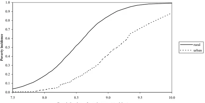
The theoretical and statistical bases for the methods that we use in this paper are developed in Duclos, Sahn, and Younger (2003). In this section, we give an intuitive presentation only – see the appendix for an outline of the formal structure. Even though our goal is to make multidimensional poverty comparisons, it is easier to grasp the intuition with a one-dimensional example. Consider, then, the question addressed in Appleton (2001): did poverty decline in Uganda in the 1990s? The dominance approach to poverty analysis addresses this question by making poverty comparisons that are valid for a wide range of poverty lines and a broad class of poverty measures. Consider Figure 1, which displays the cumulative density functions (cdf) – or distribution functions – for real household expenditures per capita in urban and rural areas of Uganda in 1999. If we think of the values on the x-axis as potential poverty lines – the amount that a household has to spend per capita in order not to be poor – then the corresponding value on the y-axis would be the headcount poverty rate – the share of people whose expenditure is below that particular poverty line. Note that
this particular cumulative density function is sometimes called a “poverty incidence curve.” The graph makes clear that no matter which poverty line one chooses, the headcount poverty index (the share of the sample that is poor) will always be lower for urban areas than for rural. Thus, this sort of poverty comparison is robust to the choice of a poverty line.
Figure 1 - Poverty Incidence Curves, Urban and Rural Areas of Uganda, 1999
0.0 0.1 0.2 0.3 0.4 0.5 0.6 0.7 0.8 0.9 1.0 7.5 8.0 8.5 9.0 9.5 10.0
Cumulative share of sample, poorest to richest
Poverty incidence
rural urban
What is less obvious is that this type of comparison also allows us to draw conclusions about poverty according to a very broad class of poverty measures. In particular, if the poverty incidence curve for one sample is everywhere below the poverty incidence curve for another over a bottom range of poverty lines, then poverty will be lower in the first sample for all those poverty lines and for all additive poverty measures that obey two conditions, that of being non-decreasing and anonymous. By non-decreasing, we mean that if any one person’s income increases, then the poverty measure cannot increase as well. By anonymous, we mean that it does not matter which person occupies which position or rank in the income distribution. It is helpful to denote as Π1 the
class of all poverty measures that have these characteristics. Π1 includes virtually every standard
poverty measure. It should be clear that the latter two characteristics of the class Π1 are entirely
unobjectionable. Additivity is perhaps less benign, but it is a standard feature of the poverty measures because it allows sub-group decomposition. (See Foster, Greer, and Thorbecke, 1984). Comparing cumulative density curves as in Figure 1 thus allows us to make a very general statement about poverty in urban and rural Uganda: for any reasonable poverty line and for the class of poverty measures Π1, poverty is lower in urban than rural areas. This is called “first-order
poverty dominance.” The generality of such conclusions makes poverty dominance methods attractive. However, such generality comes at a cost. If the cumulative density functions cross one
or more times, then we do not have a clear ordering – we cannot say whether poverty is lower in one group or the other.
There are two ways to deal with this problem, both of which are reasonably general. First, it is possible to conclude that poverty in one sample is lower than in another for the same large class of poverty measures, but only for poverty lines up to the first point at which the cdf’s cross (for a recent treatment of this, see Duclos and Makdissi, 1999). If reasonable people agree that this crossing point is at a level of well-being safely beyond any sensible poverty line, then this conclusion may be sufficient. Second, it is possible to make comparisons over a smaller class of poverty measures. For example, if we add the condition that the poverty measure respect the Pigou-Dalton transfer principle,10 then it turns out that we can compare the areas under the crossing poverty incidence curves. If it is the case that the area under one curve is less than the area under another for a bottom range of reasonable poverty lines, then poverty will be lower for the first sample for all additive poverty measures that are non-decreasing, anonymous, and that obey the Pigou-Dalton transfer principle. This is called “second-order poverty dominance,” and we can call the associated class of poverty measures Π2. While not as general as first order dominance, it is still
quite a general conclusion.11
2.3. Bivariate Poverty Dominance Methods
Bivariate poverty dominance comparisons extend the univariate methods discussed above. If we have two measures of well-being rather than one, then Figure 1 becomes a three-dimensional graph, with one measure of well-being on the x-axis, a second on the y-axis, and the bivariate cdf on the z-axis (vertical), as in Figure 2. The bivariate cdf is now a surface rather than a line, and we compare one cdf surface to another, just as in Figure 1. If one such surface is everywhere below another, then poverty in the first sample is lower than poverty in the second for a broad class of poverty measures, just as in the univariate case. It is also useful to note that univariate poverty incidence curves are the marginal cumulative densities in the picture, found at the extreme edges of the bivariate surface.
Figure 2 - Bidimensional Poverty Dominance Surface
10 The Pigou-Dalton transfer principle says that a marginal transfer from a richer person to a poorer person should
decrease (or not increase) the poverty measure. Again, this seems entirely sensible, but note that it does not work for the headcount whenever a richer person located initially just above the poverty line falls below the poverty line due to the transfer to the poorer person.
11 If we cannot establish second order poverty dominance, it is possible integrate once again and check for poverty
dominance for a still smaller class of poverty indices, etc. See Zheng (2000) and Davidson and Duclos (2000) for more detailed discussions.
-3. 82 -3. 32 -2. 82 -2. 32 -1. 82 -1. 32 -0. 82 -0. 32 0.18 0.68 1.18 9.50 10.25 11.00 11.75 0.0 0.1 0.2 0.3 0.4 0.5 0.6 0.7 0.8 0.9 1.0 Cumulative distribution Height-for-age z-score log household expenditure per capita
univariate cdf for household expenditure per capita univariate cdf for HAZ
That class, which we call Π1,1 to indicate that it is first-order in both dimensions of well-being, has
characteristics analogous to those of the univariate case – additive, non-decreasing in each dimension, and anonymous – and one more, that the two dimensions of well-being be substitutes (or more precisely, not be complements) in the poverty measure. This means, roughly, that an increase of well-being in one dimension should have a greater effect on poverty the lower the level of well-being in the other dimension. In most cases, this restriction is sensible: if we are able to improve a child’s health, for example, it seems ethically right that this should reduce overall poverty the most when the child is very poor in the income dimension. But there are some plausible exceptions. For example, suppose that only healthy children can learn in school. Then it might reduce poverty more if we concentrated health improvements on children who are in school (better off in the education dimension), because of the complementarity of health and education.
Practically, it is not easy to plot two surfaces such as the one in Figure 2 on the same graph and see the differences between them, but we can plot the differences directly. If this difference always has the same sign. then we know that one or the other of the samples has lower poverty for a large class Π1,1 of poverty measures. If the surfaces cross, we can compare the distributions at higher orders of
dominance, just as we did in the univariate case. This can be done in one or both dimensions of well-being, and the restrictions on the applicable classes of poverty measures are similar to the univariate case.
Intersection, Union, and “Intermediate” Poverty Definitions
In addition to the extra conditions on the class of poverty indices, multivariate dominance comparisons require us to distinguish between union, intersection, and intermediate poverty measures. We can do this with the help of Figure 3, which shows the domain of dominance surfaces – the (x,y) plane. The function λ1(x,y) defines an "intersection" poverty index: it considers
lies within the dashed rectangle of Figure 3. The function λ2(x,y) (the L-shaped, dotted line) defines
a union poverty index: it considers someone to be in poverty if she is poor in either of the two dimensions, and therefore if she lies below or to the right of the dotted line. Finally, λ3(x,y)
provides an intermediate approach. Someone can be poor even if her y value is greater than the poverty line in the y dimension if her x value is sufficiently low to lie to the left of λ3(x,y).
Figure 3 - Intersection, Union, and Intermediate Dominance Test Domains
For one sample to have less intersection poverty than another for any poverty line up to zy and zx,
its dominance surface must be below the second sample’s everywhere within an area like the one defined by λ1(x,y). To have less union poverty, its surface must be below the second sample’s
and λ3(x,y). The λ(x,y) function delimits the domain over which dominance tests are compared. As
such, it is comparable to the maximal poverty line in a univariate comparison.
Multivariate vs. Human Development Index Poverty Comparisons
Figure 3 is also helpful to understand the difference between the general multivariate poverty comparisons that we use here and comparisons that rely on indices created with multiple indicators of well-being, the best known of which is the Human Development Index (UNDP, 1990). An individual-level index of the x and y measures of well-being in Figure 3 might be written as
I = axx + ayy
where ax and ay are some weights assigned to each variable. This index is now a univariate measure
of well-being, and could be used for poverty comparisons such as those in Figure 1.12 The domain of this test for such an index would follow a ray starting at the origin and extending into the (x,y) plane at an angle that depends on the relative size of the weights ax and ay. Testing for dominance at
these points only is clearly less general than tests over the entire area defined by a λ(x,y)function in Figure 3.
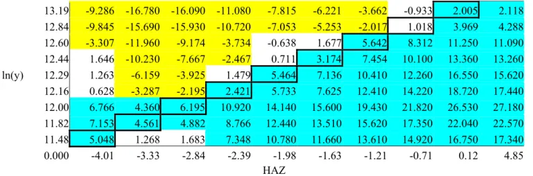
Table 1 gives an example of why our generalization of HDI-type univariate indices is important, comparing poverty in rural Toliara and urban Mahajanga/Antsiranana in Madagascar. The table shows the value of the t-statistic for a test of the difference in the two areas’ poverty surfaces at a 10x10 grid of test points in the domain of Figure 3, i.e. the (x,y) plane of that figure. The origin (the poorest people) is in the lower left-hand corner, and the grid of test points is set at each decile of the marginal distributions.13 We have highlighted the significantly negative differences in light gray (in yellow in the color version) and the significantly positive differences in dark gray (in turquoise in the color version). By choosing the weights ax and ay such that an HDI-type index of these two
dimensions of well-being traces out the diagonal of Table 1,14 we can conclude that poverty is
higher in rural Toliara for a wide range of poverty lines - up to the 70th percentile - and all poverty
measures in the Π1 class. However, another choice of a
x and ay that gives more weight to household
expenditures would yield test points on a steeper ray from the origin and thus imply a significant crossing of the index’s poverty incidence curves, yielding no dominance result. Testing over the entire two-dimensional domain rather than a single ray within that domain avoids this problem.
Table 1 - Π1,1 Dominance Tests for Rural and Urban areas in Toliara, Madagascar
(differences between rural and urban dominance surfaces)
16.51 -8.841 -16.320 -16.580 -11.430 -8.068 -6.658 -4.174 -2.208 0.022 -0.239
12 The Human Development Index is actually cruder than this, as it first aggregates across individuals each dimension
of well-being to generate a single scalar measure, and then constructs a weighted average of those scalars to generate the HDI, which is also a scalar. Dutta, Pattanaik, and Xu (2003) discuss the severe restrictions needed on a social welfare function to justify an index like the HDI.
13 In theory, we should test for differences in the surfaces everywhere, but this is computationally expensive. In
practice, because the surfaces a smoothly increasing functions, it is usually sufficient to test at a grid of points, as we do here.
13.19 -9.286 -16.780 -16.090 -11.080 -7.815 -6.221 -3.662 -0.933 2.005 2.118 12.84 -9.845 -15.690 -15.930 -10.720 -7.053 -5.253 -2.017 1.018 3.969 4.288 12.60 -3.307 -11.960 -9.174 -3.734 -0.638 1.677 5.642 8.312 11.250 11.090 12.44 1.646 -10.230 -7.667 -2.467 0.711 3.174 7.454 10.100 13.360 13.260 ln(y) 12.29 1.263 -6.159 -3.925 1.479 5.464 7.136 10.410 12.260 16.550 15.620 12.16 0.628 -3.287 -2.195 2.421 5.733 7.625 12.410 14.220 18.720 17.440 12.00 6.766 4.360 6.195 10.920 14.140 15.600 19.430 21.820 26.530 27.180 11.82 7.153 4.561 4.882 8.766 12.440 13.510 15.620 17.350 22.040 22.570 11.48 5.048 1.268 1.683 7.348 10.780 11.660 13.610 14.920 16.750 17.340 0.000 -4.01 -3.33 -2.84 -2.39 -1.98 -1.63 -1.21 -0.71 0.12 4.85 HAZ
Multivariate vs. Multiple Univariate Poverty Comparisons
Suppose that one conducts a univariate comparison between expenditures per capita in two samples, as in Figure 1, and children’s heights in two samples, and finds that for both variables, one sample shows lower poverty for all poverty lines and a large class of poverty measures. Is that not sufficient to conclude that poverty differs in the two samples? Unfortunately, no. The complication comes from the “hump” in the middle of the dominance surface shown in Figure 2. How sharply the hump rises depends on the correlation between the two measures of well-being. If they are highly correlated, the surface rises rapidly in the center, and vice-versa. Thus, it is possible for one surface to be lower than another at both extremes (the edges of the surface farthest from the origin) and yet higher in the middle if the correlation between the welfare variables is higher. The far edges of each surface integrate out one variable, and so are the univariate cdf’s depicted in Figure 1. Thus, in this case, one surface would have lower univariate cdf’s, and thus lower poverty, for both measures of well-being independently, but it would not have lower bivariate poverty. Intuitively, samples with higher correlation of deprivation in multiple dimensions have higher poverty than samples with lower correlation because lower well-being in one dimension contributes more to poverty if well-being is also low in the other dimension.15
Table 2 - Π1,1 Dominance Tests for Rural Central vs. Urban Eastern Regions, Uganda
11.660 2.637 12.510 8.720 7.938 9.993 7.941 11.170 4.484 1.109 0.000 9.276 3.458 13.930 9.712 12.030 15.540 15.410 20.020 13.550 14.130 16.400 8.996 5.519 14.940 10.590 13.920 17.110 17.110 22.360 18.330 18.410 20.250 8.803 2.559 11.910 7.156 10.320 13.760 14.730 21.160 18.730 19.030 21.460 8.664 0.610 8.643 4.224 7.651 9.988 9.820 15.270 15.010 16.430 19.950 ln(y) 8.527 0.062 8.763 5.016 8.366 9.201 12.340 17.300 15.860 17.390 19.570 8.395 -2.842 5.754 -0.025 2.692 4.249 6.958 10.650 12.260 13.580 15.240
15 "Correlation" is actually overly strict. For instance, a recent literature has emerged on copulas, namely, functions that
link two univariate distributions in ways that are more general than simple linear correlations but less flexible than our non-parametric distributions. If these copulas differ for two groups, even if their correlations between dimensions of well-being are the same, it is still the case that one-at-a-time univariate dominance results could be reversed with a multivariate comparison.
8.249 -1.582 5.582 -0.307 2.743 2.801 5.305 8.590 11.310 13.020 13.520 8.068 -4.756 1.731 -4.960 -1.046 0.140 2.003 4.765 6.872 9.221 8.636 7.824 4.698 8.001 8.184 9.695 7.846 10.090 12.120 12.850 13.900 12.290 0.000 -3.100 -2.450 -1.970 -1.580 -1.220 -0.880 -0.500 -0.010 0.690 5.820
HAZ
Table 2 provides an example. Univariate poverty is unambiguously higher in rural Central region than urban Eastern region in both dimensions - the difference between the dominance surfaces at the extreme to and right edges is always positive - yet bivariate poverty is not, because of the statistically significant reversal of the dominance surfaces in the interior. Similar comparisons up to third order in each dimension also find that the dominance surfaces cross for these two areas. It is also possible that two samples with different correlations between measures of well-being have univariate comparisons that are inconclusive – they cross at the extreme edges of the dominance surfaces – but have bivariate surfaces that are different for a large part of the interior of the dominance surface. (The sample with lower correlation would have a lower dominance surface). This would establish different intersection multivariate poverty even though either one or both of the univariate comparisons is inconclusive. It could not, however, establish union poverty dominance, since that requires difference in the surfaces at the extremes as well as in the middle.
Table 3 - Π2,2 Dominance Tests for Rural Central and Urban Northern Regions, Uganda
11.660 -0.824 0.263 1.863 1.217 0.048 -1.722 -2.680 -3.454 -3.200 -0.497 9.276 -6.401 -5.347 -4.431 -4.999 -5.578 -6.354 -6.607 -6.573 -5.397 -0.773 8.996 -7.860 -6.909 -6.315 -6.911 -7.340 -7.700 -7.669 -7.393 -6.083 -1.396 8.803 -9.091 -8.169 -7.775 -8.286 -8.554 -8.556 -8.240 -7.784 -6.395 -1.564 8.664 -10.090 -9.240 -8.997 -9.437 -9.571 -9.347 -8.833 -8.222 -6.765 -1.849 ln(y) 8.527 -10.750 -10.000 -9.823 -10.120 -10.080 -9.603 -8.851 -8.014 -6.456 -1.365 8.395 -11.190 -10.360 -10.100 -10.310 -10.300 -9.793 -8.981 -8.069 -6.595 -1.725 8.249 -11.820 -11.280 -10.990 -11.140 -11.190 -10.810 -10.140 -9.274 -7.970 -3.535 8.068 -12.150 -11.680 -11.270 -11.130 -11.010 -10.610 -9.910 -8.959 -7.705 -3.469 7.824 -12.240 -11.870 -11.450 -11.040 -10.650 -10.210 -9.528 -8.628 -7.559 -4.168 0.000 -3.100 -2.450 -1.970 -1.580 -1.220 -0.880 -0.500 -0.010 0.690 5.820 HAZ
Table 3 gives an example. Here, there is no statistically significant univariate dominance in the height-for-age dimension of well-being and only a limited range of poverty lines for which poverty differs in the expenditure dimension, but there is a sizeable domain – up to the ninth decile in each dimension – over which poverty is lower in rural Central region than in urban Northern region for all intersection poverty indices in the Π2,2 class. Thus, for many intersection and intermediate
poverty measures, we can conclude that rural Central region in Uganda is less poor than urban Northern region, despite the fact that neither univariate comparison is conclusive.
In this section, we apply bivariate dominance tests to the question of spatial poverty comparisons in Ghana, Madagascar, and Uganda. We compare poverty in urban and rural areas, nationally and by region,16 measured in terms of household expenditures per capita and children’s height-for-age
z-scores. The tests produce a large amount of output in the form of tables such as Table 1 gives an example of why our generalization of HDI-type univariate indices is important, comparing poverty in rural Toliara and urban Mahajanga/Antsiranana in Madagascar. The table shows the value of the t-statistic for a test of the difference in the two areas’ poverty surfaces at a 10x10 grid of test points in the domain of Figure 3, i.e. the (x,y) plane of that figure. The origin (the poorest people) is in the lower left-hand corner, and the grid of test points is set at each decile of the marginal distributions. We have highlighted the significantly negative differences in light gray (in yellow in the color version) and the significantly positive differences in dark gray (in turquoise in the color version). By choosing the weights ax and ay such that an HDI-type index of these two dimensions of well-being traces out the diagonal of Table 1, we can conclude that poverty is higher in rural Toliara for a wide range of poverty lines - up to the 70th percentile − and all poverty measures in the 1 class. However, another choice of ax and ay that gives more weight to household expenditures would yield test points on a steeper ray from the origin and thus imply a significant crossing of the index’s poverty incidence curves, yielding no dominance result. Testing over the entire two-dimensional domain rather than a single ray within that domain avoids this problem.
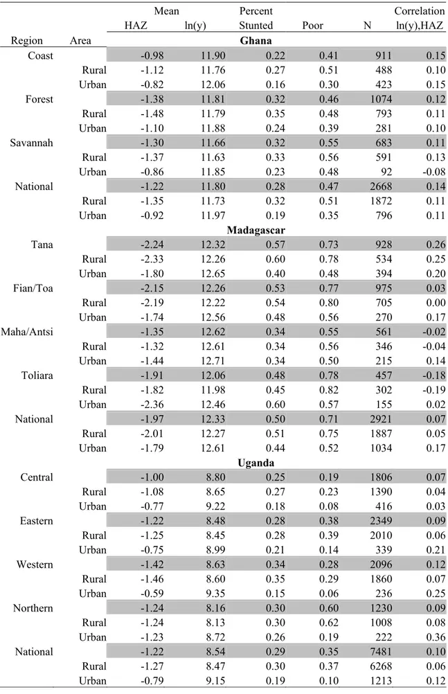
Table 1, which we relegate to appendices.17 Here, we report summaries of the dominance results18. Table 4 gives descriptive statistics for height-for-age z-scores (HAZ) and the log of household expenditures per capita (ln(y)). As one would expect, poverty measured by expenditures per capita and also stunting19 are higher in rural than urban areas in each country. The same is true within
each region of each country, except for Toliara region in Madagascar, where stunting is higher in urban than in rural areas. In fact, with a few exceptions in Madagascar, both expenditure and height poverty are lower in urban areas in any region of each country than in rural areas in any other region in the same country.
In addition to the means and poverty rates, Table 4 also reports the correlation between the log of expenditures per capita and height-for-age z-scores. Note that in Uganda and Madagascar expenditures and heights are more highly correlated in urban than rural areas, while both expenditures and heights tend to be higher in urban areas. As noted above, this combination can cause bivariate poverty comparisons to differ from univariate comparisons carried out separately in each dimension of well-being.20
16 The regions that we use in Ghana are its standard ecological zones of Coast, Forest, and Savannah. In Uganda, we
use the four political regions: Central, Eastern, Western, and Northern. In Madagascar, we also use political regions, but because of small sample sizes, we combined Fianarantsoa and Toamasina, and also Mahajanga/Antsiranana, into single regions. This choice was based on similar agro-ecological characteristics. In all countries, we consider rural and urban areas in these regions.
17 These appendices are available from the authors or at http://www.cfnpp.cornell.edu
18 The relevant statistics and their asymptotic standard errors can readily be computed using the software DAD
(version 4.4 and higher), which is freely available at www.mimap.ecn.ulaval.ca. The authors will also be glad to provide STATA and GAUSS programs that do the same.
19 Stunting usually is defined as a height-for-age z-score of less than –2.
20 It is hard to find universal explanations for the empirical correlations between indicators. The reasons are clearly
context specific. Expenditures and heights may be more highly correlated in urban than in rural areas because in urban areas the use of food markets may be prevalent. Purchasing power would then be better correlated with nutrient intake.
Table 4- Descriptive Statistics for Poverty and Stunting
Mean Percent Correlation
HAZ ln(y) Stunted Poor N ln(y),HAZ
Region Area Ghana
Coast -0.98 11.90 0.22 0.41 911 0.15 Rural -1.12 11.76 0.27 0.51 488 0.10 Urban -0.82 12.06 0.16 0.30 423 0.15 Forest -1.38 11.81 0.32 0.46 1074 0.12 Rural -1.48 11.79 0.35 0.48 793 0.11 Urban -1.10 11.88 0.24 0.39 281 0.10 Savannah -1.30 11.66 0.32 0.55 683 0.11 Rural -1.37 11.63 0.33 0.56 591 0.13 Urban -0.86 11.85 0.23 0.48 92 -0.08 National -1.22 11.80 0.28 0.47 2668 0.14 Rural -1.35 11.73 0.32 0.51 1872 0.11 Urban -0.92 11.97 0.19 0.35 796 0.11 Madagascar Tana -2.24 12.32 0.57 0.73 928 0.26 Rural -2.33 12.26 0.60 0.78 534 0.25 Urban -1.80 12.65 0.40 0.48 394 0.20 Fian/Toa -2.15 12.26 0.53 0.77 975 0.03 Rural -2.19 12.22 0.54 0.80 705 0.00 Urban -1.74 12.56 0.48 0.56 270 0.17 Maha/Antsi -1.35 12.62 0.34 0.55 561 -0.02 Rural -1.32 12.61 0.34 0.56 346 -0.04 Urban -1.44 12.71 0.34 0.50 215 0.14 Toliara -1.91 12.06 0.48 0.78 457 -0.18 Rural -1.82 11.98 0.45 0.82 302 -0.19 Urban -2.36 12.46 0.60 0.57 155 0.02 National -1.97 12.33 0.50 0.71 2921 0.07 Rural -2.01 12.27 0.51 0.75 1887 0.05 Urban -1.79 12.61 0.44 0.52 1034 0.17 Uganda Central -1.00 8.80 0.25 0.19 1806 0.07 Rural -1.08 8.65 0.27 0.23 1390 0.04 Urban -0.77 9.22 0.18 0.08 416 0.03 Eastern -1.22 8.48 0.28 0.38 2349 0.09 Rural -1.25 8.45 0.28 0.39 2010 0.06 Urban -0.75 8.99 0.21 0.14 339 0.21 Western -1.42 8.63 0.34 0.28 2096 0.12 Rural -1.46 8.60 0.35 0.29 1860 0.07 Urban -0.59 9.35 0.15 0.06 236 0.25 Northern -1.24 8.16 0.30 0.60 1230 0.09 Rural -1.24 8.13 0.30 0.62 1008 0.08 Urban -1.23 8.72 0.26 0.19 222 0.36 National -1.22 8.54 0.29 0.35 7481 0.10 Rural -1.27 8.47 0.30 0.37 6268 0.06 Urban -0.79 9.15 0.19 0.10 1213 0.12
We now summarize the dominance results for tests across urban and rural areas in Ghana, Madagascar, and Uganda. For each country as a whole, poverty is higher in rural than urban areas for each univariate poverty comparison and for both intersection and union bivariate comparisons. These results are entirely consistent with virtually every poverty comparison that we know of based on incomes or expenditures alone – poverty is lower in urban areas.
In the regional comparisons, however, a significant number of exceptions to this widely held belief emerge, especially for the bivariate comparisons. Ghana has the fewest of these, with two of nine urban-rural comparisons being statistically insignificant for both intersection and union bivariate poverty comparisons.21 In Uganda, four of sixteen intersection and union comparisons cannot reject
the null of non dominance, and two of these – rural areas in Eastern and Western region vs. urban areas in Northern region – actually have somewhat limited domains over which bivariate poverty is lower in the rural area for intersection poverty measures. In Madagascar, seven of sixteen intersection comparisons and ten of sixteen union comparisons cannot reject the null that bivariate poverty is the same in urban and rural areas, though none of these reject the null in favor of rural areas. While it is true that it is only a minority of cases in which we do not find that urban areas have significantly lower poverty, the fact that there are any such cases is surprising given the overwhelming number of studies that find lower univariate poverty in urban areas in all developing countries.
One immediate concern with these results is that the interesting cases are ones in which we are not rejecting the null of non-dominance, so they may be driven by a lack of power in the statistical tests. This concern is reinforced by the relatively few observations that are available in some urban areas. Review of the appendices shows, however, that in most of the cases in which we do not find bivariate dominance, the dominance surfaces actually cross significantly. That is, there are points in the test domain where the rural surface is significantly above the urban surface and vice-versa. Thus, the lack of bivariate dominance is typically not due to a lack of power.
To gain a better understanding of how bivariate and univariate dominance methods can differ, we classify the results into five types. For type 1, we have dominance (usually first-order) for both univariate comparisons and for intersection and union bivariate comparisons. This is the most common result, accounting for 25 of the 41 comparisons. This is also the least interesting type of result for our methods, because one could ask “why bother with the more complicated bivariate comparisons if, in the end, they produce the same results as simpler univariate dominance tests, or even scalar comparisons?”
Type 2 occurs when neither the univariate nor the bivariate method finds dominance. This is equally uninteresting for our methods. Fortunately, there is only one such case, for urban and rural Mahajanga/Antsiranana region in Madagascar.
Type 3 is a case in which urban areas dominate rural for both univariate comparisons but not for the bivariate comparisons. There are six of these cases. There is also one case, rural Mahajanga/Antsirana vs. urban Toliara, in which the rural area dominates on both univariate
21 In each country, we compare rural areas in each region with urban each regions. Since there are three regions in
comparisons, but not in the bivariate comparisons. For cases in which the bivariate comparisons are inconsistent with the univariate comparisons, a type 3 result is the most common. The bivariate comparisons are more demanding than univariate comparisons, so it makes sense that they reject the null of non-dominance less often, and this happens in five of the seven cases. In two, both involving urban areas in the Northern region of Uganda, the dominance result is actually reversed for intersection poverty measures over a limited domain. This is quite surprising, but understandable once we observe the very high correlation (0.36) between expenditures and heights in urban Northern region compared to rural Western and Eastern regions (0.07 and 0.06, respectively. See Table 4.)
Type 4 occurs when the univariate results are contradictory in the sense that we find univariate dominance in one dimension but not the other. There are six such occurrences, and in all but one we find that the urban area dominates in one dimension, usually expenditures, although there is one case, rural Central vs. urban Northern regions in Uganda, in which the rural area dominates, albeit only for the Π3 class. Of these six cases, we find intersection dominance for four bivariate tests.
That is, the bivariate tests are able to “resolve” the conflicting univariate results for at least some classes of poverty measures22 and areas of poverty lines.
Type 5 is similar to type 4 except that the contradictory univariate results are statistically significant in each univariate comparison. There are only two of these cases, rural vs. urban Toliara, and rural Coast vs. urban Forest in Ghana. Unlike the type 4 results, in neither case are any of the bivariate poverty comparisons statistically significant, so the bivariate comparisons cannot resolve the univariate conflict.
Overall, we certainly have not amassed sufficient evidence to overturn the standard presumption that poverty is lower in urban than in rural areas, but enough of our results are at odds with this idea to give us pause. Further, we have seen that the reasons that we do not find this for bivariate poverty comparisons vary. For the type 4 and 5 cases, we find no univariate dominance in one dimension or another, and the bivariate results follow from that. But this is relatively rare, and in about half of these cases the bivariate tests for intersection poverty measures do actually find that poverty is lower in urban areas despite the contradictory univariate results. Most of the differences, though, come from the fact that our two measures of well-being are often more highly correlated in urban areas than in rural areas. As noted above, this correlation causes the poverty incidence surface to rise more rapidly near the origin of the distribution, raising it above the rural surface in the center even though it is below it at the extremes where we find the univariate poverty incidence curves. In most cases, this gives us results in which an urban area dominates a rural area in each dimension individually, but not jointly, because multiple deprivation is more common in urban areas. There are two cases, however, in which the dominance is actually reversed, so that for some intersection poverty measures, the rural area actually dominates the urban.
4. Conclusions
22 As noted in the methods discussion, bivariate dominance for union poverty measures requires univariate dominance
This paper has used bivariate stochastic dominance techniques to compare poverty in urban vs. rural areas in three African countries, where poverty is measured in terms of expenditures per capita and children’s standardized heights, a good measure of children’s health status. We have shown that our comparisons are more general than either a comparison of a Human Development-type index or “one-at-a-time” comparisons of multiple measures of well-being. More importantly, we find that our more general methods are at odds with simpler univariate poverty comparisons in a non-trivial number of cases.
Expenditure-based urban-rural poverty comparisons almost always find that rural areas are poorer than urban. Our results are consistent with that finding whether we use univariate or bivariate comparisons. However, differences emerge when we compare urban areas in one region of a country with rural areas in another region. We find several cases in which univariate poverty is lower in urban areas in both dimensions, but bivariate poverty is not. This happens because the correlation between expenditures per capita and children’s heights is higher in the urban areas, so that urban residents who are expenditure poor are more likely also to be health poor. This correlation yields a higher density of observations in the poorest part of the bivariate welfare domain for urban areas, even though there are fewer observations for urban residents at the lower end of the density for each individual measure of well-being. We believe that taking such a correlation into account is important for welfare comparisons because the social cost of poverty in one dimension, say health, is higher if the person affected is also poor in the other dimension (expenditures).
It is interesting to note that the share of cases in which urban areas do not dominate rural is much higher in our bivariate comparisons than it is for expenditure- or income-based comparisons in the existing literature, where we almost always find lower poverty in urban areas. We hasten to add, however, that with two exceptions in Madagascar, the urban area in the region where the capital city is located always has lower poverty than every rural area in both univariate and bivariate comparisons. Thus, the doubts that we raise apply only to other urban areas in these countries. There are other instances in which our bivariate comparisons are at odds with univariate comparisons. Perhaps the most interesting are cases in which univariate results are inconclusive because one or the other univariate comparison is inconclusive, yet the bivariate results find dominance for a large domain of intersection poverty indices. This arises in about 10 percent of our examples and occurs again when the correlation between expenditures per capita and children’s heights differs significantly across areas. These results are interesting because they show that bivariate comparisons may actually provide statistically significant results when univariate comparisons do not.
Hence, the finding that bivariate results often differs from the standard perception of greater rural poverty is typically not because children are taller in rural areas, but rather because the correlation between expenditures and heights is lower there than in urban areas. This, however, is based on only three countries: pursuing similar research in other countries will yield insight as to whether these results are anomalous. Why this should be is also an interesting question for future research. But a clear implication of these results for researchers and policy makers interested in multiple dimensions of poverty is that, at a minimum, one should check the correlations between measures
of well-being in the groups of interest. Large differences in these correlations may lead to unexpected multivariate dominance comparisons.
5. Appendix
5.1.
Making poverty comparisons with multiple indicators of
well-being
The following is extracted from our companion paper Duclos, Sahn and Younger (2003).
For expositional simplicity, we focus on the case of two dimensions of individual well-being. Let x and y be two such indicators. Assuming differentiability, denote by
2 ( ) ( ) ( , ): ℜ → ℜ ∂ , ≥ ,0 ∂ , ≥0 ∂ ∂ x y x y x y x y λ λ λ (1)
a summary indicator of individual well-being, analogous to but not necessarily the same as a utility function. Note that the derivative conditions in (1) simply mean that different indicators can each contribute to overall well-being. Assume that an unknown poverty frontier separates the poor from the rich, defined implicitly by a locus of the form λ(x y, ) 0= , and analogous to the usual downward-sloping indifference curves on the (x y space. The set of the poor is then obtained as: , )
{
}
( ) ( ) ( ( ) 0
Λ λ = x y, λ x y, ≤ . (2)
Letting the joint distribution of x and y be denoted by (F x y, ), assume for simplicity that the multidimensional poverty indices are additive across individuals, and define such indices by P( )λ :
( ) ( ) ( ) ( ) Λ =
∫∫
, ; , , P x y dF x y λ λ π λ (3)where π(x y, ;λ) is the contribution to poverty of an individual with well-being indicators x and y : 0 if ( ) 0 ( ) 0 otherwise ≥ , ≤ , ; = . x y x y λ π λ (4)
π is the weight that the poverty measure attaches to someone inside the poverty frontier. By the focus axiom, it has to be zero for those outside the poverty frontier. A bi-dimensional stochastic dominance surface can then be defined as:
0 0 ( ) ( ) ( ) ( ) , , = − − , .
∫ ∫
y x x y z z x y x y x y Pα α z z z xα z y α dF x y (5)This function looks like a two-dimensional generalization of the FGT index and can also be interpreted as such. Our poverty comparisons make use of orders of dominance, s in the x and x s y in the y dimensions, which will correspond respectively to sx =αx +1 and sy =αy +1.
Assume that the general poverty index in (3) is left differentiable with respect to x and y over the set Λ( )λ , up to the relevant orders of dominance, s for derivatives with respect to x and x s for y derivatives with respect to y . Denote by πx the first derivative of π(x y, ;λ) with respect to x , by
y
respect to x and to y . We can then define the following class 1 1,( )∗
Π&& λ of bidimensional poverty indices: ∀ ≥ ∀ ≤ ≤ = = Λ ⊂ Λ = Π y x y x and y x whenever y x xy y x , 0 , 0 0 0 ) , ( 0 ) ; , ( ) ( ) ( ) ( * * 1 , 1 π π π λ λ π λ λ λ && (6)
The first line on the right of (6) defines the largest poverty set to which the poor must belong: the poverty set covered by the P( )λ indices should lie within the maximal set ( )Λ λ∗ . The second line
assumes that the poverty indices are continuous along the poverty frontier. The third line says that indices that are members of 1 1,
Π&& are weakly decreasing in x and in y . The last line assumes that the marginal poverty benefit of an increase in either x or y decreases with the value of the other variable.
Denote by ∆ =F FA −F the difference between a function B F for A and for B . The class of indices defined in (9) then gives rise to the following Theorem:
Theorem 1. 1 1 ( ) 0 ( ) ,( )∗ ∆P λ > , ∀P λ ∈Π&& λ , (7) 0 0 iff ∆P , (x y, ) 0> , ∀ , ∈ Λ(x y) ( )λ∗ . (8) Proof:
Denote the points on the outer poverty frontier λ∗(x y, ) 0= as ( )
x
z y for a point above y and ( )
y
z x for a point above x . The derivative conditions in (1) imply that (1)
( ) 0≤
x
z y and (1)( ) 0≤
y
z x ,
where the superscript (1) indicates the first-order derivative of the function with respect to its argument. Note that the inverse of ( )z y is simply ( )x z x : y x≡z z x . We then proceed by first x( ( ))y integrating equation (3) by parts with respect to x , over an interval of y ranging from 0 to z . y This gives: ( ) 0 0 ( ( ), )= ( , ; ∗) ( ) ( )
∫
y x z z y x y P z y z π x y λ F x y f y dy ( ) 0 0 ( ) ( ) ( ) ∗ −∫ ∫
zy z yx x , ; . x y F x y f y dx dy π λ (9)To integrate by parts with respect to y the second term, define a general function
( ) 0
( )=
∫
g y ( , ) ( , )K y h x y l x y dx and note that:
(1) ( ) ( ) ( ( ) ) ( ( ) ) = , , dK y g y h g y y l g y y dy ( ) 0 ( ) ( ) ∂ , + , ∂
∫
g y h x y l x y dx y ( ) 0 ( ) ( )∂ , + , . ∂∫
g y l x y h x y dx y (10)( ) 0 0 ( ) ( )∂ , − , ∂
∫ ∫
c g y l x y h x y dxdy y (1) 0 ( ) (0) ( ) ( ( ) ) ( ( ) ) = −K c +K +∫
cg y h g y y l g y y dy, , ( ) 0 0 ( ) ( ) ∂ , + , . ∂∫ ∫
c g y h x y l x y dxdy y (11)Now replace in (11) c by z , ( )y g y by ( )z y , (x h x y, ) by πx(x y, ;λ∗), (l x y, ) by (F x y, ) and ( ) K y by its definition ( ) 0 ( )=
∫
g y ( , ) ( , ) K y h x y l x y dx. This gives: ( ) 0 0 0 ( ( ), )= − ( , ; ∗) , ( , )∫
z zx y x x y y y P z y z π x z λ P x z dx (12) (1) 0 0 0 ( ) ( ( ) ) ( ( ) ) ∗ , +∫
zy x , ; , x x x z y π z y y λ P z y y dy (13) ( ) 0 0 0 0 ( ) ( ) ∗ , +∫ ∫
zy z yx xy , ; , . x y P x y dx dy π λ (14)For the sufficiency of condition (8), recall that (1)( ) 0≤
x
z y , 0πx ≤ , and πxy ≥0, with strict
inequalities for either of these inequalities over at least some inner ranges of x and y . Hence, if
0 0, ( ) 0
∆P x y, > , for all y∈ ,[0 z and for all y] x∈ ,[0 z y (that is, for all (x( )] x y, ∈ Λ) ( )λ∗ ), then it
must be that ∆P( ) 0λ∗ > for all of the indices that use the poverty set ( )Λ λ∗ and that obey the first two lines of conditions in (6). But note that for other poverty sets ( )Λ λ ⊂ Λ( )λ∗ , the relevant
sufficient conditions are only a subset of those for ( )Λ λ∗ . The sufficiency part of Theorem 1 thus
follows.
For the necessity part, assume that ∆P0 0, (x y, ) 0≤ for an area defined over ∈[ −, +]
x x x c c and [ − +] ∈ y, y y c c , with + ≤ x y c z and + ≤ ( ) x x
c z y . Then any of the poverty indices in 1 1,( )∗
Π&& λ for which 0
<
xy
π over that area, πxy =0 outside that area, and for which
( , ; ∗)= ( ( ), ; ∗) 0=
x x
y x
x z z y y
π λ π λ , will indicate that ∆ <P 0. Condition (8) is thus also a
necessary condition for the ordering specified in Theorem 1.
Note that similar proofs are possible for dominance comparisons at higher orders. See Duclos, Sahn, and Younger (2003).
5.2.
Estimation and inference
Suppose that we have a random sample of N independently and identically distributed observations drawn from the joint distribution of x and y . We can write these observations of L
x
and y , drawn from a population L , as (L L, L)
i i
x y , i= , ,1… N . A natural estimator of the
bidimensional dominance surfaces x, y( , )
x y
0 0 1 1 ˆ ( ) ˆ ( ) ( ) ( ) 1 ( ) ( ) ( ) ( ) 1 ( ) ( ) , = + + = , = − − , = − − ≤ ≤ = − −
∫ ∫
∑
∑
x y y x y x y x y x x y L z z y x L N L L L L y i x i i y i x i N L L y i x i i z z P z y z x dF x y z y z x I y z I x z N z y z x N α α α α α α α α (15)where ˆF denotes the empirical joint distribution function, ( )I ⋅ is an indicator function equal to 1 when its argument is true and 0 otherwise, and x+ =max(0 ),x . We then have:
Theorem 2. Let the joint population moments of order 2 of ( − A) (+y − A)+x
y x z y α z x α and ( − B) (+y − B)+x y x z y α z x α be finite. Then 1 2/
(
ˆ x, y( , )− x, y( , ))
x y A x y A N Pα α z z Pα α z z and(
)
1 2/ ˆ x, y( , )− x, y( , ) x y B x y BN Pα α z z Pα α z z are asymptotically normal with mean zero, with asymptotic
covariance structure given by (L M, = ,A B ):
(
)
1 ˆ ˆ lim cov ( ) ( ) ( ) ( ) ( ) ( ) ( ) ( ) , , →∞ − + + + + , , , , , = − − − − . − , , x y x y y x y x x y x y x y x y L M N L L M M y x y x x y x y L M N P z z P z z E z y z x z y z x P z z P z z α α α α α α α α α α α α (16) Proof:For each distribution, the existence of the appropriate population moments of order 1 lets us apply the law of large numbers to (15), thus showing that ˆ x, y( , )
x y K z z Pα α is a consistent estimator of ( ) , , x y K x y
Pα α z z . Given also the existence of the population moments of order 2 , the central limit theorem shows that the estimator in (15) is root- N consistent and asymptotically normal with asymptotic covariance matrix given by (16). When the samples are dependent, the covariance between the estimator for A and for B is also provided by (16).
Bibliography
Atkinson, A.B. (2003). "Multidimensional Deprivation: Contrasting Social Welfare and Counting Approaches", The Journal of Economic Inequality 1(1), 51-65.
Atkinson, A.B. (1987). “On the Measurement of Poverty,” Econometrica, 55, 749-764.
Atkinson, A.B. and F. Bourguignon (1982). “The Comparison of Multi-Dimensional Distributions of Economic Status,” chapter 2 in Social Justice and Public Policy, Harvester Wheatsheaf, London.
Atkinson, A.B. and F. Bourguignon (1987). “Income Distribution and Differences in Needs,” in G.R. Feiwel, ed., Arrow and the foundations of the theory of economic policy, New York Press, New York, 350-70.
Appleton, Simon, 2000. “Poverty in Uganda, 1999/2000:Preliminary estimates from the UNHS,” mimeo, Uganda Bureau of Statistics.
Appleton, Simon, 2001, “Poverty reduction during growth: the case of Uganda, 1992-2000,” mimeo.
Beaton, G. H. et al. 1990. Appropriate uses of anthropometric indices in children: a report based on an ACC/SCN workshop. United Nations Administrative Committee on Coordination/Subcommittee on Nutrition (ACC/SCN State-of-the-Art Series, Nutrition Policy Discussion Paper No. 7), New York.
Bourguignon, F., and S. R. Chakravarty (2003). “The measurement of multidimensional poverty,” The Journal of Economic Inequality 1(1), 25-49.
Bourguignon, F. and S.R. Chakravarty, (2002). "Multi-dimensional poverty orderings", DELTA, Paris.
Cole, T. J., Parkin, J. M. 1977. Infection and its effect on growth of young children: A comparison of the Gambia and Uganda. Transactions of the Royal Society of Tropical Medicine and Hygiene 71, 196-198.
Crawford, Ian A. (1999). "Nonparametric Tests of Stochastic Dominance in Bivariate Distributions, with an Application to UK", University College London Discussion Papers in Economics 99/07.
Davidson, R. and J.-Y. Duclos (2000). “Statistical Inference for Stochastic Dominance and the for the Measurement of Poverty and Inequality,” Econometrica, 68, 1435--1465.
Duclos, J.-Y. and P. Makdissi (1999), "Sequential Stochastic Dominance and the Robustness of Poverty Orderings", Cahier de recherche 99-05, CRÉFA, Département d'économique, Université Laval.
Duclos, Jean-Yves, David Sahn, and Stephen D. Younger, (2003), “Robust Multidimensional Poverty Comparisons,” Cornell Food and Nutrition Policy Program, working paper #98. Dutta, I., P.K. Pattanaik, and Y. Xu (2003). "On Measuring Deprivation and the Standard of Living
in a Multidimensional Framework on the Basis of Aggregate Data,'' Economica 70, 197-221.
Foster, J.E., (1984). "On Economic Poverty: A Survey of Aggregate Measures", in R.L. Basmann and G.F. Rhodes, eds., Advances in Econometrics, 3, Connecticut: JAI Press, p. 215-251. Foster, J.E., J. Greer and E. Thorbecke (1984). “A Class of Decomposable Poverty Measures,”
Econometrica, 52 (3), 761--776.
Foster, J.E. and A.F. Shorrocks (1988a). “Poverty Orderings,” Econometrica, 56, 173--177.
Foster, J.E. and A.F. Shorrocks (1988b). “Poverty Orderings and Welfare Dominance,” Social Choice Welfare, 5, 179--198.
Foster, J.E. and A.F. Shorrocks (1988c). “Inequality and Poverty Orderings,” European Economic Review, 32, 654--662.
Haddad, Lawrence, Harold Alderman, Simon Appleton, Lina Song, and Yisehac Yohannes, 2003. "Reducing Child Malnutrition: How Far Does Income Growth Take Us?" World Bank Economic Review 17(1): 107-131.
Mosley,W. H., Chen, L. C. 1984. An analytical framework for the study of child survival in developing countries. Population and Development Review 10(Supplement): 25-45.
Pradhan, Menno, David E. Sahn, and Stephen D. Younger (2003). “Decomposing World Health Inequality,” Journal of Health Economics, 22, 271-293.
Ravallion, Martin, and Benu Bidani, 1994, “How Robust is a Poverty Profile?” World Bank Economic Review 8(1): 75-102.
Shorrocks, A.F., and J. Foster (1987). "Transfer Sensitive Inequality Measures", Review of Economic Studies, 54, 485--497.
Tsui, K, (2002). "Multidimensional poverty indices", Social Choice and Welfare, 19 69--93.
United Nations Development Program (1990). Human Development Report. New York: Oxford University Press.
World Health Organization. 1983. Measuring Change in Nutritional Status: Guidelines for Assessing the Nutritional Impact of Supplementary Feeding Programmes for Vulnerable Groups. WHO, Geneva.
World Health Organization (WHO) 1995. An evaluation of infant growth: the use and interpretation of anthropometry in infants. Bulletin of the World Health Organization 73, 165-174.