ÉCOLE DE TECHNOLOGIE SUPÉRIEURE UNIVERSITÉ DU QUÉBEC
THESIS PRESENTED TO
ÉCOLE DE TECHNOLOGIE SUPÉRIEURE
IN PARTIAL FULFILLEMENT OF THE REQUIREMENTS FOR A MASTER’S DEGREE IN AEROSPACE ENGINEERING
M. Eng.
BY
Alejandro MURRIETA MENDOZA
VERTICAL AND LATERAL FLIGHT OPTIMIZATION ALGORITHM AND MISSED APPROACH COST CALCULATION
MONTREAL, 4 JUNE 2013
© Copyright reserved
It is forbidden to reproduce, save or share the content of this document either in whole or in parts. The reader who wishes to print or save this document on any media must first get the permission of the author.
BOARD OF EXAMINERS (THESIS M. ENG.)
THIS THESIS HAS BEEN EVALUATED BY THE FOLLOWING BOARD OF EXAMINERS
Mme. Ruxandra Mihaela Botez, Thesis Supervisor
Département de génie de la production automatisée at École de technologie supérieure
Mr. Thien-My Dao, President of the jury
Département de génie mécanique at École de technologie supérieure
Mr. Marc Paquet, Member of the jury
Département de génie de la production automatisée at École de technologie supérieure
THIS THESIS WAS PRENSENTED AND DEFENDED
IN THE PRESENCE OF A BOARD OF EXAMINERS AND PUBLIC 30 MAY 2013
ACKNOWLEDGMENT
First, I want to thank Ruxandra Botez for the opportunity she gave me to join this laboratory to finish my project, and the advices and mentorship that she always showed towards me. I would also like to thank Oscar Carranza for his support and advices during this time.
I also want to thank all the members of the laboratory, especially Jocelyn Gagné for his collaboration and suggestions in new implementations, Roberto Felix for his support and, S. Suleymané for his help understanding how to use Flight-Sim and the PTT, Margaux Ruby, Romain Glumineau and Vigninou Akakpo-Guetou for the tests performed.
Finally I would like to thank my family for their understanding and support during my studies.
VERTICAL AND LATERAL FLIGHT OPTIMIZATION ALGORITHM AND MISSED APPROACH COST CALCULATION
Alejandro MURRIETA MENDOZA
RÉSUMÉ
L’optimisation de trajectoires de vol des aéronefs est vue comme une possibilité pour réduire le coût de vol, le carburant consommé, et les émissions des particules qui en découler. L’objective du travail présenté ici est de trouver la trajectoire optimale entre deux points. Pour trouver la trajectoire optimale, les paramètres qui doivent être fournis à l’algorithme sont le poids de décollage de l’avion, les coordonnées initiales et finales de la trajectoire, et l’information météo en la route. L’algorithme donne la trajectoire dans laquelle le coût global de vol est le minimum. Le coût global est un compromis entre le carburant consommé dans une trajectoire et le temps de vol. Il est déterminé avec l’indice de coût, lequel donne un coût en kilogrammes de carburant au temps de vol. L’optimisation dans l’algorithme est réalisée en calculant un profil candidat optimal de trajectoire en croisière. Ce profil est trouvé en réalisant des calculs à l’aide de la « Performance Database » de l’avion. Avec le profil candidat comme référence, différentes croisières sont calculées, et le coût global est déterminé avec l’influence du coût de montée et de descente. Pendant la croisière, des « step climbs » sont évalués pour optimiser le coût de cette phase de vol. Les différentes trajectoires calculées sont comparées et la plus économique est déterminée comme la trajectoire optimale pour le profil vertical.
Avec le profil vertical optimal, différentes trajectoires latérales sont évaluées. En considérant les effets météo, les coûts des routes latérales sont évalués et la route latérale avec le coût global le plus économique est choisie comme la route latérale optimale.
L’information météo a été obtenue du site internet de météo Canada. La nouvelle façon d’obtenir les données du grillage de météo Canada proposée ici aide à économiser les temps de calcul contre des méthodes comme l’interpolation bilinéaire.
L’algorithme développé a été évalué avec deux avions différents : le Lockheed L-1011 et le Sukhoi Russian regional jet. L’algorithme a été développé avec le logiciel MATLAB, et la validation a été effectuée avec l’aide de Flight-Sim de Presagis, et le FMS CMA-9000 de CMC Electronics – Esterline.
À la fin de ce mémoire, la nouvelle méthode pour calculer le carburant consommé pendant les « missed approaches » et ses émissions est développée et expliquée. Les calculs sont faits avec l’aide d’une basse de données et d’un code de Visual Basic développé en Excel.
VERTICAL AND LATERAL FLIGHT OPTIMIZATION ALGORITHM AND MISSED APPROACH COST CALCULATION
Alejandro MURRIETA MENDOZA
ABSTRACT
Flight trajectory optimization is being looked as a way of reducing flight costs, fuel burned and emissions generated by the fuel consumption. The objective of this work is to find the optimal trajectory between two points.
To find the optimal trajectory, the parameters of weight, cost index, initial coordinates, and meteorological conditions along the route are provided to the algorithm. This algorithm finds the trajectory where the global cost is the most economical. The global cost is a compromise between fuel burned and flight time, this is determined using a cost index that assigns a cost in terms of fuel to the flight time. The optimization is achieved by calculating a candidate optimal cruise trajectory profile from all the combinations available in the aircraft performance database. With this cruise candidate profile, more cruises profiles are calculated taken into account the climb and descend costs. During cruise, step climbs are evaluated to optimize the trajectory. The different trajectories are compared and the most economical one is defined as the optimal vertical navigation profile.
From the optimal vertical navigation profile, different lateral routes are tested. Taking advantage of the meteorological influence, the algorithm looks for the lateral navigation trajectory where the global cost is the most economical. That route is then selected as the optimal lateral navigation profile.
The meteorological data was obtained from environment Canada. The new way of obtaining data from the grid from environment Canada proposed in this work resulted in an important computation time reduction compared against other methods such as bilinear interpolation. The algorithm developed here was evaluated in two different aircraft: the Lockheed L-1011 and the Sukhoi Russian regional jet. The algorithm was developed in MATLAB, and the validation was performed using Flight-Sim by Presagis and the FMS CMA-9000 by CMC Electronics – Esterline.
At the end of this work a new method of calculating the missed approach fuel burned and its emissions is developed and explained. This calculation was performed using an emissions database and a Visual Basic for applications code in Excel.
TABLE OF CONTENTS
Page
INTRODUCTION ...1
CHAPTER 1 LITERATURE REVIEW ...5
1.1 Environmental and economical background ...5
1.2 Technological implementations ...8
1.3 Trajectory optimization ...9
1.4 Missed approach ...12
CHAPTER 2 A TYPICAL FLIGHT AND ITS COSTS ...13
2.1 Typical flight ...13
2.1.1 Climb... 14
2.1.1.1 Constant KIAS climb from 2,000 ft to 10,000 ft ... 17
2.1.1.2 Acceleration ... 17
2.1.1.3 Constant KIAS climb and the MACH crossover altitude ... 18
2.1.2 Constant MACH climb ... 18
2.1.2.1 Cruise ... 19
2.1.3 Descent ... 23
2.2 Total flight cost and the cost index ...26
CHAPTER 3 STANDARD ATMOSPHERE, WEATHER AND AIRCRAFT MODEL ...27
3.1 The International Standard Atmosphere ...27
3.2 Altitudes ...29 3.3 Airspeeds ...30 3.4 Earth Model ...32 3.5 Weather model ...33 3.5.1 GRIB2 description ... 34 3.5.2 Data conversion ... 36
3.5.3 Meteorological data interpolation ... 37
3.6 Aircraft model and the Performance database ...40
3.6.1 The performance database ... 40
3.6.2 The performance database interpolation ... 43
CHAPTER 4 FLIGHT TRAJECTORY CALCULATION ...47
4.1 KIAS climb from 2,000 ft to 10,000 ft ...47
4.2 Acceleration ...48
4.3 Constant KIAS climb ...51
4.4 Climb MACH ...53
4.5 Descent distance estimation ...56
4.6 Cruise ...56
4.6.1 Step Climb ... 57
CHAPTER 5 TRAJECTORY OPTIMIZATION ...61
5.1 Vertical navigation optimization ...61
5.1.1 Pre-optimal cruise optimization algorithm ... 62
5.1.2 Pre-optimal cruise results versus the algorithm of reference ... 65
5.1.3 Number of waypoints in the pre-optimal cruise algorithm ... 66
5.1.4 Climb and descent KIAS/MACH selection ... 68
5.1.5 Step climb procedure and selection ... 69
5.1.6 Optimal VNAV route selection ... 71
5.2 Lateral Navigation Optimization ...74
5.2.1 Dijsktra’s Algorithm ... 74
5.2.2 The five routes algorithm ... 77
5.2.3 Coupling VNAV with five routes algorithm ... 78
CHAPTER 6 FUEL CONSUMPTION AND EMISSIONS GENERATED DURING A MISSED APPROACH ...81
6.1 Introduction ...81
6.2 Methodology ...82
6.2.1 Climb/Cruise/Descent CCD mode ... 84
6.2.2 Landing to Takeoff LTO mode ... 87
6.2.3 Crossover calculations ... 90
6.2.4 Full flight cost calculation ... 92
CHAPTER 7 ALGORITHM RESULTS ...93
7.1 Flight calculations validity ...93
7.2 Flight optimization results ...95
7.2.1 L-1011 optimisation tests ... 96
7.2.2 Sukhoi Russian regional jet results. ... 98
7.3 The five routes algorithm results ...100
7.4 Missed approach results ...102
CONCLUSION ...105
LIST OF TABLES
Page
Table 3.1 Vicenty’s methods descriptions ...33
Table 3.2 GRIB2 variables needed in the algorithm ...35
Table 3.3 GRIB2 file nomenclature ...35
Table 3.4 Comparison between closest point to grid ...39
Table 3.5 Sub-databases from the PDB ...40
Table 4.1 Altitudes (ft) of some crossovers for different KIAS/MACH couples ...51
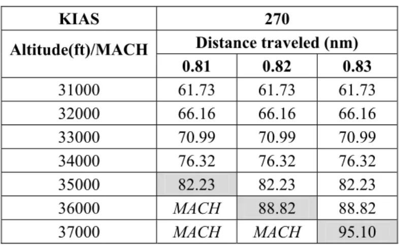
Table 4.2 Distance traveled in a KIAS climb at different crossover altitudes ...52
Table 5.1: Comparison between Gagné’s optimal versus pre-cruise first estimation ...66
Table 5.2 Influence of the cruise computation resolution in the pre-optimal values ...67
Table 5.3 Costs of trajectories at a given altitude...71
Table 5.4 Final cost table ...72
Table 5.5 Comparison between Gil’s shape and the hexagonal shape calculations ...75
Table 5.6 Flight time with static and dynamic weather ...78
Table 6.1 ICAO reference times ...88
Table 6.2 EIG table for the Boeing 737-400 ...89
Table 7.1 Computation fidelity between the algorithm and Flight-Sim ...94
Table 7.2 Flight error between the PTT calculations and Flight Sim...94
Table 7.3 Flight tests for the L-1011 ...96
Table 7.4 Optimisation comparison between the PTT and the algorithm ...97
Table 7.5 Comparison of the profiles provided by the PTT and the algorithm ...97
Table 7.7 Flight cost for a Montreal – Cancun flight with different CI ...98 Table 7.8 Flight cost and time for the five routes algorithm ...101
Table 7.9 Difference in consumption/emissions between full flight with a successful approach and with a missed approach ...102
Table 7.10 Percentage comparison in consumption/emissions between full flight with a successful approach and with a missed approach ...102 Table 7.11 Fuel consumption emissions between a successful approach
and a missed approach ...102 Table 7.12 Consumption/emissions comparison between a successful approach and
LIST OF FIGURES
Page
Figure 1.1 CO2 emissions reduction roadmap ...8
Figure 2.1 Steady flight forces diagram ...14
Figure 2.2 Force diagrams during a typical climb ...15
Figure 2.3 Different stages of climb ...17
Figure 2.4 Weight influence on the fuel flow in a flight at constant speed and altitude ...21
Figure 2.5 Speed influence on the fuel flow at constant ...21
Figure 2.6 Altitude influence on the fuel flow at constant ...22
Figure 2.7 Comparison between different cruises. ...23
Figure 2.8 Force diagram during descent ...24
Figure 2.9 Comparison between the CDA and the stepped descent ...25
Figure 2.10 Flight phases ...26
Figure 3.1 Temperature variation with altitude ...28
Figure 3.2 Wind triangle ...31
Figure 3.3 Global coverage of Environment Canada forecast ...34
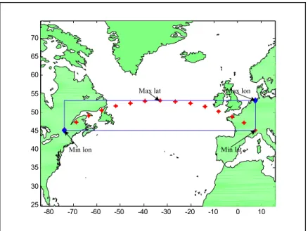
Figure 3.4 Maximum and minimal latitudes and longitudes ...37
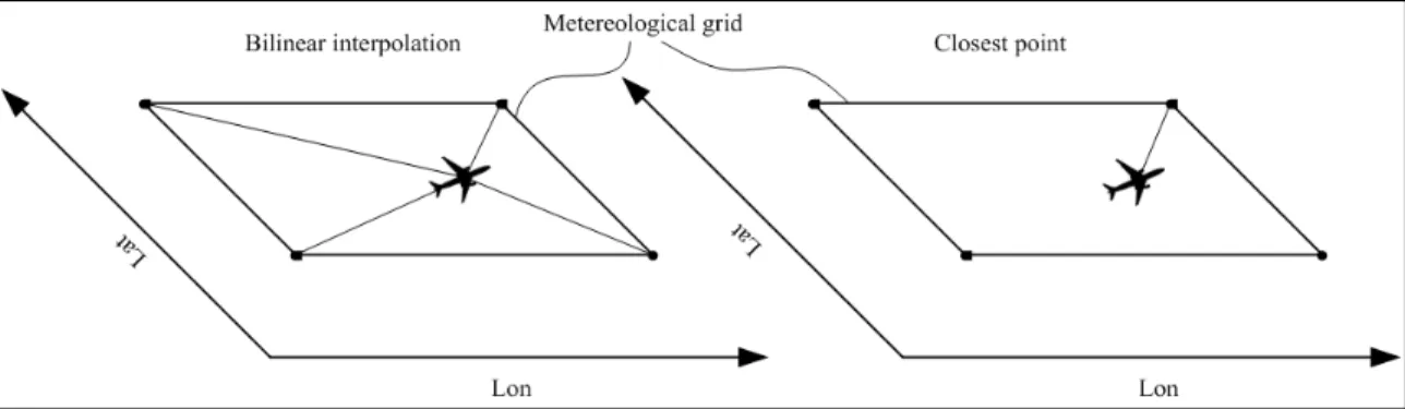
Figure 3.5 Interpolation situation for a given flight ...38
Figure 3.7 Weather interpolation path for a given variable ...39
Figure 3.6 Difference between bilinear interpolations versus the closest grid point ...39
Figure 3.8 PDB output data fetching process ...43
Figure 3.9 Typical PDB data in mode CLIMB KIAS ...44
Figure 3.10 Interpolation path for a desired value ...45
Figure 4.2 Acceleration interpolations path ...49
Figure 4.3 Acceleration during climb and ...50
Figure 4.4 Traveled distance a a climb at 270 KIAS to ...52
Figure 4.5 Horizontal distance traveled to many pairs KIAS/MACH ...54
Figure 4.6 Climb computations flowchart ...55
Figure 4.7 Fuel consumption change with different cruise separations ...57
Figure 4.8 Cruise calculation path ...58
Figure 4.9 Cruise distance separation and descent correction ...59
Figure 4.10 Descent phase calculation procedure ...60
Figure 5.1 Pre-optimal cruise algorithm weights and distances ...64
Figure 5.2 Pre-optimal cruise selection graph ...65
Figure 5.3 Trajectory options for a given altitude cruise analysis ...70
Figure 5.4 VNAV optimization path ...73
Figure 5.5 Gil shape versus hexagon shape ...75
Figure 5.6 Five available lateral routes ...77
Figure 5.7 Five routes algorithm ...79
Figure 6.1 Instrument approach procedure chart ...83
Figure 6.2 A successful approach and landing with a missed approach procedure ...84
Figure 6.3 Polynomial interpolation function versus real data ...86
Figure 6.4 Altitude variation with distance...91
Figure 7.1 Sukhoi RRJ 100 economisation for different trajectories ...99
LIST OF ABREVIATIONS
5RA Five routes algorithm
ATC Air traffic control
ATAG Air transport action group APU Auxiliary power unit CO2 Carbon dioxide
CO Carbon monoxide
CCD Climb/Cruise/Descent
CI Cost index
EIG Emission inventory guidebook EICO Emissions index of carbon monoxide EICH Emissions index of hydrocarbon EINOx Emissions index of nitrogen oxide
EWK Newark
FAA Federal aviation administration
FF Fuel flow
FMS Flight management system
GRIB2 General regularly-distributed information in binary form version 2 GARDN Green aviation research & development network
GS Ground speed
HC Hydrocarbons
ILS Instruments landing system
ICAO International civil aviation organization ISA International standard atmosphere KIAS Knots indicated airspeed
LTO Landing to takeoff
LARCASE Laboratoire de recherche en commande active, avionique et aéroservoélasticité
LNAV Lateral navigation
LHR London Heathrow
LAX Los Angeles
MCL Maximum climbing thrust MNP Minneapolis
NextGen Next generation air traffic management system PTT Part task trainer
PDB Performance database
RoC Rate of climb
RRJ Russian Regional Jet RTA Required time of arrival SESARS Single European sky TOGA Takeoff go around TOC Top of climb TOD Top of descent TAS True ground speed WPT Waypoint
XIX
US United States
UTC Coordinated universal time VNAV Vertical navigation
WA Wind angle
WPG Winnipeg
INTRODUCTION
Lately, there has been a lot of concern in the aerospace industry about fuel needs and the polluting emissions generated by fuel consumption. There is a trend followed by many companies and airlines to deliver products that reduce fuel consumption. Many opportunities in saving fuel, thus polluting emissions, have been identified in the planning aircraft route.
Airlines have ground teams that search and identify the best routes for a given flight. The avionics equipment in the cockpit that helps the pilot to plan and to maintain a route is the flight management system (FMS). The main tasks that a FMS performs according to Collins in [1] are flight guidance, control of the lateral and vertical aircraft paths, monitoring of the flight envelope, computing the optimal speed for every phase of the flight and providing automatic control of the engine thrust, etc. In this work when “optimal” is mentioned, it means the value of the parameters that gives as result the lowest cost of a given flight.
Many different factors such as weather, traffic, or an emergency can change the predefined route given by the ground team. In these events, the crew has to determine a new route using navigation charts or existing FMS algorithms. FMS algorithms compute the “optimal flight altitude” and the “optimal speed”. However, these algorithms need to be improved to find better routes and important data such as weather conditions have to be improved in order to take advantage of favorable winds.
The work in this thesis proposes a new algorithm that finds the optimal vertical navigation (VNAV) route in terms of speed and altitude. A Lateral Navigation (LNAV) route taking advantage of wind patterns is also proposed. A new method to calculate the costs of a missed approach in terms of fuel, flight time and fuel related polluting emissions is introduced. The VNAV and LNAV optimal routes are found by interpolating parameters in the performance databases (PDB) of the aircraft. For the calculations performed in this work, not only the total fuel required to perform a given flight is measured, but also the flight time. The cost calculations are a compromise between fuel burned and time related operations costs.
Required time of arrival (RTA) is not considered as a constraint. For the weather, real data was downloaded from the website of Environment Canada, and then these data were converted into a Matlab file and finally used to calculate the wind effects in flight.
The algorithm proposed does not perform an exhaustive search of all the combinations available in the PDBs to find the “optimal” VNAV profile. The algorithm reduces the possible combinations by defining a “pre-optimal” cruise profile in terms of altitude and speed. The algorithm searches and evaluates different PDB combinations around the “pre-optimal” cruise profile in order to find the ““pre-optimal” profile. Reducing the number of cruise combinations will reduce calculation time comparing with the exhaustive search method.
The trajectories calculated using this algorithm were complete trajectories; this means that climb, cruise, and descent were calculated to decide which trajectory from an initial point at the altitude of 2,000 ft to a final point at an altitude of 2,000 ft was the “optimal”. All data needed for a FMS to guide the airplane is given as the output of the algorithm: KIAS/MACH climb profile, Top of Climb (TOC), cruise speed and altitude, Top of Descent (TOD), MACH/KIAS descend profile and the geographical coordinates that compose the trajectory.
The calculations performed in this algorithm were done for the Lockheed L-1011, from which the laboratory LARCASE has a full aerodynamic model via Flight-Sim, PDB and a FMS Part Task Trainer (PTT), and for the Sukhoi Superjet 100 (RRJ) from which the laboratory also has its PDB and the FMS PTT. All the PDBs were provided by CMC Electronics – Esterline.
The RRJ is a new airplane that started its service in April 2011. These aircraft were designed for medium and long flights. This algorithm focuses on this type of flights, and no optimization is performed for short flights (less than 800 nm). Even if the algorithm was tested and implemented in these two aircraft, it can be implemented in any airplane that has an available PDB.
3
For the new FMSs, optimizations of all routes are searched, that include the missed approach routes. Missed approach (or go around) is a procedure that is implemented when the aircraft has to abort the landing procedure. There are not many documented methods in the literature to compute the missed approach cost.
The work presented in this thesis starts with a literature review to justify and to expose the latest development of this area. Chapter 2 explains the different phases of a typical flight and the costs related to these phases. Chapter 3 describes the models used in this work such as the airplane model or PDB, the atmosphere models, the earth model, etc. In Chapter 4, a description of the calculation performed and considerations made in every flight phase are exposed. Chapter 5 illustrates the optimization method in VNAV used by the algorithm. In Chapter 6 the couple VNAV and LNAV is shown. During Chapter 7, a new method to calculate the missed approach costs is proposed. This calculation may help researchers in the development of algorithms to find the best route when a missed approach procedure is performed. Finally, in Chapter 8, results are presented.
The work presented in this thesis is part of the projects sponsored by the Green Aviation Research & Development Network (GARDN). This project is in collaboration with Esterline - CMC electronics. The name of the project registered from CMC electronics to GARDN is “Optimized Descents and Cruise” in which the objective is to reduce fuel consumptions, thus to reduce emissions.
CHAPTER 1 LITERATURE REVIEW 1.1 Environmental and economical background
Since the first flight performed by the Wright brothers, the aerospace industry has been outstandingly developed. Starting from that unstable aircraft that flew 12 seconds, the aeronautical technology has improved and developed into impressive military aircraft able to cross continents without stopping such as the aircraft B2, or able to fly at speeds higher than sound speed such as the F-22. Research spacecraft have been built, and in some cases, they have even left the atmosphere, such is the case of the space shuttles and the International Space Station.
However, the military industry is not the only one taking advantage of these developments. Civil aviation has also well developed, from small size aircraft used to deliver mail in which many pilots’ lives were lost, to bigger size and safer airplanes such as the A-380 and the 747. These aircraft allow people and cargo to travel between different destinations in a fast and effective way.
Because it is the fastest way to travel, air transportation is one of the preferred ways of traveling; the Air Transport Action Group (ATAG) in [2] estimated that in 2009 only in the United States (US), 704 million passengers were transported by air. This industry can see nothing but growth in the coming years. Boeing estimated that the growth from 2010 to 2030 will be of 5% annually around the globe. Calculations done by the the year 2030 suggested the existence of 5.9 billon passengers around the globe per year. But passengers are not the only ones transported by air; GARDN estimated that in the year 2010 the value of cargo transported by air was of US$5.3 trillion.
In order to meet the needs of such a high volume of passengers and freight, current airports will have to be upgraded and new ones would need to be constructed. Also more aircraft
would be introduced into service; IATA also suggested that by the year 2030 the number of aircraft in service will be of 45,000 around the world.
This high number of aircraft in service will result in a high need of fuel. With a volatile fuel cost, which trend is to be higher each year (In the year 2011, the average value for the Brent crude oil was of US$ 100, US$31 more than in 2010), the new technologies being developed in the aerospace industry target to reduce the fuel consumption in order to reduce the flight cost and improve profit.
In 2008, ATAG in [2] estimated that the most important airlines in the US consumed 19.7 billion gallons of fuel and the American Department of Defence consumed in addition 4.6 billion gallons of fuel to perform their required activities. By the year 2011, the fuel cost needed for the airlines was of 178 billion dollars; this cost is 26% of all the expenses of the airlines.
The needed fuel does not only mean less profit for the airlines, but most importantly: it means pollution. Among the principal emissions from the fuel burned are carbon dioxide (CO2), the combination of nitrogen oxide and nitrogen dioxide (NOx) and hydrocarbons
(HC). The CO2 is one of the major greenhouse effect gases and its release to the atmosphere
is pointed to be one of the principal causes of global warming. In the year 2011, 649 million tons of CO2 where released to the atmosphere by the airplanes. Almost 80% of this CO2 was
released in flights longer than 1000 kilometers where there is no other practical way of traveling. Also 2% of all the CO2 released to the atmosphere is attributable to aviation. HC
also contributes to the greenhouse effect. As mentioned by Ravishankara et al in [3], NOx is
pointed to destroy the ozone layer. This dioxide is released at high altitudes, thus, it is more likely to reach the stratosphere where the ozone layer is located. Another emission that is worth mentioning is vapor water. According with Nojoumi et al in [4], vapor water at high altitudes can cause clouds and can act as a greenhouse gas.
7
The aviation industry is aware of the problem of emissions generated by fuel and proposed itself ambitious goals to reduce emissions in the upcoming years. IATA in [5] reported that since 1960, fuel consumption has been reduced in engines by 80%. However, the aviation industry aims to reduce the fuel consumption and the emissions generated by the aircraft. In 2008 the aerospace industry represented by groups such as IATA agreed to develop what they called the “four pillars” with the aim to reduce fuel consumption and emissions. The first pillar is “the operational process”, such as the reduction of the auxiliary power unit (APU) usage and the weight reduction in flights. The second pillar is “the infrastructure”. Airports are being built and upgraded to meet the new regulations proposed: the Next Generation Air Traffic Management system (NextGen) in the US and the Single European Sky (SESARS). The third pillar which has not yet been implemented consists in the “economic measures”. The fourth and last pillar is “new technology”, such as new materials, new aircraft designs, new engines, new avionic systems, etc.
Using the four pillars mentioned above, what the industry is trying to increase fuel efficiency by 1.5% yearly from 2010 to 2020. The most ambitious goal for the industry is the reduction of CO2 to half its value from 2005 by the year 2050. Figure 1.1 shows the forecast of the CO2
reduction and the influence of every pillar in the goal reduction. This figure also shows the effect of the CO2 emissions if any of the pillars is not implemented.
Figure 1.1 CO2 emissions reduction roadmap
Source: ATAG Beginner’s Guide to Aviation Efficiency (2010, p. 26)
Many associations such as the ATAG, the International Civil Aviation Organization (ICAO) and the Green Aviation Research & Development Network (GARDN) keep track and propose new technologies and methodologies to diminish the emissions.
Emissions and fuel are not the only parameters that these organizations are encouraging to reduce. The interest of noise contamination is also being taken into account. Even though, according to IATA in [5], the noise has been reduced by 75% from 110 dB in 1970 to 90 dB in 2010, it is desirable to reach the 80 dB which is equivalent to car noise at a street intersection or to a lower level.
1.2 Technological implementations
The aeronautical industry has already implemented some new technologies in the last years in order to achieve its ambitious goals. One of the most notable implementations is the winglets. Winglets are the folds at the tips of the wings. This change in the wing geometry helps reducing the magnitudes of the vortices generated by the difference of air between the upper and lower surface of the wing. Reduction of vortices will give induced drag reduction on an airplane. In some cases, winglets also increase the lift coefficient (CL) on a given wing.
9
Boeing in [6] reported an economy of fuel up to 4.4% in a 3,000 nautical miles (nm) flight performed on aircrafts using winglets.
Airlines are also implementing programs to reduce fuel consumption and emissions generated. In the year 2006, as stated in [7], Air Transat added up improvements such as engines washing to improve their efficiency, changing the tires of the fleet to lighter ones, reducing the use of the auxiliary power unit (APU), taxiing with only one engine, reducing the weight of food related items, variation of the cost index (fuel to time ratio) during flight. The fuel consumption was reduced by 5% by Air Transat using the above implementations with some others.
Another technology being developed that would reduce the environmental problems is the biofuel. Different from fossil fuels, biofuels give a reduction of CO2 in every single phase of
their lifecycle. The plants that are ultimately used to generate the biofuel also absorb the CO2
available in the air. Their utilisation, as shown in [8], has shown fewer emissions in comparison with the fossil counterpart. In Canada, as published by the Montreal Gazette in [9], with fundings from the GARDN program, Porter Airlines performed the first biofuel-powered passenger flight in 2012.
Different landing approaches have been developed to reduce fuel consumption such as the Continuous Descent Approach (CDA). The CDA is a type of descent in which the aircraft approaches the runaway in a continuous trajectory, instead to use a traditional step-down descent. IATA in [10] suggested an average reduction of 165 kg of fuel and 523 kg of CO2
for a Boeing 767 in a single descent.
1.3 Trajectory optimization
There is interest in algorithm developments to obtain the optimal trajectory for a given flight. Linden at Honeywell was one of the first researchers that studied the trajectory optimisation for the FMS; his work was concerned mostly the 4D trajectory guidance, (guidance of the
aircraft to arrive at a destination with minimum fuel burn at a given time). In [11], the effects of tailwind, headwind and no wind in the flight cost were studied in the cruise regime by varying the speed, but no step climbs were performed. The optimal cost index was calculated by adding a penalisation if the RTA was not accomplished. This penalisation considered the costs of connection flights lost by the passengers. In [12], a study to determine the effects of the “step climb” in a cruise regime with and without meteorological conditions effects was done. Different methods were developed to determine when it would be the best time to perform a step climb. In [13], the effects of the “step climb” and winds were studied in the search of the optimal cost index for a long flight. A procedure was put in place to get rid of discontinuities in the time versus cost index relationship.
Hougton in [14] recommended parameters to identify such as cloud formation, temperature and usual locations of air currents to locate jet streams during aircraft flight. It discussed the benefits of flying with tailwind and the complexity of an airplane flight at its optimal altitude and the interception gain of a place among other airplanes in a jet stream flight.
Le Merrer in [15] applied the direct method of Herminte-Simpson collocation and the inverse dynamic programming to optimize the flight trajectory and then results obtained by both methods were compared. These methods were developed with the differential equations of an aircraft and optimal control concepts. The solutions obtained with both methods were found to be equivalent.
In our laboratory LARCASE, different optimisation methods for trajectories were found and published by Dancila et al in [16], Felix et al in [17], Gagné in [18] and Fays in [19].
Dancila et al in [16] proposed an algorithm using a PDB to find the best altitude in cruise; measured the time flight and the fuel flow for the A-310, L-1011 and the Sukhoi RRJ 100. In this algorithm, using the cruise trajectories were not divided in sub-trajectories as it is done in the FMS CMA-9000 of CMC Electronics - Esterline. The algorithm gives the same solution as the FMS of reference in 73% of the cases. In this algorithm only the cruise phase was
11
implemented for steady level flights. Climb and descent phases were assumed to have no effect on the flight optimal cruise altitude.
Félix et al in [17] proposed an algorithm using PDB tables found the optimal speed schedule and the optimal cruise altitude using the Golden Section methods for flight distances lower than 500 nm. For flight distances larger than 500 nm, this algorithm evaluated possible step climbs in ever waypoint defined in the route. In this algorithm, a combined mean optimization of 2.57% was attained for the A-310 and L-1011 aircraft with respect to the FMS CMA-9000 algorithm of CMC electronics. Nevertheless, this algorithm needed a complete analysis off all the available pair KIAS/MACH climbs and all the MACH/KIAS descents was needed, that made it time consuming. Besides, this algorithm did not consider the wind effects in the VNAV profile nor an evaluation of the LNAV.
Gagné in [18] proposed an algorithm that found the optimal vertical flight parameters by inspecting the complete trajectory. All possible combinations of climb, cruise and descent were analyzed to find the optimal one. In order to improve the cost reduction during cruise, the possibility of step climbs at each 25 nm was evaluated by measuring fuel flow. A precise method using weather forecast was developed to estimate in an accurate way temperature and wind effects in a flight. Nevertheless, it did not consider lateral navigation (LNAV). Besides, the high number of interpolations needed to perform all flight calculations and weather prediction made the calculation somewhat heavy. It is important to state that this work was a source of inspiration for this thesis.
Another work for the FMS trajectory optimization was developed by Fays. In [19], two algorithms were developed: one to avoid No-Flight-Zones (NFZ) and another one to find the optimal trajectory of an aircraft by combining the methods of descent and tabou. This algorithm was successfully implemented in a Boieng 747-400 and performed a trajectory from Montreal to Paris by avoiding obstacles placed at different altitudes, some in the aircraft trajectory and others outside the aircraft trajectory. The obstacles outside the trajectory were
chosen to prove that the algorithm would not suggest trajectories having obstacles on them.
1.4 Missed approach
In [20], an overview of aircraft trajectory management has been given that would produce noise reduction procedures. Noise produced by flying aircraft was modeled by using fuzzy logic as function of the received noise level during the trajectory, the sensibility of the areas being over flown and the time of the day when the aircraft departure took place. A nonlinear multi-objective optimal control problem was solved in order to find the best trajectory for a given scenario, aircraft and hour of the day. A practical example was given for the departure of an Airbus A340-600 from runway 02 of Girona International Airport. The methodology explained by Prats et al in [20] would assist airspace designers or airport authorities in order to implement noise reduction friendly procedures. The ATR aircraft are recognized in [21] as being the most efficient aircraft in their category, because of their high tech engines and propeller efficiency. The ATR 72-500 gives a 35% fuel saving per passenger with respect to an equivalent turboprop aircraft on a 300 nm average trip. In [21], the influence of flight operations on fuel conservation was examined, with the idea to give recommendations that will enhance the potential for fuel economy.
There have been studies on optimizing runways by maximizing the number of landings per hour in a given runway, in which the number of missed approaches was used as a tool to focus on minimizing costs such as the case of Jeddi in [22]. Nevertheless, a method has not determined in these studies to estimate the cost of missed approaches, instead, a constant value of $4,000 was selected to approximate that cost
CHAPTER 2
A TYPICAL FLIGHT AND ITS COSTS
The theoretical background to understand the ideas implemented in the new algorithm are described in this chapter. In Section 2.1, a typical flight is described so the reader can have a perspective of all the flight phases that have to be calculated in order to find the optimal profile. In Section 2.2, the cost of a flight and the concept of cost index are explained.
2.1 Typical flight
Every day, thousands of aircraft are crossing the sky around the world. All of these flights have different missions. The normal mission for a military aircraft is composed of many flight phases such as take-off, climb, cruise, supersonic dash, target approach at subsonic speed, needed turns around the target, cruise back, descent and landing. Commercial airplanes on the other hand have simpler mission trajectories. Commercial trajectories can be divided in three main flight phases: climb, cruise and descent and normally they do not come back to their departure coordinates as the military aircraft. Those three flight stages have sub-stages that will be explained in detail in the next sections of this chapter.
The quasi-steady flight phases described in flight obey to the equations of motion for an aircraft in translational motion. Because most of the times we are interested in steady unaccelerated flight, after some hypothesis discussed by Anderson [23], these equations can be expressed as
= (2.1)
= (2.2)
Where T is the thrust or power generated by the engines and it can also be seen as power, D is the drag of the aircraft, L is the lift generated by the wings and the airflow speed and finally W is the weight of the airplane. Figure 2.1 shows these forces acting on an airplane.
Figure 2.1 Steady flight forces diagram
Equation (2.1) means that to fly in a steady unaccelerated flight, the force generated by the engines (T) has to equal the drag forces (D) caused by the wind, the plane surfaces and the induced drag of the wings. If thrust happens to be less than the drag, a reduction of speed will be experimented; while if thrust is higher than drag, an augmentation of speed will be experimented by the aircraft.
Equation (2.2) implies that the force that pushes the airplane up (L) has to be equal to the weight (W) of the aircraft. If the lift is higher than the weight, then the airplane would begin to gain altitude. Otherwise, the aircraft would begin to lose altitude.
Equations (2.1) and (2.2) are highly coupled, thus a change in one of them will strongly affect the other one. A complete discussion of these equations can be found in the literature such as [23] and is not discussed in this work.
2.1.1 Climb
In a real flight, taxi and take-off are the first phases, but in this algorithm these phases are not considered because of the lack of experimental data and the regulations that change in many
15
airports around the world makes it difficult to create a generic algorithm. After take-off, the climb is the next phase, and it is calculated by the algorithm beginning at the altitude of 2,000 ft. There are many different engine climb configurations; the one used for the algorithm, is the Maximum Climbing Thrust (MCL). This configuration was chosen because it is the one that needs less fuel to climb than others. In this phase, the thrust generated by the engines is higher than the drag of the airplane because more power is needed in order to climb than it is needed to perform cruise. Also, this is the phase that requires the most fuel of all in a ratio of kg of fuel per nautical mile traveled. The reason is that the aircraft begins its flight at low altitude where the engines are less efficient, therefore more thrust is needed to find the solution of equation (2.1). Figure 2.2 is the force diagram for a typical climb.
Figure 2.2 Force diagrams during a typical climb
By inspecting Figure 2.2, it can be seen that thrust does not only have to compensate the effects of drag, but also some of the forces generated by the weight. This means that more fuel will be needed to produce the needed thrust.
Equations (2.1) and (2.2) have to be changed to include the angle of climb (γ) effect; these equations take the next form:
= + sin γ (2.3)
= cos γ (2.4)
Equations (2.3) and (2.4) express the influence of the weight due to the angle of climb of a given aircraft. The most interesting case is equation (2.3) because it is directly related to fuel consumption. If the angle of climb were to be 90 degrees, the weight and the drag forces would all be carried on and actually equal by the force generated by the engines (thrust) to gain more altitude. In a commercial flight however, this extreme situation will never happen. Still, the climb angle can reach levels of 20 degrees making this effect notorious by the fuel consumption.
In this phase the Rate of Climb (RoC) becomes evident. RoC is the vertical velocity of an aircraft and can be defined as:
≡ ∙ sin γ (2.5)
Equation (2.5) implies that the faster the aircraft flies at a given angle of climb, the faster it will reach the desired altitude, or TOC, the climb phase duration can be reduced to a minimum while increasing the aircraft speed. Nevertheless, climbing too fast may result in an expensive climb.
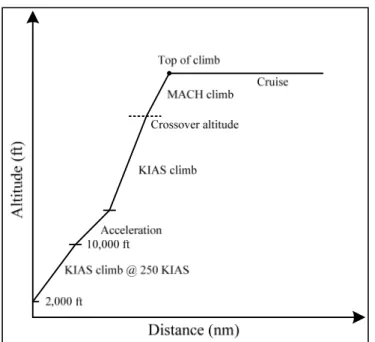
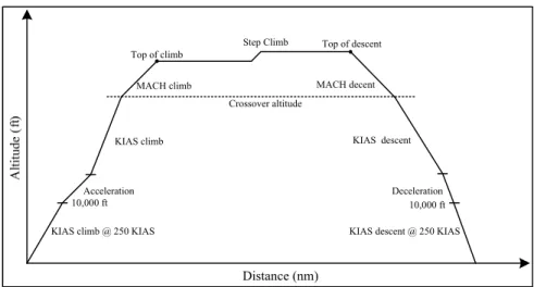
The climb phase is identified by its scheduled speeds, for example 280/0.78. The 280/0.78 means a constant climb at 280 Knots Indicated Air Speed (KIAS) and followed by a constant climb at 0.78 MACH (this speed change takes place after the crossover altitude) until the TOC is reached. Sometimes, in the beginning of a climb, the KIAS is lower than the one needed. In those cases acceleration will be performed to arrive at the desired KIAS before reaching the MACH climb. Figure 2.3 shows the typical phases of a climb that will be described in the next sub-sections.
17
Figure 2.3 Different stages of climb
2.1.1.1 Constant KIAS climb from 2,000 ft to 10,000 ft
The climb phase begins after the take-off, and it is done at a constant KIAS. For the algorithm developed, this part begins at a given geographical point at 2,000 ft. At this altitude, according to [32] until the altitude of 10,000 ft, the aircraft cannot fly faster than 250 KIAS. For this reason the algorithm presented here will never exceed that speed, the aircraft speed will remain within those altitudes in this first stage.
2.1.1.2 Acceleration
When the airplane reaches 10,000 ft, the needed KIAS may be higher than the limit of 250 KIAS. Being that the case, more thrust will be needed to increase the KIAS of the aircraft to the KIAS needed.
2.1.1.3 Constant KIAS climb and the MACH crossover altitude
Once the targeted speed is attained after the acceleration, a constant climb is performed by the aircraft until the TOC is reached or until the MACH crossover altitude is reached, whichever happens first. When the MACH crossover altitude is reached, the crew may have to change the autopilot speed reference from KIAS to MACH. The MACH crossover altitude can be defined as the altitude where the true air speed (TAS) of KIAS equals the scheduled MACH number (in TAS) and depends on the scheduled KIAS/MACH profile climb. Mathematically, the TAS for a given MACH at a given altitude is expressed in knots as shown in equation (2.6) where c is the desired speed of sound in MACH and TASC is the
speed of sound at a given altitude.
= ∙ (altitude) (2.6)
It is really important to change the autopilot reference speed from KIAS to MACH, otherwise, once the MACH crossover altitude is surpassed, and more altitude is gained during the climb phase, the aircraft will fly faster than the expected KIAS, and the MACH would be closer to the speed of sound. Commercial aircraft are not normally designed to fly at such high speeds and fatal consequences may arrive if those speeds are reached.
2.1.2 Constant MACH climb
After the MACH crossover altitude, the climb continues at a constant MACH until the TOC or to the maximum altitude that the aircraft can reach. The speed of sound decreases with altitude that also varies with temperature. The speed of sound is proportional to the temperature which gradually descends with the altitude until the troposphere where it remains constant. The function that defines the speed of sound in a perfect gas is described in equation (2.8).
19
= ∙ ∙ (2.8)
where γ is the adiabatic coefficient index of the air with an adimensional value of 1.4. R is the gas air constant with a typical value of 287 J/kg K, and T is the temperature of the air in Kelvin at a given altitude. It can be noticed that the speed of sound depends only on the temperature. The MACH number is calculated by dividing the actual TAS to the sound speed at a given altitude as expressed in equation (2.9).
= (2.9)
2.1.2.1 Cruise
The cruise is the most important phase of flight; it begins at the TOC and ends at the TOD. It is typically the longest part of the flight, where the most fuel is spent, and more opportunities of optimization exist. For every MACH, the aircraft has to provide the needed lift. During flight, the weight of the aircraft diminishes due to the fuel burned and affects equations (2.1) - (2.2), in order to keep their solution satisfied at a constant altitude-speed, the angle of attack of the aircraft has to be changed during flight. However, changing the angle of attack is a problem that it is not dealt here because the data available in the PDB considers this angle change.
There are three important things that strongly affect the fuel consumption during cruise: weight, speed and altitude. Equation (2.10), (2.11) and (2.12) show the relationship of the thrust with weight, lift and drag.
= / = / (2.10) = 1 2∙ ∙ ∙ ∙ (2.11)
= 1
2∙ ∙ ∙ ∙
(2.12)
CL is the aerodynamic lift coefficient which depends on the angle of attack. CD is the
aerodynamic coefficient of drag which is the sum of a fixed value due to the aerodynamics of the aircraft and the influence of the CL (induced drag), ρ is the density of air, V is the speed of
the aircraft and S is the area of the surface of the wing. Equation (2.10) directly relates weight with thrust. The ratio of lift and drag will normally be higher than one. Then it can be seen that the more the aircraft weighs, the more thrust will be needed, and thus more fuel. It is important to mention that when L/D is at its maximum the thrust would be at its minimum. Equation (2.12) shows that drag is directly proportional to the square of the speed, which means that the faster the aircraft flies, the more drag will be produced. Recalling equation 2.1 this affects directly the thrust needed, thus more fuel.
The last of the main factors that affect the airplane fuel consumption is the altitude. In equation (2.12), the density of the air is identified. The density of air diminishes at high altitudes, causing the drag to be lower at high altitudes, thus reducing the thrust needed. Figures (2.4) – (2.5) show the ideas explained above.
21
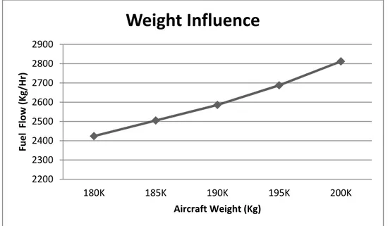
Figure 2.4 Weight influence on the fuel flow in a flight at constant speed and altitude
Figure 2.5 Speed influence on the fuel flow at constant altitude and weight
2200 2300 2400 2500 2600 2700 2800 2900 180K 185K 190K 195K 200K Fuel Flow (Kg/Hr) Aircraft Weight (Kg)
Weight Influence
2200 2250 2300 2350 2400 2450 2500 2550 2600 2650 0,78 0,79 0,8 0,81 0,82 0,83 0,84 Fuel Flow (Kg/Hr) Mach numberSpeed influence
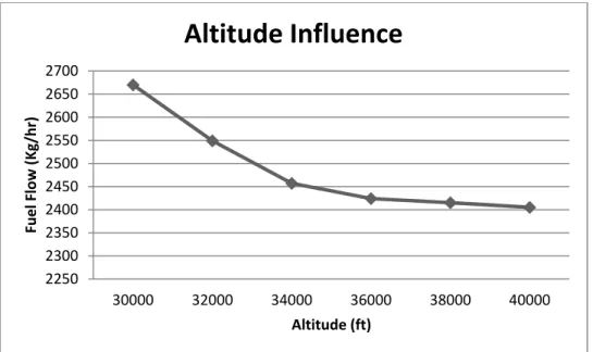
Figure 2.6 Altitude influence on the fuel flow at constant speed and weight
Figures (2.4) - (2.6) were traced with data obtained directly from the PDB of the L-1011. Figure (2.4) shows the influence of the weight on the fuel flow for a flight at 36,000 ft and 0.82 MACH. As expected, the fuel flow tends to be higher as weight is increased. Figure 2.5 shows the influence of the speed in a flight at 36,000 ft with a weight of 180,000 kg. As explained before, the faster the aircraft flies (MACH increases), the more fuel it needs to satisfy the equilibrium conditions at the desired speeds. Finally, Figure 2.6 shows the effect of the altitude on the fuel flow for a weight of 180,000 kg at 0.82 MACH. The higher the aircraft flies, the lower the fuel flow is.
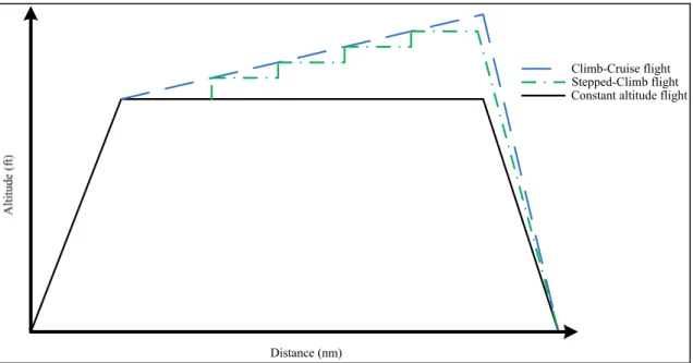
As studied by Ojha [24], the ideal cruise is the one called climb-cruise. This cruise is not performed at constant altitude, but it climbs gradually as the weight of the aircraft is reduced. However, this kind of cruise cannot be implemented because it does not meet the current air traffic control (ATC) regulation, which requires the airplane to flight at a constant altitude and speed. Nonetheless, ATC may allow a climb to a different altitude after traveling a certain distance. This gives an opportunity to emulate the cruise-climb flight by changing altitudes during cruise. While flying at a given altitude, the aircraft asks authorization to the ATC to perform a climb to the next available altitude, and continues its trajectory at that new
2250 2300 2350 2400 2450 2500 2550 2600 2650 2700 30000 32000 34000 36000 38000 40000 Fuel Flow (Kg/hr) Altitude (ft)
Altitude Influence
23
altitude. This flight is called stepped-altitude flight and the climbs performed are called “step climbs”. These step climbs are normally performed for 2,000 ft or 4,000 ft climbs depending on the region, length of flight and the airline preferences. These climb steps are pairs in order to maintain the cruise in an even or pair altitude. In high traffic area even altitudes are assigned to traffic going to one direction and pair altitudes to the aircraft going to the other. Figure 2.7 is a graphical description of the constant altitude flight, climb-cruise flight and the stepped-altitude flight.
Figure 2.7 Comparison between different cruises.
2.1.3 Descent
This is the last phase of flight. It is also identified in a flight speed schedule as the climb phase, for example as MACH/KIAS/KIAS. Beginning the descent in MACH, the aircraft arrives at crossover altitude similar to that in the climb phase. After the crossover altitude, the crew has to change the speed to KIAS and then decelerate to a speed of at least 250KIAS at an altitude of 10,000 ft. It is the phase of flight in which the least fuel is spent. This is due to the fact that the lift of the aircraft diminishes allowing the aircraft to lose altitude. Because lift diminishes, the induced drag caused by the lift is reduced, and then the drag that has to be
Constant altitude flight Climb-Cruise flight Stepped-Climb flight
generated by the engines is further reduced. Also the flight path angle (γ) makes the nose of the aircraft to descend below the horizontal as shown in Figure 2.8. This allows the weight to produce some a part of the forces to maintain the equilibrium in the system that in the other stages of flight would be produced entirely by the thrust. Figure 2.8 describes the force diagram for a descent flight where the thrust is present.
Figure 2.8 Force diagram during descent
= − ∙ sin (2.15)
= ∙ cos (2.16)
Equation (2.15) shows the relationship of the weight with the thrust. In the case of engines failure, the aircraft can maintain the needed thrust (and reduce the lift losing rate) by selecting the proper γ angle. In equation (2.16), lift must be lower than weight because the airplane is descending, having an equal value would mean that the aircraft is maintaining the same lift as weight thus at constant altitude.
Basically, there are two different procedures for descent: the stepped-descent and the Continuous Descent Approach (CDA). During the first approach, the aircraft begins its descent to a given altitude and performs a small cruise, descending then to the next altitude, to maintain a short cruise and so on until the Instrument Landing System (ILS) altitude is
25
reached. This procedure is fuel consuming because it requires cycling the engines from idle to required thrust many times. In the second approach, the airplane descending angle is set approximately to 3 degrees, idles the engines and gliding descent to intercept the ILS altitude to finally reach the runway. The algorithm described in this thesis utilizes this last one to perform landing calculations. The CDA has been successfully implemented and tested in many airports such as Los Angeles (LAX), London Heathrow (LHR) and Newark (EWR). Figure 2.9 shows a graphic difference between these two landing approaches.
Figure 2.9 Comparison between the CDA and the stepped descent
Figure 2.10 Flight phases
2.2 Total flight cost and the cost index
Flights cannot only be measured by how much fuel they need to fly on a given distance. There are many factors that influence the cost such as the salary of the crew, the maintenance cost of an aircraft, the cost of arriving too late or too early to a given gate, among others. A way to calculate the cost used often by airlines and by the FMS is the Cost Index (CI).
The CI allows a compromise between the cost of fuel and time related costs. A higher CI would give priority to a short flight time because the cost of time goes up, while a low CI would give priority to fuel consumption because the flight time is considered to be less important. The expression that defines the total flight cost is defined in eq (2.17) where the total cost, and the total fuel consumed is expressed in kg, the flight time (T) is expressed in hours and the CI in kg/hr, 60 is a conversion to minutes to be able to compare results.
( ) = + ( /ℎ ) ∙ (ℎ ) ∙ 60 (2.17)
While it is possible to change the CI in flight, in the work presented here it is always kept constant. In this work, when the word “cost” is used, it refers to the cost including the CI influence. The CI value is always selected by the airline and can change from one flight to another.
Distance (nm)
KIAS climb @ 250 KIAS Acceleration KIAS climb MACH climb Step Climb MACH decent KIAS descent Deceleration
KIAS descent @ 250 KIAS 10,000 ft 10,000 ft
Crossover altitude
CHAPTER 3
STANDARD ATMOSPHERE, WEATHER AND AIRCRAFT MODEL
In this chapter, the International Standard Atmosphere (ISA) is described in terms of temperature, altitude and air density. The atmosphere model downloaded from Environment Canada, which is used to add the meteorological influence in the trajectory is described. Finally, the numerical aircraft model described by the PDB is explained and the way in which the interpolations are performed is shown at the end of this chapter.
3.1 The International Standard Atmosphere
The atmosphere is the mixture of gases that surround the earth. It is the transition between the land and outer space and it goes up to 100 km. Commercial flights are present from sea level up the troposphere (30,000 ft to 56,000 ft).
The most important values that are analyzed in the atmosphere for any given flight are: temperature, pressure and air density. Temperature is important because it affects the thrust of the engines; it also has a strong influence on the speed of sound and, in combination with the pressure, it fixes the value of air density. Temperature has a “zigzag” variation through the atmosphere. The atmosphere cools down from sea level until a given altitude, then it heats up, colds down again to finally heat up until outer space is reached. Pressure is used to determine the altitude and the speed of the aircraft, and as mentioned above, helps to fix the density of air. Density is the mass of air per unit volume and is dependent on temperature and pressure. It is one of the most important parameters in aircraft performance because it affects lift, thrust, and airspeed.
In order to have a standard platform to measure the performance of aircraft, ISA was created. The ISA models temperature, pressure, density and viscosity variation with altitude. It assumes there is no wind and clear weather conditions. In other words no rain, thunderstorms
or turbulence is considered. It is the ISA that is used in this thesis when no weather conditions are assumed. The model of the ISA described next is taken from [25].
Temperature, due to the zigzag behavior in the atmosphere is modeled in altitude ranges. Eq (3.1) describes the temperature from sea level to 36,000 ft, where T0 is the temperature at sea
level, which is 15 ºC or 288.15 ºK, Th is the temperature lapse rate which is considered to be
6.5 (ºF/1000 m) and h is the altitude in meters where the aircraft is located. After 36,000 ft, the temperature behaves somewhat constant and is considered to be -53.5 ºC or 219.5 ºK. Figure 3.1 shows the variation of temperature with altitude.
= − ∙ ℎ
1000
(3.1)
Figure 3.1 Temperature variation with altitude
In order to model the pressure in the ISA, the perfect gas law and the hydrostatic equation are manipulated to obtain the pressure at any given altitude. Pressure is expressed in equation (3.2), where g is the gravity acceleration of 9.8 m/s2, Th is the temperature lapse, P1 is the
pressure at sea level considered to be 101325 Pa, T is the temperature calculated by equation
T
emp
29
(3.1), T0 is the temperature at sea level and R is the gas constant of the air considered to be
287 J/ (kg) (ºK).
=
∙(3.2)
Finally, the air density can be computed using the equation of state described in eq. (3.3) where ρ is the density of the air, P is the pressure at a given altitude, T is the temperature at a given altitude, and R is the gas constant of the air.
=
∙
(3.3)
3.2 Altitudes
There are many different altitudes, such as the geometric altitude, the absolute altitude, the pressure altitude, and the geopotential altitude. The geometric altitude is the altitude of an object above sea level. It is really important during climb, landing and approaching to high land such as mountains. The absolute altitude is the altitude from the center of the earth to the location of the object. The pressure altitude assumes a single pressure for every flight level. In this altitude, the crew must have the reference pressure provided by the ATC to locate the aircraft at a given altitude. Geopotential altitude is a transformation of the geographical altitude into an altitude that considers the reduction of the gravity caused by the increase altitude. It is mostly used for meteorological applications and it is described by equation (3.4), where hG is the geopotential altitude, r is the radius of the earth typically with a value
of 6357 km and h is the geometric altitude of the airplane.
ℎ = ∙ ℎ
( + ℎ)
3.3 Airspeeds
There are many different speeds in aeronautics, such as TAS, KIAS, ground speed (GS) and MACH. This last one was defined in Section 2.1.2. KIAS is the speed that is measured directly from the speed sensor of the airplane (Pitot tube) and is directly read from the speedometer. TAS is the actual speed at which the airplane is actually flying within the atmosphere. The GS is the speed of the aircraft flying relatively to the ground.
TAS can be defined according to equation (3.5) where a1 is the speed of sound at a given
altitude in knots, γ is the specific heat of air, typically 1.4, P0 is the stagnation pressure in the
Pitot tube, and P1 is the static pressure at a given altitude.
= 2
− 1
( )/
− 1
(3.5)
All the values of parameters found in equation (3.5) are available, except the stagnation pressure. Equation (3.6) describes this pressure where Ps is the pressure at sea level and IAS is the speed of the aircraft in knots.
= ( − 1)
2 + 1
/( )
+ (3.6)
The GS when airplane is flying in ISA conditions is the same as the TAS obtained in equation (3.5). However, if an atmosphere model that takes into account the influence of wind and temperature is used, the GS can be determined by adding the influence of the wind to the TAS. If the wind comes from the tail of the airplane, it makes the aircraft fly faster. On the other hand, if the wind is coming from the aircraft nose, it reduces the aircraft speed as shown in equation (3.7).
31
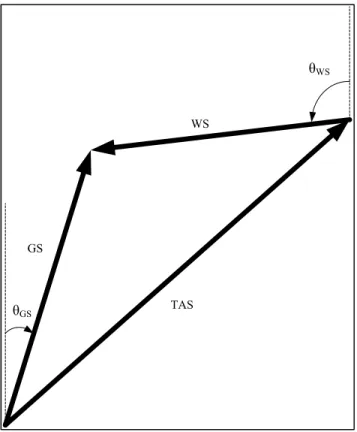
Normally though, the wind does not come directly from the tail or from the nose, but from different angles that change often during flight. In order to obtain the component of wind that pushes back or pulls forward the airplane, the wind vector has to be identified and decomposed in the longitudinal axis of the aircraft. This is not an easy task. In order to perform this decomposition, the wind triangle [26] is used which has been successfully implemented in [17][18][27]. Figure 3.2 shows the vectors involved in the wind triangle.
Figure 3.2 Wind triangle
By inspecting this figure, equations (3.3) – (3.5) can be written.
= + (3.3) = + (3.4) = + (3.5) TAS GS WS θGS θWS
Where TASx is the component in x axis and TASy is the component in y axis from the vector
TAS, WS is the wind speed, θGS is the angle to the destination point measured from the
magnetic north (azimuth) and θWS is the direction of the wind measured from the magnetic
north.
To obtain the GS, equations (3.4) and (3.5) are substituted in equation (3.3) obtaining a second degree equation (3.6) which can be easily solved using the general quadratic formula.
− 2( )( )( + ) + − = 0 (3.6)
3.4 Earth Model
In the algorithm presented in this work, it is important to always know the position of the aircraft with respect to the Earth. This is important to correctly estimate meteorological conditions and to measure the distance traveled by the aircraft. The parameters needed from the earth model are the coordinate of longitude, the coordinate of latitude and the azimuth. The azimuth can be defined as the angle that is formed between the aircraft and Magnetic North. Even though there are many different models of the earth, the ones examined in this thesis were the function legs, azimuth and track2 available with MATLAB and the equations of Vicenty implemented in two functions by Deakin in [28]. The MATLAB model and the equations of Vicenty provide the geodesic or great circle route. The geodesic route is the shortest curve between two points in a curved space such as the earth.
The function legs provides the distance between two points, the function track2 provides the coordinates of a great circle between two points and the function azimuth gives the azimuth between two points. Vicenty’s equations functions provide similar information as MATLAB functions. The two Vicenty’sfunctions are given by the direct and the inverse method. The direct method provides the coordinates where the aircraft is located after traveling a given distance in a given direction. The inverse method gives the distance between two points and the initial azimuth by providing the initial and last points.
33
The difference between these methods is the information that they need and the outputs that they can provide. Table 3.1 describes the Vicenty’s equations methods.
Table 3.1 Vicenty’s methods descriptions
Direct Method
Input Initial latitude (º), initial longitude (º), initial azimuth (º) and distance (meters) Output Final latitude (º), final longitude (º)
Inverse Method
Input Initial latitude (º), initial longitude (º), final latitude (º) and final longitude (º) Output Distance between points (meters), initial azimuth (º).
The formulation of these methods and the equations that describe them are explained by Gagné [18] and their complete development can be found in [28].
The Earth model selected for the algorithm is the one provided by the methods derived by Vicenty’s equations. The reasons are that only 2 functions are needed instead of the three needed by the MATLAB model. Therefore, when the cost computation of the airplane trajectory is computed, the aircraft model gives the distance traveled to perform a task, e.g. horizontal distance traveled during a climb. The coordinates where the aircraft will be found are easily obtained using the direct method. The azimuth is found by using the inverse method. Only two functions are needed.
3.5 Weather model
The ISA is a good way of testing and developing algorithms and it is used to develop many different aeronautical technologies. However, for trajectory optimization it is not the most adequate model because real flights do not take place in conditions where the meteorological variables are standard and where winds are non-existent. Thus, a different meteorological model is needed to calculate trajectories for real flights. The current FMS from CMC Electronics - Esterline accepts up to 4 points in which meteorological data can be manually
introduced. This information is limited and it is not enough to search for alternative routes or to calculate the complete effect of weather in the flight cost. The obtainment of more meteorological information allows a better choice of a VNAV trajectory by searching the altitude with the best combination of temperature and wind. It also allows searching alternative lateral routes depending on the wind and temperature variations.
To obtain a precise model of the atmosphere, the global forecast from Environment Canada is used. This model provides meteorological information all around the Earth in the form of a grid. Every vortex that is shown in Figure 3.3 contains meteorological information [30]. This model is used because is precise, widely popular in North America, freely available and it has been successfully implemented in two other projects at LARCASE giving good results.
Figure 3.3 Global coverage of Environment Canada forecast Source: Environment Canada
3.5.1 GRIB2 description
The information provided in this model is in the form of General Regularly-distributed Information in binary form version 2 (GRIB2). The GRIB2 files provide different information, but not all of it is needed by the algorithm. The needed information to perform our trajectory computation is available in the GRIB2 files that contain the data described in Table 3.2.
35
Table 3.2 GRIB2 variables needed in the algorithm
Variable Variable Name Units
TMP Temperature Kelvin
WDIR Wind direction Degrees
WIND Wind speed Knots
HGT Geopotential altitude Meters MSL Sea level pressure Pascal
Firstly, this data has to be downloaded from Internet. Because many files have to be downloaded, a small script in Matlab was used to download the files automatically using the software wget [29]. The downloaded files have the following nomenclature [30]:
CMC_glb_Variable_LevelType_Level_projection_YYYYMMDDHH_Phhh.grib2
The meaning of each part of the file is described in Table 3.3. Time is in Coordinated Universal Time (UTC).
Table 3.3 GRIB2 file nomenclature
Chain Segment Meaning
CMC Canadian meteorological centre
_glb GEM-GDPS Model
_Variable Variable from Table 3.3 described in the file _LevelType Variable data at this Isobaric level
_Level Isobaric level
_Projection Projection used for the data. Latlon or polar. Latlon is the one used _YYYYMMDD Year, month and day of prediction
HH Prediction time. Available every 3 hrs from hr 0 to gr 144 Phhh P is a constant character and hhh the forecast hour