Exploring Time-Varying Jump Intensities: Evidence from S&P500 Returns and Options

Texte intégral

(1)2009s-34. Exploring Time-Varying Jump Intensities: Evidence from S&P500 Returns and Options Peter Christoffersen, Kris Jacobs, Chayawat Ornthanalai. Série Scientifique Scientific Series. Montréal Août 2009. © 2009 Peter Christoffersen, Kris Jacobs, Chayawat Ornthanalai. Tous droits réservés. All rights reserved. Reproduction partielle permise avec citation du document source, incluant la notice ©. Short sections may be quoted without explicit permission, if full credit, including © notice, is given to the source..

(2) CIRANO Le CIRANO est un organisme sans but lucratif constitué en vertu de la Loi des compagnies du Québec. Le financement de son infrastructure et de ses activités de recherche provient des cotisations de ses organisations-membres, d’une subvention d’infrastructure du Ministère du Développement économique et régional et de la Recherche, de même que des subventions et mandats obtenus par ses équipes de recherche. CIRANO is a private non-profit organization incorporated under the Québec Companies Act. Its infrastructure and research activities are funded through fees paid by member organizations, an infrastructure grant from the Ministère du Développement économique et régional et de la Recherche, and grants and research mandates obtained by its research teams. Les partenaires du CIRANO Partenaire majeur Ministère du Développement économique, de l’Innovation et de l’Exportation Partenaires corporatifs Banque de développement du Canada Banque du Canada Banque Laurentienne du Canada Banque Nationale du Canada Banque Royale du Canada Banque Scotia Bell Canada BMO Groupe financier Caisse de dépôt et placement du Québec DMR Fédération des caisses Desjardins du Québec Gaz de France Gaz Métro Hydro-Québec Industrie Canada Investissements PSP Ministère des Finances du Québec Power Corporation du Canada Raymond Chabot Grant Thornton Rio Tinto State Street Global Advisors Transat A.T. Ville de Montréal Partenaires universitaires École Polytechnique de Montréal HEC Montréal McGill University Université Concordia Université de Montréal Université de Sherbrooke Université du Québec Université du Québec à Montréal Université Laval Le CIRANO collabore avec de nombreux centres et chaires de recherche universitaires dont on peut consulter la liste sur son site web. Les cahiers de la série scientifique (CS) visent à rendre accessibles des résultats de recherche effectuée au CIRANO afin de susciter échanges et commentaires. Ces cahiers sont écrits dans le style des publications scientifiques. Les idées et les opinions émises sont sous l’unique responsabilité des auteurs et ne représentent pas nécessairement les positions du CIRANO ou de ses partenaires. This paper presents research carried out at CIRANO and aims at encouraging discussion and comment. The observations and viewpoints expressed are the sole responsibility of the authors. They do not necessarily represent positions of CIRANO or its partners.. ISSN 1198-8177. Partenaire financier.

(3) Exploring Time-Varying Jump Intensities: Evidence from S&P500 Returns and Options* Peter Christoffersen †, Kris Jacobs‡, Chayawat Ornthanalai § Résumé Les recherches empiriques standards portant sur la dynamique des sauts dans les rendements et dans la volatilité sont plutôt complexes en raison de la présence de facteurs inobservables en temps continu. Nous présentons un nouveau cadre d’étude en temps discret qui combine des processus hétéroscédastiques et des caractéristiques à concentration élevée de sauts dans les rendements et dans la volatilité. Nos modèles peuvent être facilement évalués à l’aide des méthodes standards du maximum de vraisemblance. Nous offrons une démarche souple de neutralisation du risque pour cette catégorie de modèles, ce qui permet de modéliser distinctement les primes de risque liées aux sauts et celles liées aux innovations normales. Nous imbriquons nos modèles dans la littérature en établissant leurs limites en temps continu. Ces derniers sont évalués en intégrant un échantillon de rendements à long terme de l’indice S&P 500 et en évaluant un vaste échantillon d’options. Nous trouvons un solide appui empirique en ce qui a trait aux intensités de sauts variant dans le temps. Un modèle avec intensité de saut affine dans la variance conditionnelle est particulièrement efficace sur les plans de l’ajustement des rendements et de l’évaluation des options. La mise en œuvre de notre modèle permet de multiples sauts par jour et les données appuient cette caractéristique, plus particulièrement en ce qui a trait au lundi noir d’octobre 1987. Nos résultats confirment aussi l’importance des primes liées au risque de sauts pour l’évaluation du prix des options : les sauts ne peuvent contribuer à améliorer considérablement la performance des modèles utilisés pour fixer les prix des options, sauf en présence de primes de risque de sauts assez importantes. Mots clés : processus composé de Poisson, évaluation du prix des options, filtrage, sauts liés à la volatilité, primes de risque de sauts, intensité des sauts variant dans le temps, hétéroscédasticité.. *. P. Christoffersen and K. Jacobs are grateful for financial support from FQRSC, IFM2 and SSHRC. P. Christoffersen gratefully acknowledges the hospitality of CBS and the financial support from the Center for Research in Econometric Analysis of Time Series, CREATES, funded by the Danish National Research Foundation. Ornthanalai was supported by CIREQ and J.W. McConnell Fellowships. We would like to thank the participants at EFA, EFMA, the FDIC Derivatives Conference and the Canadian Econometrics Study Group for helpful comments. Any remaining inadequacies are ours alone. † Corresponding author: McGill University, CREATES, CIRANO and CIREQ. Desautels Faculty of Management, McGill University, 1001 Sherbrooke Street West, Montreal, Quebec, Canada, H3A 1G5; Tel: (514) 398-2869; Fax: (514) 398-3876; E-mail: peter.christoffersen@mcgill.ca. ‡ McGill University, Tilburg University, CIRANO and CIREQ. §. McGill University..

(4) Abstract Standard empirical investigations of jump dynamics in returns and volatility are fairly complicated due to the presence of latent continuous-time factors. We present a new discretetime framework that combines heteroskedastic processes with rich specifications of jumps in returns and volatility. Our models can be estimated with ease using standard maximum likelihood techniques. We provide a tractable risk neutralization framework for this class of models which allows for separate modeling of risk premia for the jump and normal innovations. We anchor our models in the literature by providing continuous time limits of the models. The models are evaluated by fitting a long sample of S&P500 index returns, and by valuing a large sample of options. We find strong empirical support for time-varying jump intensities. A model with jump intensity that is affine in the conditional variance performs particularly well both in return fitting and option valuation. Our implementation allows for multiple jumps per day, and the data indicate support for this model feature, most notably on Black Monday in October 1987. Our results also confirm the importance of jump risk premia for option valuation: jumps cannot significantly improve the performance of option pricing models unless sizeable jump risk premia are present. Keywords: compound Poisson process, option valuation, filtering; volatility jumps, jump risk premia, time-varying jump intensity, heteroskedasticity. Codes JEL : G12.

(5) 1. Introduction. This paper provides a modeling framework that allows for general specifications and easy maximum likelihood estimation of jump models using asset returns. Our framework allows for correlated jumps in returns and volatility, as well as time-varying jump intensities, which may be characterized by a separate dynamic. Our models also allow for time-varying variance of the normal innovation as well as time-varying jump intensity of the jump innovation. We allow for multiple jumps each day and we suggest a filtering technique to identify these jumps. We provide the risk-neutral processes for use in option valuation and we develop continuous time limits of our discrete time models. Our framework has certain advantages. First and foremost, the implementation of our framework is facilitated by the fact that we use a discrete-time approach, and by the way in which we model the time-variation in the jump intensity. As suggested in Fleming and Kirby (2003), we directly use GARCH processes as filters for the unobservable state variables. As a result, various specifications of complex jump models can be estimated on return data using a standard MLE procedure. Second, because filtering is relatively straightforward, we do not need to approximate the compound Poisson process as a Bernoulli process, which is a common practice in several continuous-time studies. We therefore allow for the possibility that there is more than one jump per time period. We find strong evidence of this, particularly on Black Monday in October 1987. Third, we can separate the risk premia associated with the jump and the normal innovation. This follows from our risk-neutralization procedure, which in this way differs from existing approaches. A fourth potential advantage of our GARCH specification as compared to a (continuous-time or discrete-time) stochastic volatility specification is that all parameters needed for option valuation can be obtained from estimation on returns only. We estimate four different but nested models. The simplest model, which we label DVCJ (dynamic volatility with constant jumps), has a constant jump intensity. This model is closely related to the most popular model in the continuous-time literature, the stochastic volatility with correlation jumps (SVCJ) model, which is studied among others by Eraker, Johannes, and Polson (EJP, 2003), Li, Wells and Yu (2007), Chernov, Gallant, Ghysels and Tauchen (CGGT, 2003) and Eraker (2004). The CVDJ (constant volatility with dynamic jumps) has a time-varying jump intensity, but the normal innovation to the return process is assumed to be homoskedastic. The DVSDJ (dynamic volatility with separate dynamic jump) model is the most general model we investigate: both the jump and the normal innovation are timevarying, and the dynamics are separately parameterized. In this case, the jump intensity carries its own GARCH dynamic. The DVDJ (dynamic volatility with dynamic jumps) model is a special case of DVSDJ: both the jump and the normal innovation are time-varying, but parameterized identically. To further relate our models to the available literature, Table 1 provides an overview of some existing empirical studies studying finite-activity jump processes, and indicates how the four models we propose are related to this literature. The bottom panel of Table 1 indicates that our four models can accommodate the mechanics of various complex jump specifications currently used in the literature. Our approach is perhaps most closely related to the discretetime approach in Maheu and McCurdy (2004). They find strong evidence of time-varying jump intensities in individual equity returns. We find similar evidence using equity index returns, and importantly we provide theory and empirics on option valuation using our jump models. Duan, Ritchken and Sun (2006) also provide risk neutralization of a GARCH model 2.

(6) with jumps, but they do not allow for time-varying jump intensities. Table 1 also indicates that the most complex specifications we propose, the DVDJ and DVSDJ models, are closely related to the most complex dynamics investigated in the continuoustime literature. By providing models with complex dynamics that are straightforward to implement, we are able to contribute to the growing but still limited literature on time-varying jump intensities. In particular, our estimates using return data can be directly related to the findings of Bates (2006), and Andersen, Benzoni and Lund (ABL, 2002), who estimate models that allow for state-dependent jump intensities. Bates (2000), Pan (2002), Eraker (2004), and Huang and Wu (2004) also allow for state-dependent jump intensities but they use options to help extract the latent volatility process instead of directly filtering them from the underlying return. Because implementation of our models is straightforward, we are also able to estimate models with characteristics that have hitherto not been estimated in the literature. In particular, we estimate models with time-varying jump intensities and jumps in volatility, while allowing for multiple jumps per day, and we are able to estimate these models while explicitly solving the filtering problem using long time series of returns. Our empirical investigation estimates the four models we propose using twenty years of daily S&P500 returns, from 1985 through 2004. After estimating these processes using returns data, we risk-neutralize them and compare their option valuation performance using nine years of index call option data from 1996 through 2004. The empirical results on returns and options allow us to address a number of important questions. (1) How should jump and normal (diffusive) innovations be jointly modeled in equity index returns? (2) Are jump intensities time-varying for the purpose of option valuation? (3) Do the data favor a specification that allows for more than one jump per day? How does this assumption impact on the evidence regarding time-varying jump intensity? (4) Do we need jump risk premia to model index option prices? (5) Are jumps needed for option valuation at all times or only in certain regimes? Finally, we also extract the time-series of conditional variance for jump and normal components. This allows us to address the following question (6) How large is the jump component and how much does it vary over time? With regard to (1), we find that models without heteroskedasticity in the normal innovation are severely misspecified, which is entirely consistent with the continuous-time literature. Both the return-based and option-based evidence support the presence of jumps in returns as well as jumps in volatility. Our jump parameter estimates are roughly consistent with the results of Eraker (2004), EJP (2003), ABL (2002), and CGGT (2003). With regard to (2), our MLE estimates show strong support for the DVDJ model, with time-varying jump intensities and linear dependence on the variance of the normal innovation. Under this specification, we obtain up to 17% improvement in the implied volatility root mean squared option pricing errors over the simple GARCH case. The DVDJ model is comparable to the continuous-time SVSCJ model. While to our knowledge time-series-based estimation of the SVSCJ model is not available in the literature, ABL (2002) use a model without volatility jumps and find no time-series based evidence for a time-varying intensity. Bates (2006) estimates this model using the same data set and finds evidence for time-varying jump intensity. ABL (2002) and Bates (2006) are, to our knowledge, the only two papers that estimate jump models with time-varying intensity on returns. Our results are therefore more supportive of time-varying intensities than the available literature, but it must be noted that due to the GARCH filter, jumps in return and volatility are perfectly correlated. The strong correlation between return and volatility jumps is supported by Todorov and Tauchen (2008) 3.

(7) who examine high frequency S&P500 and VIX data. They find strong dependence between realized jumps in the two series. Regarding (3), our estimates support the presence of multiple jumps per day in the October 1987 period. We speculate that not allowing for this possibility has biased existing studies against detecting time-varying jump intensities. For (4), we find that in order to produce significant improvements in option valuation, jump models must allow for jump risk premia. We investigate if risk premia for the jump and the normal innovation can generate the various shapes and levels of the implied volatility term structure, and we find that the implied volatility term structure is highly responsive to the level of the jump risk premium. On the other hand, unrealistically large magnitudes of risk premia for the normal innovation are required in order to generate levels and slopes of implied volatility comparable to the data. Therefore, we conclude that jump risk premia are necessary for realistic modeling of option prices. Regarding question (5), we conclude that jump models provide superior option pricing performance during the medium to high volatility periods, but jumps do not help when the VIX index is well below its average. Finally, regarding (6), we find that the contribution of the jump component to total equity volatility is between 15 and 75 percent, depending on the model. The remainder of the paper proceeds as follows. Section 2 presents our modeling approach and discusses the four nested specifications. Section 3 provides the empirical results from estimating the models on daily returns. Section 4 develops the theoretical framework for risk-neutralization and option valuation. Section 5 provides the empirical results on option valuation. Section 6 develops continuous time limits of our models and provides a filtration of the jump and normal components. Section 7 concludes.. 2 2.1. Daily Returns with Jump Intensity Dynamics The Return Process. In this section, we present the general return dynamic. This dynamic contains two components. The first is the component which corresponds to the diffusive term in continuous-time setups. Because we model this component using a normal innovation, we will henceforth refer to it as the normal component. The second is the jump component. Here we discuss some aspects of the structure of the jump and normal components, and we postpone the specifications of the time-variation in their conditional variance until Section 2.3. The return process is given by ¶ µ ¡ ¢ St+1 Rt+1 ≡ log = r + λz − 12 hz,t+1 + (λy − ξ) hy,t+1 + zt+1 + yt+1 , (2.1) St. where St+1 denotes the underlying asset price at the close of day t + 1, and r the risk free rate. Shocks to returns are generated by the normal component zt+1 and the pure jump component yt+1 , which are assumed to be contemporaneously independent. The normal component zt+1 is assumed to be distributed N (0, hz,t+1 ) , where hz,t+1 is the conditional variance. We model the jump component using the compound Poisson process, which is the standard jump process used in the continuous-time literature. See Merton (1976) for an early treatment of these processes ¡ ¢ in finance. We let yt+1 be conditionally distributed as compound 2 Poisson J hy,t+1 , θ, δ , where hy,t+1 denotes the jump intensity (or jump arrival rate), θ the 4.

(8) mean jump and´δ 2 the jump size variance. The convexity adjustment terms 12 hz,t+1 and ³ size, δ2 ξhy,t+1 ≡ eθ+ 2 − 1 hy,t+1 in (2.1) act as compensators to the normal and jump component respectively. Thus, when taking conditional expectations of the gross rate of return, we get ∙ ¸ St+1 = er+λz hz,t+1 +λy hy,t+1 , (2.2) Et St which shows that γ t+1 ≡ λz hz,t+1 + λy hy,t+1 is the conditional equity premium, with λz and λy the market prices of risk for the normal and jump components respectively. Our setup allows for the possibility of time-varying equity premia, and these dynamics will depend on the specification of hz,t+1 and hy,t+1 . Our specification in (2.1) is similar in spirit to the return process of Heston and Nandi (2000), with the addition of a jump component. Barone-Adesi, Engle and Mancini (2008) propose a nonparametric approach to model conditionally non-normal innovations. Maheu and McCurdy (2004, 2008) study similar return processes with jumps but do not provide the risk-neutral process, which is necessary for option valuation. Duan, Ritchken, and Sun (2006, 2007) propose return dynamics similar to (2.1), and provide risk-neutralization arguments, but their setup differs from ours in important ways. First, we use a different specification of the equity premium. Our specification of the equity premium is affine in the state variables, which has several advantages. The affine specification greatly facilitates the comparison with standard continuous time models that we undertake in Section 6. We also use the affine structure in order to separate the jump and diffusive risk premia, and it also makes it relatively straightforward to derive the risk-neutral dynamic, which is crucial for option pricing. Second, Duan, Ritchken and Sun (2006, 2007) consider processes without time-varying jump intensities. Third, in our specification jump and normal components carry independent risk premia. Fourth, and most importantly, the conditional skewness and kurtosis in Duan, Ritchken and Sun (2006, 2007) are constant through time, whereas this is not the case in our specification, as we will demonstrate in Section 2.5.. 2.2. The Structure of the Jump Innovation. The compound Poisson structure assumes that the jump size is independently drawn from a normal distribution with mean θ and variance δ 2 . The number of jumps nt+1 arriving between times t and t + 1 is a Poisson counting process with intensity hy,t+1 . The jump component in the period t + 1 return is therefore given by yt+1 =. nP t+1 j=0. xjt+1. where xjt+1¡, j =¢ 0, 1, 2, ... is an i.i.d. sequence of normally distributed random variables with xjt+1 ∼ N θ, δ 2 . The conditional expectation of the number of jumps arriving over the time interval (t, t + 1) equals the jump intensity, Et ¡[nt+1 ] =¢hy,t+1 . The mean and variance of the jump component, yt+1 , are given by θhy,t+1 and δ 2 + θ2 hy,t+1 respectively. Intuitively, hy,t+1 should be time-varying as the number of jumps occurring at any time period will depend on market conditions. Unfortunately, jump models with time-varying jump intensity are difficult to estimate and implement in continuous-time models with latent factors, because the 5.

(9) likelihood function typically is not available in closed form. The filtration procedure for the latent jump and stochastic volatility processes is also far from straightforward in continuous time. Therefore, the literature contains limited evidence on equity returns and option pricing models with stochastic jump intensity. The filtration problem in our setup is a lot more straightforward. We will test several specifications for hy,t+1 , ranging from the simple case of a constant arrival rate to modeling it using a separate GARCH dynamic.. 2.3. The Heston and Nandi GARCH(1,1) Benchmark Model. Heston and Nandi (2000) propose a class of GARCH models that allow for a closed-form solution for European options. The GARCH(1,1) version of this model is given by p ¡ ¢ (2.3) Rt+1 = r + λz − 12 hz,t+1 + hz,t+1 εt+1 ³ ´ 2 p hz,t+1 = wz + bz hz,t + az εt − cz hz,t. where r is the risk free rate, and εt+1 is the innovation term distributed i.i.d. N (0, 1). The variance of the return is hz,t+1 . The asymmetric variance response, or the leverage effect, is captured by the parameter cz . This model is based on conditional normality and thus cannot generate one-period-ahead conditional skewness and excess kurtosis. The GARCH dynamic in (2.3) is different from the more conventional NGARCH model used by Engle and Ng (1992) and Hentschel (1995), which is used by Duan (1995) to price options. We choose the GARCH dynamic (2.3) as our benchmark since it ensures the closest possible correspondence of our jump parameter estimates with the continuous-time literature. Our objective is to present a general approach that can be applied to any dynamics, and we leave the determination of the preferred dynamics in the presence of joint normality and compound Poisson jumps for future research. Before we extend the Heston-Nandi framework p to the returns process in (2.1), we rewrite the GARCH(1,1) dynamic in (2.3). Letting zt+1 = hz,t+1 εt+1 , we get ¡ ¢ Rt+1 = r + λz − 12 hz,t+1 + zt+1 az hz,t+1 = wz + bz hz,t + (zt − cz hz,t )2 . hz,t The unconditional variance is given by E [hz,t+1 ] = (wz + az ) / (1 − bz − az c2z ) , where bz +az c2z is the variance persistence. We will use the empirical performance of the Heston-Nandi model as a benchmark for the evaluation of our proposed jump models. Because we only use the GARCH(1,1) implementation, we henceforth refer to it simply as the GARCH model.. 2.4. Four Nested Models. We now apply the simple Heston-Nandi GARCH dynamic to the two return innovations in (2.1). We will refer to these two dynamics as the conditional variance (for the normal component) and the time-varying jump intensity (for the jump component). For the most general specification, both the jump intensity and the variance of the normal. 6.

(10) innovation are governed by a Heston-Nandi type GARCH(1,1) dynamic. az (zt + yt − cz hz,t )2 hz,t ay = wy + by hy,t + (zt + yt − cy hy,t )2 hy,t. hz,t+1 = wz + bz hz,t +. (2.4). hy,t+1. (2.5). The subscripts z and y are applied to distinguish the parameters governing the dynamic of hz,t+1 and hy,t+1 respectively. In (2.4)-(2.5), the dynamics of hz,t+1 and hy,t+1 are predictable conditional on information available at time t, and it is the total return innovation, zt + yt , observable at time t, that generates the variance and jump intensity one period ahead. The specification therefore implies jumps in volatility, which are supported by the empirical findings of Broadie, Chernov and Johannes (BCJ, 2007), Eraker (2004) and EJP (2003). In a continuous-time setting, adding jumps to stochastic volatility models involves an additional set of latent state variables. The study of option pricing in stochastic volatility models with jumps therefore relies heavily on econometric methods that can filter the unobserved state variables. CGGT (2003) use an EMM based method, Pan (2002) uses the implied-state GMM technique to fit her models to returns and option prices, while EJP (2003), Eraker (2004) and Li, Wells, and Yu (2007) employ MCMC techniques. In comparison, our use of GARCH models in (2.4)-(2.5) is computationally convenient, because the GARCH model serves as a simple filter where the state variables hz,t+1 and hy,t+1 are directly computed from the observed shocks, and therefore all of our models can be estimated from returns data using a standard Maximum Likelihood technique. We investigate four nested models based on the general dynamic in (2.4)-(2.5). Similar to Huang and Wu (2004), our models generate time-varying higher moments of returns from the variance of the normal component hz,t+1 and/or from the jump intensity hy,t+1 . We now present these four specifications. The Dynamic Volatility and Constant Jumps (DVCJ) Model The first specification we explore is akin to the most common specification in the continuoustime affine jump diffusion literature, namely the stochastic volatility with correlated jumps (SVCJ) model studied by EJP (2003), CGGT (2003), Li, Wells and Yu (2007), and Eraker (2004). Compared to our most general specification (2.4)-(2.5), we turn off the time-varying jump intensity dynamic while maintaining the normal component’s GARCH dynamic. This amounts to the restrictions by = 0 ay = 0 cy = 0. The DVCJ model contains nine parameters, three more than the Heston-Nandi model. In any given period, the DVCJ model implies that jumps arrive at a constant rate of wy , regardless of the level of volatility in the market. Although this may seem counter-intuitive, it is assumed in most of the existing literature. The Constant Volatility and Dynamic Jumps (CVDJ) Model The CVDJ model allows for jump dynamics but turns off the dynamic in the conditional variance of the normal component. It is a special case of the general dynamic in (2.5), with the restrictions bz = 0 az = 0 cz = 0. 7.

(11) In this specification, time-variation in returns is driven by the jump component. The normal component of returns is homoskedastic, with the variance equal to wz . This is equivalent to applying stochastic time change only to the pure jump process in Carr, Geman, Madan and Yor (2003) and Carr and Wu (2004). Given that time variation is restricted to the jump intensity, we expect to see an increase in the relative importance of the jump component in returns for this specification. The Dynamic Volatility and Dynamic Jumps (DVDJ) Model The DVDJ specification can be written as a special case of the most general specification, subject to the following restrictions on the parameters of hy,t+1 in (2.5) wy = wz k. ay = az k 2. by = bz. cy =. cz k. In the DVDJ specification hz,t+1 and hy,t+1 are both time-varying but driven by the same dynamic. We specify the jump intensity to be affine in the conditional variance of the normal component hy,t+1 = khz,t+1 (2.6) where k is a parameter to be estimated. The affine structure (2.6) is studied in a continuoustime setting by Bates (2000, 2006), Eraker (2004), ABL (2002), Huang and Wu (2004), and Pan (2002). Table 1 indicates that some of these papers estimate this model using returns data, and others using options data. Overall, the evidence on time-varying jump intensities is mixed. Estimating on option data, Bates (2000) does not find evidence of time-varying jump intensities, but Pan (2002) and Eraker (2004) do find statistically significant estimates for k by fitting their models to option data. Using return data, ABL (2002) do not find evidence of time varying jump intensities, but Bates (2006) does. These different findings may be due to differences in model specification and/or estimation technique. Eraker (2004) estimates his model using MCMC and specifies correlated jumps in returns and volatility. ABL (2002) use EMM to estimate models with jumps in returns only. Bates (2000) and Pan (2002) do not estimate models with jumps in volatility. Given these differences in model specification in the continuous-time literature, it is worth keeping in mind that the closest continuous-time counterpart of the DVDJ model is the SVSCJ model, which stands for stochastic volatility with state-dependent, correlated jumps.1 The only paper that estimates this model is Eraker (2004). The SVSCJ is the most general model considered by Eraker (2004), who finds it outperforms other models when simultaneously fitting option data and S&P500 index returns. The Dynamic Volatility and Separate Dynamic Jumps (DVSDJ) Model We refer to the most general specification, where the conditional variance of the normal component and the jump intensity are governed by separate processes, as the DVSDJ model. Since the two variance components vary over time, their relative contribution to returns will also be time-varying. Separate dynamics also allow the variance components to mean-revert 1. The DVDJ model is a special case of the most general SVSCJ, because jumps in returns and volatility are perfectly correlated in the GARCH setting.. 8.

(12) at different rates. This is empirically relevant, because Eraker (2004) and Huang and Wu (2004) provide evidence that shocks from jump components are more persistent and decay at a slower rate than the shock associated with the normal innovation. The DVSDJ model is related to the continuous-time models estimated by Huang and Wu (2004) and Santa-Clara and Yan (2008). Similarly to the DVSDJ model, in those specifications the time-varying jump intensity has its own separate dynamic, rather than being a simple linear function of another state variable. However, these specifications differ from DVSDJ in the sense that the time-varying jump intensity contains a separate shock. We therefore refer to these specifications as “stochastic jump intensities” in Table 1. We choose the DVSDJ specification because of the resulting econometric advantages. Finally, note that the DVSDJ model is more complex than similar available continuous-time models in another sense, because it allows for jumps in volatility. Huang and Wu (2004) estimate a continuous-time specification similar in spirit to (2.4)(2.5) using European options on the S&P500 index, and find that it outperforms other models both in and out-of-sample. However, their result is based on minimizing option pricing errors over a short period, and the time series of underlying returns does not enter their objective function. Santa-Clara and Yan (2008) also estimate a related model using a technique similar to that used by Pan (2002), where at each point in time the state variables are inferred directly from option data. To the best of our knowledge, the literature does not contain estimates for a continuous-time model akin to (2.4)-(2.5) based on returns data. This is perhaps due to the large number of latent factors. This renders the likelihood function unavailable, which in turn makes the estimation much more challenging. Our discrete-time setup and the convenient GARCH filtration allow us to estimate the DVSDJ model using standard MLE techniques.. 2.5. Conditional Moments of Returns. Conditional moments of returns can be readily derived using the moment generating function of the normal and compound Poisson processes. The first four conditional moments are ¡ ¢ Et (Rt+1 ) ≡ μt+1 = r + λz − 12 hz,t+1 + (λy − ξ + θ) hy,t+1 ¡ ¢ V art (Rt+1 ) = hz,t+1 + δ 2 + θ2 hy,t+1 ¢ ¡ θ 3δ 2 + θ2 hy,t+1 Skewt (Rt+1 ) = ¡ ¢ ¢3/2 ¡ hz,t+1 + δ 2 + θ2 hy,t+1 ¢ ¡ 4 3δ + 6δ 2 θ2 + θ4 hy,t+1 Kurtt (Rt+1 ) = 3 + ¡ ¡ ¢ ¢2 hz,t+1 + δ2 + θ2 hy,t+1. (2.7) (2.8) (2.9) (2.10). where Skewt (Rt+1 ) is the conditional skewness of returns, and Kurtt (Rt+1 ) is the conditional kurtosis. The sign of the conditional skewness depends on the sign of the mean jump size θ. For positive hy,t+1 , which means in the presence of jumps, the dynamics of conditional skewness and kurtosis are driven by the conditional variance of the normal component as well as the jump intensity. Harvey and Siddique (1999, 2000) document the importance of timevarying skewness in asset pricing. The time-variation in conditional skewness and kurtosis is a critical difference between our approach and the framework in Duan, Ritchken and Sun (2006,. 9.

(13) 2007), in which conditional skewness and kurtosis are constant through time. Expressions for variance persistence and for the long run variance of all four models are provided in Appendix A.. 2.6. The Likelihood Function. The likelihood function for returns depends on the normal and Poisson distributions. First, notice that conditional on nt+1 = j jumps occurring in a period, the conditional density of returns is normal µ ¶ 2 (Rt+1 −μt+1 −jθ) exp − 2 h ( z,t+1 jδ2 ) (2.11) ft (Rt+1 |nt+1 = j) = q ¡ ¢ , 2π hz,t+1 + jδ 2 Because the number of jumps is finite in the compound Poisson process, the conditional probability density of returns can be derived by summing over the number of jumps, which is distributed as a Poisson counting process Prt (nt+1. (hy,t+1 )j exp (−hy,t+1 ) . = j) = j!. (2.12). This yields the conditional density in terms of the observables ft (Rt+1 ) =. ∞ P. j=1. ft (Rt+1 |nt+1 = j) Prt (nt+1 = j) .. (2.13). and the likelihood function can now be constructed easily as the product of the conditional distributions across the sample. When implementing the maximum likelihood estimation, the summation (2.13) must be truncated. Most existing evidence indicates that jumps of the Poisson type are large and rare, with on average one to two jumps per year. However, we want to allow for the possibility of clustering of several jumps on a day. We therefore truncate the summation at 50 jumps per day. This truncation limit is twice the value used in Maheu and McCurdy (2004), because in our empirical work we find evidence of up to 16 jumps on a single day. Through experimentation, we have found that our estimation results are robust to setting the truncation higher than 50.. 3 3.1. Daily Return Empirics Data and Method. We estimate the models using the time series of S&P500 returns from January 1, 1985 through December 31, 2004. The data are obtained from CRSP. The top panel of Figure 1 shows the daily logarithmic return on the S&P500 for our sample. Several large or “jump-like” movements in returns are apparent. The largest price change is the crash of October 1987, when the index falls by almost 25 percent in a single day. We use a long sample of returns because it is well-known that it is difficult to estimate GARCH parameters precisely using relatively short samples. Even more importantly, jumps are rare events, and given an average 10.

(14) occurrence of one or two jumps per year estimated in the existing literature, it is difficult to get sensible estimates on jump parameters with daily return data that spans less than ten to fifteen years. We estimate the models using standard Maximum Likelihood. For updating the variance dynamic, we use starting values that correspond to the model-implied long-run jump intensity and the long-run variance. That is, we set hz,1 = E [hz,t ] ≡ σ 2z and hy,1 = E [hy,t ] ≡ σ 2y . The optimization converges quickly and the estimates are robust to a wide range of starting values.. 3.2. Maximum Likelihood Estimates. Table 2 presents Maximum Likelihood estimates (MLE) for the four proposed jump models, obtained using returns data for 1985-2004. For reference, Table 3 presents MLE estimates for three benchmark models, namely the Heston and Nandi (2000) model, the Black and Scholes (1973) model, and the Merton (1976) jump model. For each model, we divide parameter estimates into two columns, one for parameters representing the normal component, and the other for parameters representing the jump component. For example, the parameter λ in the “Jump” column refers to the λy parameter. Under each parameter estimate, we report its robust standard error calculated from the outer product of the gradient at the optimum parameter value. Using only returns data, it is difficult to simultaneously obtain precise estimates of the market prices of jump and normal risks. We therefore assume that in our jump models, λz = 0. This assumption is similar to the one used in Pan (2002) who estimates options and returns of the S&P500 jointly. She finds that neither the diffusion nor the volatility risk premia in her model are statistically significant, and specifically constrains the volatility risk premium to be zero.2 BCJ (2007) estimate the risk premia in the S&P500 index options using the SVCJ model and find a negligible value for the volatility risk premium. The effects on option valuation of different risk premium specifications will be analyzed in detail in Section 5. The log-likelihood values in Tables 2 and 3 show that all jump models in Table 2 significantly improve on the fit of the GARCH model in Table 3. Not surprisingly, the CVDJ model which has constant conditional variance of the normal component performs the worst among the jump models. Using the MLE estimates, we can recover the long run (unconditional) equity premium implied by each model. We report the values of the implied long run equity premium in the bottom row of Tables 2 and 3. The long run equity premium implied by the models ranges from 4.14% (DVCJ) to 7.98% (BSM) per annum. For our sample period, the realized return on the S&P500 in excess of the 3-month Treasury bill is approximately 5.74%. We can also compare our estimates of the models’ implied equity premium to the existing literature.3 Available estimates differ depending on the concepts, method, and data used in the calculations. Estimates of the historical equity return as reported in Ibbotson Associates (2006) range from 4.9 to 8.5%. Welch (2000) surveys finance and economics academics’ estimates of the expected equity premium over the next 30 years. He reports an average arithmetic equity premium of 7% over T-bills. We thus conclude that all our models produce implied long run 2. In the GARCH framework, the normal shocks in returns and volatilities are identical. As a result λz can also be thought of as the market price of volatility risk. 3 The literature on the equity premium is too large to cite in full here. See Cochrane (1997), Siegel and Thaler (1997), Mehra and Prescott (2003) and Fernandez (2006) for comprehensive surveys.. 11.

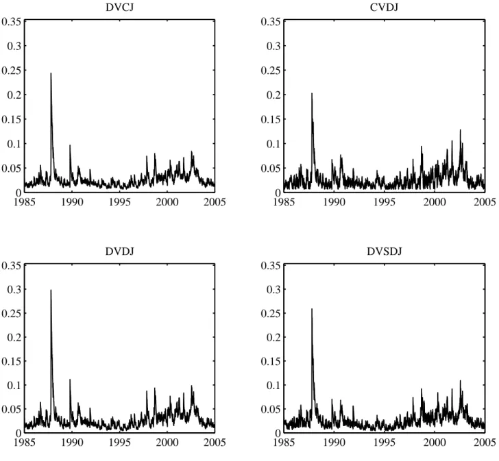
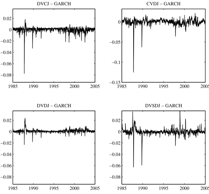
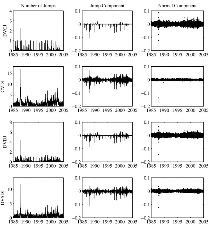
(15) equity premia that are reasonable given our sample period, and roughly consistent with the existing literature. Figure 2 shows the annualized conditional return variance for the four proposed jump models. We plot the total conditional variance defined above as ¡ ¢ V art (Rt+1 ) = hz,t+1 + δ 2 + θ2 hy,t+1. from January 1, 1985 through December 31, 2004. To aid the comparison with the conditional variance path of the GARCH model without jumps, we plot the difference between the conditional variance of each jump model and the Heston-Nandi model in Figure 3. Note that CVDJ has its own scale in Figure 3. As expected, the conditional variance paths look fairly similar across models in Figure 2. However, Figure 3 shows that important events such as the 1987 crash are captured quite differently across the models. The conditional normal GARCH model produces a very high conditional variance from the crash, whereas the jump models can allocate part of the crash to the higher moments. Figure 4 shows the jump intensity hy,t+1 over time for each model. It shows that the CVDJ specification has the largest magnitude of jump intensity in comparison with the other three proposed jump models. This is not surprising as jumps are the only source of heteroskedasticity in this model, and we therefore expect the jump component to be very volatile. Table 2 indicates that the size of the jumps arriving in the CVDJ model are also the smallest in comparison to other models, with a mean jump size of −0.110%, and a very high arrival rate. Consider now the DVCJ jump specification. Adding a simple constant jump component to a GARCH dynamic can significantly improve model fit, even though the variance parameters of the normal component in the DVCJ model are similar to those of the GARCH model. Table 2 reports a mean jump size of θ = −1.804%, and jump volatility of δ = 2.786%. As for the jump intensity E [hy,t+1 ] = wy , the model implies that jumps arrive at a frequency of 252 × wy ' 3.60 jumps per year. When compared with the estimates for the SVCJ model obtained by Eraker (2004) and EJP (2003), we find a somewhat smaller jump mean size and a somewhat higher jump intensity rate. This is not surprising as we allow for multiple jumps per day whereas the implementation in Eraker (2004) and EJP (2003) does not. The results for the DVDJ model indicate that allowing for state-dependent jump intensities can further improve model performance. The estimate of k is statistically significant, confirming that the arrival rate of jumps depends on the level of risk in the market. The mean jump size is smaller than for the DVCJ model. However, jumps arrive more frequently, with on average E [hy,t+1 ] = kσ 2z = 0.0644, or 16.2 jumps per year. When allowing for time-varying jump intensities, smaller jumps can occur at a frequency which depends on the level of risk in the market. The bottom-left panel in Figure 4 indeed shows considerable variation over time in the jump-intensity. Our evidence in support of time-varying jump intensities is in line with Eraker (2004) and Pan (2002), who estimate their models using joint information from returns and option prices. Bates (2006) also finds support for time-varying jump intensity from returns when estimating the model using his approximate maximum likelihood method, but his model does not include jumps in volatility. On the other hand, ABL (2002), estimating on returns, and Bates (2000), estimating on option prices, do not find evidence supporting time-varying intensities. The likelihood for the most general specification, DVSDJ, offers a sizable improvement over DVDJ. This illustrates the benefit of allowing for the jump intensity to be driven by its 12.

(16) own independent dynamic. The persistence of the jump intensity is approximately the same as the persistence of the variance of the normal component. Interestingly, for the DVSDJ model, we find that the estimate of the parameter cz , which controls the leverage effect in the variance of the normal component, is significantly negative. This is opposite to the intuition behind the “leverage effect” that drives asymmetry in the variance/return relationship. In other words, a positive normal shock to the return will increase the variance of the normal component by higher than a negative normal shock to the return. We conjecture that this result is due to the high level of negative skewness (left asymmetry) that is already produced by the jump component. Therefore, the heteroskedasticity in the normal component becomes an important factor in the modeling of the right tail of the return distribution. The MLE estimates of the DVSDJ model indicate that the average jump intensity is E [hy,t+1 ] = 0.3111, which translates into more than 78 jumps per year. This jump arrival frequency is much higher than in the DVCJ and DVDJ models. Jumps are smaller, with an average jump size of −0.254%.. 3.3. Variance Decomposition and Conditional Higher Moments. At the bottom of Table 2 we report on the decomposition of the total unconditional return variance ¡ ¢ σ 2 ≡ σ 2z + δ 2 + θ2 σ 2y. into the normal and jump components. The DVCJ model has the lowest jump contribution to the total equity return variance, while the DVDJ model has the highest. The contribution of return jumps to the overall equity return variance in the four proposed jump models is between 19.1% and 75.3%. This is high compared to the estimates of Huang and Tauchen (2005), obtained using non-parametric techniques. They find that jumps in prices account for about 10% of overall equity return volatility. The difference is possibly due to the sample period used in the inference, and the rejection level used for the detection of jumps. In addition, as discussed in Huang and Tauchen (2005), the presence of microstructure noise often leads to under-detection of jumps when using high-frequency returns data. Figure 5 plots the conditional one-day-ahead skewness and excess kurtosis from the four models. We thus plot the expressions in (2.9) and (2.10) for the January 1, 1985 to December 31, 2004 period. The top row contains the results for DVCJ. Note that the scale used for this model is different than for the other models. The DVCJ model, which allows for dynamic variance and constant-intensity jumps, implies conditional skewness as low as -4 and conditional excess kurtosis as high as 60. The CVDJ model, in which the normal component has a constant variance implies almost constant conditional skewness and kurtosis. The DVDJ model, which allows for dynamic jump intensities to be a linear function of the variance of the normal component implies conditional skewness as low as -1.2 and conditional excess kurtosis as high as 20. The general DVSDJ model in turn implies more moderate skewness and kurtosis than the DVDJ model. Presumably this is due to the negative estimate of the normal leverage effect parameter, cz , in Table 2.. 13.

(17) 3.4. Estimation Using a Bernoulli Approximation. The estimation of continuous-time jump-diffusion models often relies on the discretization of the returns into fixed daily intervals, and a common assumption is to approximate a compound Poisson process using a Bernoulli distribution. This approximation essentially allows for only two possible states of jump arrival. A jump arrives or does not arrive at all over a given time period. Among several papers in the continuous-time literature that use the Bernoulli approximation are EJP (2003), Eraker (2004), Li, Wells, and Yu (2007) and Maheu and McCurdy (2008). We will now investigate the potential biases that may arise from using this assumption. To do so, we reestimate all the models replacing the Poisson counting density in (2.12) with the Bernoulli distribution where Prt (nt+1 = 0) = p, and Prt (nt+1 = 1) = 1 − p. (3.1). The last line in Table 2 presents the log-likelihood values for the four proposed jump models using the Bernoulli approximation. Note that the likelihood value decreases for all models when using the Bernoulli approximation. Note also that based on these log-likelihood values, the DVCJ model performs similar to the DVDJ model. The DVSDJ model performs only slightly better than the DVCJ model, despite having 3 more parameters. The use of the Bernoulli approximation therefore would have lead us to conclude that there is little or no evidence to support the time-varying jump intensity specification. We conjecture that this is one of several reasons why previous studies do not find evidence to support the presence of time-varying jump intensities. Based on these results, we conclude that the Bernoulli approximation may not be an innocuous assumption for the estimation of jump models. The biases resulting from this approximation are very significant, and may lead to erroneous conclusions regarding the importance of time-varying jump intensities.. 4. Option Valuation Theory. We now derive results that allow us to value derivatives using the four proposed jump models. In our framework, the stock price can jump to an infinite set of values in a single period, and therefore the uniqueness of the equivalent martingale measure cannot be established. Although we consequently cannot identify unique option values through the absence of arbitrage, we can proceed by establishing the existence of a risk-neutral probability density under which the returns on all assets are equal to the risk-free rate, similar to the approach used in continuoustime stochastic volatility models (see for example Heston (1993)). We start by explaining our risk-neutralization procedure, with an emphasis on the importance of the assumption on the equity premium in (2.1). Given our assumptions, the functional form of the risk-neutral dynamic is identical to that of the physical dynamic. We further discuss the differences between our setup and the approaches used in existing studies in section 6.3.. 14.

(18) 4.1. Risk-Neutralization. We proceed along the lines of Gerber and Shiu (1994), who use the Esscher (1932) transform to get the risk neutral density Q (x; Λ) from the objective probability density P (x) via Q (x; Λ) =. eΛx P (x) , M (Λ). (4.1). where Λ is a real number such that the moment generating function M (Λ) of the stochastic process x is finite. The Esscher transform has previously been used in the derivatives literature, for instance by Carr and Wu (2004) for applications in continuous-time option pricing, and by Ahn, Dai and Singleton (2006) for applications in discrete-time dynamic term structure modeling. When x is the index return, the assumption of the Esscher transform corresponds to the assumption of an economy with power utility, and Λ represents the coefficient of relative risk aversion (see Bakshi, Kapadia, and Madan (2003)). Buhlmann, Delbaen, Embrechts, and Shiryaev (1998) propose a discrete-time generalization of (4.1). For a discrete-time twodimensional stochastic process, the Esscher transform corresponds to the following form of the conditional Radon-Nikodym derivative dQt+1 dPt+1 dQt dPt. exp (Λ0 Xt+1 ) , M (Λ; Ht+1 ). =. (4.2). where Xt+1 = (zt+1 , yt+1 )0 is a vector of shocks to returns and Ht+1 =(hz,t+1 , hy,t+1 )0 is a vector containing the variances of the normal component and the jump intensity. Because there are two types of shocks in this economy, Λ = (Λz , Λy )0 is a two dimensional vector of equivalent martingale measure (EMM) coefficients that capture the wedge between the physical and the risk-neutral measure. A proof that (4.2) is a proper change of measure can be obtained by using the fact that the exponential term exp (Λ0 Xt+1 ) is normalized by its joint moment generating function M (Λ; Ht+1 ).4 Proposition 1 If the dynamic of returns under the physical measure P is given by (2.1), the risk-neutral probability measure Q defined by the Radon-Nikodym derivative in (4.2) is an equivalent martingale measure (EMM) if and only if ¡ ¢ (4.3) log M (Λ + 1;Ht+1 ) − log M (Λ; Ht+1 ) + λz − 12 hz,t+1 + (λy − ξ) hy,t+1 = 0 ´ ³ δ2 where 1 is a two-dimensional vector of ones, and we recall that ξ = e 2 +θ − 1 . Proof. For an EMM to exist, the expected return of St from time t to t + 1 must equal the risk-free rate "Ã dQt+1 ! # St+1 dPt+1 = er . Et dQt S t dP t. 4. M (Λ; Ht+1 ) is a joint moment generating function that describes the distribution of (zt+1 , yt+1 ) . When Λz = Λy then M (Λ; Ht+1 ) is the moment generating function of the process zt+1 + yt+1 .. 15.

(19) Substituting the Radon-Nikodym derivative in (4.2) and the return dynamic in (2.1), and taking expectations we have £ ¡ ¢¤ 1 er+(λz − 2 )hz,t+1 +(λy −ξ)hy,t+1 Et exp (Λ + 1)0 Xt+1 = er . M (Λ; Ht+1 ) £ ¡ ¢¤ Using the fact that M (Λ + 1;Ht+1 ) = Et exp (Λ + 1)0 Xt+1 and taking logs yields the required result. Proposition 1 provides us with a simple relation (4.3) that can be used to solve for Λ. However, this implies that we have to uniquely determine Λz and Λy from a single equation. To resolve this, we use the affine structure of the return process, and impose the restriction that Λz and Λy are constants. This yields Lemma 1 For the return dynamic in (2.1), the solution to (4.3) reduces to solving the following two equations ³ δ2 ´ ³ ´ 2 Λ2 yδ 1 +Λy )δ2 +θ +θ +Λy θ ( 2 2 2 −1 −e λy − e 1−e = 0. Λz + λz = 0. (4.4) (4.5). Proof. See Appendix B. Equation (4.5) of course implies that Λz = −λz . This result is identical to the one obtained using Duan’s (1995) LRNVR method which builds on Brennan (1979). It is not possible to solve for the second EMM coefficient Λy in (4.4) analytically. However, it is well behaved and can easily be solved for numerically. Note that due to the structure of the equity premium, the market prices of risk λz and λy enter separately into the above two equations (4.5) and (4.4). Given estimates of the physical parameters λz and λy , λz is sufficient to determine the EMM coefficient Λz , and hence the wedge that links the two measures for the normal innovation. Similarly, λy provides the change of measure for the jump innovation. An interesting special case is λz = λy = 0, which means that the normal and jump risks are not priced in the market. In this case the solutions to Λz and Λy are zero and the distribution of returns under the physical and risk-neutral measures is identical. We will discuss the implications of these two different types of risk premia further below. Finally, it is also important to note that our method for risk-neutralization of the jump component is somewhat different from several continuous-time studies, including Pan (2002), Eraker (2004), and BCJ (2007). In Section 6, we further discuss their choice of risk-neutralization procedure, and compare it to ours.. 4.2. Risk-Neutral Dynamics. We have now completely characterized the specification of the Radon-Nikodym derivative in (4.2). We can therefore derive the risk-neutral probability measure for the normal and jump components of returns using a simple change of measure. Proposition 2 Consider a stochastic process that is the sum of two contemporaneously independent random variables zt+1 + yt+1 , with each component distributed as ¡ ¢ yt+1 ∼ J hy,t+1 , θ, δ 2 zt+1 ∼ N (0, hz,t+1 ) 16.

(20) under the physical measure P . N () and J () refer to the Normal and Compound Poisson distribution respectively. According to the Radon-Nikodym derivative in (4.2), under the risk∗ ∗ neutral measure Q the stochastic process can be written as zt+1 + yt+1 , where ¢ ¡ ∗ ∼ N (Λz hz,t+1 , hz,t+1 ) yt∗ ∼ J h∗y,t+1 , θ∗ , δ 2 zt+1 with. h∗y,t+1. = hy,t+1 exp. Ã. Λ2y δ 2 + Λy θ 2. !. θ∗ = θ + Λy δ 2 .. Proof. See Appendix B. The change of measure shifts the mean of the normal component to the left by Λz hz,t+1 , ∗ = zt+1 − λz hz,t+1 . This result is identical to the one of Duan (1995), which amounts to zt+1 who motivates the risk-neutralization using the power utility function. The compound Poisson process under the Q measure differs from its distribution under the physical measure in terms of the jump intensity h∗y,t+1 and the mean jump size θ∗ . This finding is consistent with available results on the change of measure in the continuous-time jump literature.5 We have all the results needed to derive the risk-neutral dynamic for the four proposed jump models. In order to avoid repetition, and recalling that the other three specifications are nested in the DVSDJ specification, we show only the detailed result for the DVSDJ model. Proposition 3 Risk-Neutral DVSDJ dynamic. Under the risk-neutral measure, the stock return process can be written as µ ¶ St+1 ∗ log = r − 12 hz,t+1 − ξ ∗ h∗y,t+1 + zt+1 + yt+1 , (4.6) St with the following Q-dynamics az (zt + yt∗ − c∗z hz,t )2 hz,t ¢2 a∗y ¡ = wy∗ + by h∗y,t + ∗ zt + yt∗ + Λz hz,t − c∗y h∗y,t . hy,t. hz,t+1 = wz + bz hz,t + h∗y,t+1. (4.7). where we have the following transformation h∗y,t+1 = hy,t+1 Π , a∗y = Π2 ay , for Π = e. 2 Λ2 yδ +Λy θ 2. δ2. ∗. ξ ∗ = e 2 +θ − 1,. c∗z = (cz − Λz ) ,. wy∗ = wy Π cy c∗y = Π. ¡ ¢ ∗ . Recall that zt+1 ∼ N (0, hz,t+1 ) and yt+1 ∼ J h∗y,t+1 , θ∗ , δ 2 .. Proof. See Appendix B. 5. See for example Naik and Lee (1990), who assume power utility over consumption or wealth in a Lucas type model, and derive the difference in jump intensity and mean jump size between the two measures.. 17.

(21) The discounted stock price process in (4.6) is a martingale where − 12 hz,t+1 and ξ ∗ h∗y,t+1 are the compensating terms for the normal and jump components respectively. The risk-neutral dynamic for the Heston-Nandi model is a special case of (4.6) and (4.7), for h∗y,t+1 = 0. Unlike in the Heston-Nandi case, closed-form option valuation results are not available. This is due to the jump innovation in the dynamic which does not yield an exponentially affine moment generating function. However, the discrete-time GARCH structure of the model renders option valuation straightforward via Monte-Carlo simulation.. 5. Option Valuation Empirics. Estimating on returns data, the evidence in favor of jumps is overwhelming, and the results point to the importance of time-varying jump intensities. We now discuss the importance of jumps for the purpose of option valuation, and investigate how the jumps ought to be modeled from this perspective.. 5.1. Option Data. We evaluate the option pricing performance of our models using a rich sample of S&P500 call option data for 1996-2004. We retrieve European call option quotes from OptionMetrics and eliminate quotes that report zero trading volume. Subsequently, we apply the filters proposed by Bakshi, Cao, and Chen (1997) to the data. We only keep Wednesday options with maturities ranging from one week to one year. We choose Wednesday because it is the least likely day to be a holiday and it is less likely to be affected by weekend effects. For further discussion of the advantages of using Wednesday data, we refer to Dumas, Fleming and Whaley (1998). Table 4 presents descriptive statistics for the option quotes by moneyness and maturity. The shape of the volatility smirk is evident from Panel C across all maturities, with short term options exhibiting the steepest volatility smirk. The middle panel of Figure 1 plots the Black-Scholes implied volatility using at-the-money options. The bottom panel of Figure 1 represents a time series for the CBOE-VIX index for the same period. Clearly the data in our sample are representative of the prevailing market conditions.. 5.2. Overall Option Valuation Performance. We use the MLE estimates from Tables 2 and 3, risk-neutralize them, and then compute option prices for 1996-2004. Due to the GARCH structure of the models, all the parameters needed to value options can be estimated using MLE on the returns of the underlying asset. We report implied volatility root mean squared error (IVRMSE). We refer interested readers to BCJ (2007) for a discussion on the benefits of using the IVRMSE metric for comparing option pricing models. For the computation of the IVRMSE, we invert each computed call price Cj from the model using the Black-Scholes formula to get the implied volatilities IV (Cj , Kj , τ j, Sj, rj ). The IVRMSE is then computed as s N ¡ ¢2 1 P IV RMSE ≡ σ BS − IV (Cj , Kj , τ j , Sj , rj ) j N j=1 18.

(22) where σ BS is the Black-Scholes implied volatility of the j th observed call price, and N = 18, 738 j is the total number of option contracts used in the analysis. The variables Kj , τ j, Sj , and rj are the strike, maturity, the underlying index level and the risk-free rate associated with each option. Panel A in Table 5 summarizes the models’ option valuation performance. The raw IVRMSE for the benchmark GARCH model is 5.69%. We report the models’ IVRMSE ratios relative to the GARCH model for ease of comparison. The most important finding is that the three proposed jump models with dynamic volatility for the normal component provide substantial improvements in option pricing. The DVDJ model outperforms the GARCH model by almost 17%. Surprisingly, the most flexible model, DVSDJ, only modestly outperforms the GARCH model by 7%. The DVCJ model is a restricted form of the continuous-time SVCJ model. Thus we can compare our findings on its option pricing performance to the existing literature. Based on the IVRMSE metric, the DVCJ outperforms the GARCH by 11%. This is considerably larger than the 2.3% improvement in fit documented by Eraker (2004) using a different loss function. Our finding is very different from BCJ (2007) who show that the SVCJ model can improve on the IVRMSE over the Heston (1993) model by a striking 50%. However, their implementation is very different from ours. In their setup the spot volatility is estimated on options rather than filtered from returns and they estimate the risk premia by minimizing the option pricing error. Despite the large improvement of the CVDJ over the GARCH model in fitting the returns data, it performs poorly in comparison to the GARCH model in option pricing. This result confirms the importance of the time-varying normal component in the specification of the return process for option valuation.. 5.3. Valuation Errors by Moneyness, Maturity and Volatility Level. Table 5 provides additional evidence on the option fit of the four proposed jump models. We report option IVRMSE for the simple GARCH model and the IVRMSE ratio of the four proposed jump models versus the simple GARCH model. We report the results by moneyness, maturity, and VIX index level. The performance of the four proposed jump models is very robust across moneyness and maturity (see panels B-C). The poor option pricing performance of the CVDJ model is also confirmed across both moneyness and maturity. Panel D of Table 5 reports IVRMSE and IVRMSE ratios sorted by the level of the VIX index. The DVDJ model performs exceptionally in medium and high volatility periods (when VIX ≥14). In the lowest volatility period, only the DVSDJ model can significantly improve on the simple GARCH model. This finding suggests that jumps provide little or no benefit for option pricing in low volatility periods. It may seem surprising that the DVDJ model, with a jump intensity specification that depends on the volatility level, performs so poorly in the low volatility period. However, the jump intensity in DVDJ is affine in the variance of the normal component, which is bounded below. Therefore, the jump intensity in the DVDJ model is also bounded below, which implies that jumps can occur even in very low volatility periods. The DVSDJ model, on the other hand, performs marginally better than the GARCH model in the low volatility period. The reason is that the DVSDJ model has an separate dynamic for the jump intensity.. 19.

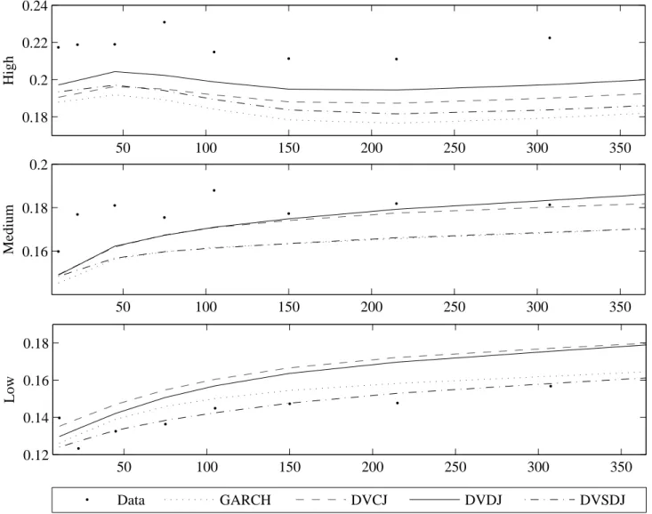
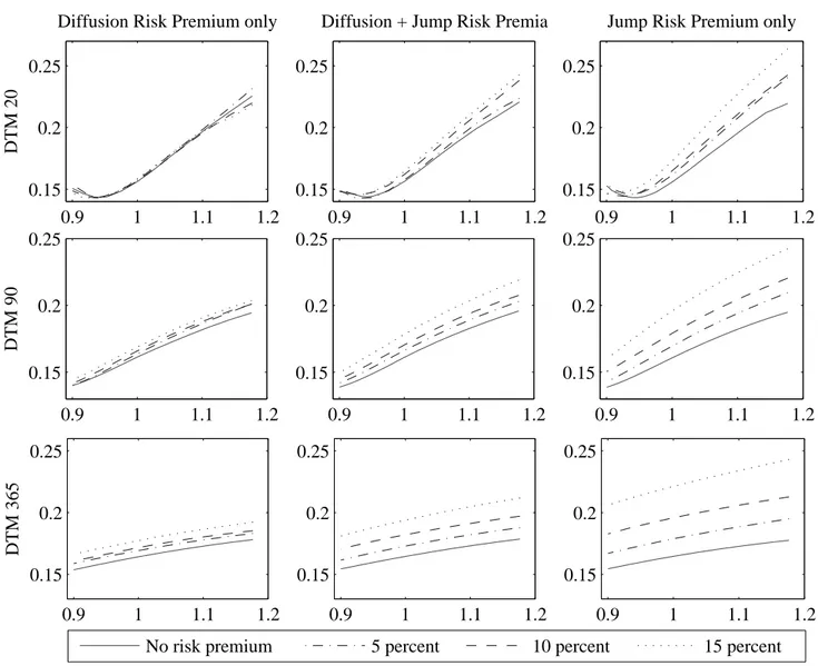
(23) 5.4. The Implied Volatility Bias over Time. Sections 5.2 and 5.3 indicate that the option RMSEs favor the DVDJ model. We now provide more insight into this model’s performance. We first look at the ability of the four models to match the time path of average at-the-money implied volatilities. Figure 6 presents the average weekly at-the-money implied volatility bias (average observed market implied volatility less average model implied volatility) over the 1996-2004 option sample, using the MLE estimates from Tables 2 and 3.6 No model can produce implied volatilities that are sufficiently high to match the data during high-volatility periods. The average biases in Figure 6 are as follows: DVCJ: 0.0274, CVDJ: 0.0373, DVDJ: 0.0256, DVSDJ: 0.0334. These numbers can be compared with the simple GARCH bias of 0.0360. The DVDJ model clearly has the lowest bias, followed by the DVCJ and DVSDJ models. Interestingly, the time paths of implied volatility bias are nearly identical for the DVCJ and DVSDJ models. While the DVDJ model performs the best, overall the models do not differ spectacularly in this dimension.. 5.5. The Implied Volatility Term Structure. The DVDJ performance could also be driven by its ability to better capture the implied volatility term structure. Thus, we now look at the models’ ability to match average atthe-money implied volatility across maturity, for three different volatility periods. Figure 7 presents data and model implied volatility across maturities. In order to investigate the importance of different volatility regimes, we chose three periods each spanning four months. We chose four-month windows because they are small enough to capture different volatility regimes, while still containing sufficient data for robust analysis. The high volatility period (top panel) is from March 1st to June 30th of 2001. The average VIX level in this period is 25.11. The medium volatility period (middle panel) is from March 1st to June 30th of 1997. The average VIX level here is 19.88. Finally, the low volatility period (bottom panel) is from August 1st to November 30th of 2004, with an average VIX level of 16.30. To save space, we do not include the severely misspecified CVDJ model in this figure. Note first that all models underestimate the level of volatility in the high volatility period. The three depicted jump models clearly outperform the GARCH model, which confirms the importance of jumps in the high volatility period. The GARCH model is most biased followed by the DVSDJ and DVCJ models. The DVDJ model performs relatively well in the high volatility period, and produces the least implied volatility bias at all maturities. For the medium volatility period, the DVCJ and DVDJ models perform very well at medium to long maturities, and their performance is quite comparable at all maturities. The DVSDJ model, on the other hand, performs quite poorly with the same level of bias as the GARCH model. For the low volatility period, the DVSDJ model performs relatively well at matching the implied volatility term structure across maturities. On the other hand, the DVCJ and DVDJ models produce volatility levels that are slightly high. The DVCJ model is clearly the most upward biased, and we conjecture that this is due to its constant jump intensity specification, whereas in the DVDJ model, the jump intensity can fall as the level of the variance drops. Overall, the results in Figure 7 support the specification of the DVDJ model. It is the best model at matching the implied volatility levels in the medium and high volatility periods, while producing a slight upward bias in the low volatility period. 6. We consider options to be at-the-money if their strike price lies within 2.5% of the underlying index.. 20.

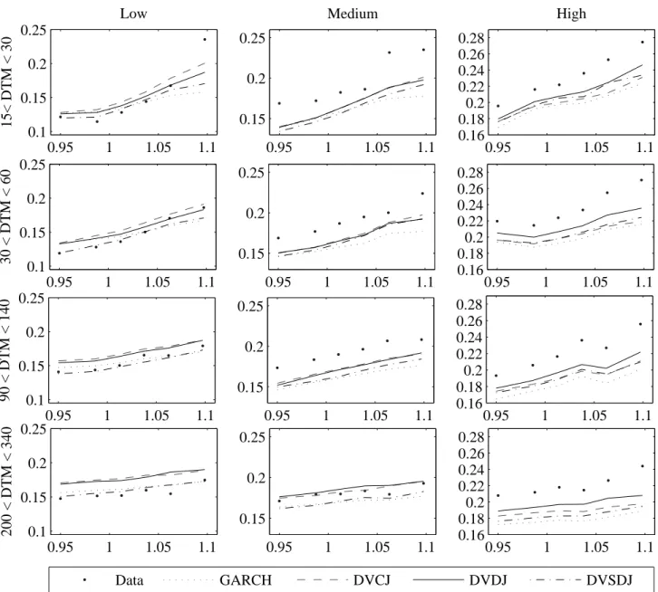
(24) 5.6. The Implied Volatility Smirk. Figure 8 presents the implied volatility smirks implied by the models. For each model, we compute the implied volatility smirk for the three different volatility periods identical to the ones used in Figure 7. In order to reduce the noise in the data, we pool the implied volatilities into moneyness and maturity bins. We plot moneyness smirks for four different maturity ranges (top to bottom): 15 to 30 days, 30 to 60 days, 90 to 140 days, and 200 to 340 days. The left column reports on the low volatility period, while the center and right columns report on the medium and high volatility periods. Again we do not include the misspecified CVDJ model in this figure. In the medium and high volatility periods, we notice that the DVDJ model is the best at matching the implied volatility levels, especially for deep-in-the-money options. The slope of the smirk is fairly flat for all models, and they cannot capture the shape of the smirk implied by short maturity options. Nevertheless, DVDJ performs well compared to GARCH, as it produces a somewhat steeper slope and a much higher level of implied volatility across moneyness. As for the low volatility period, the DVCJ and DVDJ models again produce excessively high implied volatility levels, especially at longer maturities. Nevertheless, the DVDJ model is less biased than the DVCJ, confirming our earlier results. For the DVSDJ model, the performance in the low volatility period is comparable to the GARCH model.. 5.7. Jump Risk Premia and Equity Risk Premia. The option valuation results are based on parameter estimates obtained from physical returns. We now further explore the implications of different risk premia estimates for option pricing performance. We first perform a robustness analysis by investigating alternative assumptions on the equity premium. Subsequently we investigate the different impact of the two risk premium components. We start by relaxing the assumption regarding the model’s implied equity premium. Specifically, we use MLE estimates from Tables 2 and 3 and compute option IVRMSEs for other economically plausible values of the equity premium, while constraining the equity premium to be equal across models. For jump models, we allow both risk premia to jointly contribute to the total equity premium. Table 6 reports option pricing performance based on the IVRMSE metric for different levels of the equity premium. Panel A shows the GARCH IVRMSE. Panels B, C, and D show the IVRMSE ratios for three jump models relative to the GARCH model. In each panel, the columns represents various levels of the equity premium ranging from 0% to 10%. The rows represent various levels of the risk premium associated with the normal component. For example, in Panel C, if the total equity premium is 8% and the risk premium for the normal innovation is 2%, which means that the jump risk premium is 6%, the IVRMSE ratio is 0.86. For this combination of risk premia, the DVDJ model thus improves over the GARCH model by 14%. Note that for the GARCH case, we only have entries on the diagonal since the only source of risk is associated with the normal innovation. First, we investigate the robustness of the option pricing performance of the DVDJ model, this refers to Panel C of Table 6. We see that the DVDJ model performs well compared to the GARCH model at all levels and combinations of the risk premia. It performs particularly well when a large part of the equity risk premium is attributed to jump risk. 21.

(25) Next, we study the option pricing performance of jump models when the equity premium is entirely due to non-jump risk, which corresponds to the diagonal entries. Regardless of the equity premium, option pricing improvements are minimal in the absence of jump risk premia; the DVDJ leads to a 4% improvement, and the DVSDJ actually underperforms the GARCH model. On the other hand, when the equity premium is entirely due to jump risk, the proposed jump models significantly improve on the GARCH model as the total equity premium increases. This corresponds to the bolded cells in the first rows of panels B-D. The strong dependence of option pricing performance on the presence of jump risk premia allows us to conclude that jump risk premia are a necessary element for option pricing in this class of models. The proposed jump models improve option pricing performance through jump risk premia by reconciling the gap between the physical and the risk-neutral measures. To ensure that our finding is not due to a specific choice of loss function, we repeat this analysis using $RMSE instead of IVRMSE (not reported), and identical conclusions obtain. To study the role of jump risk premia in more detail, we further investigate how the option pricing performance of the proposed jump models is affected by the jump risk premia. Figure 9 presents volatility smirks implied by the DVDJ model at three different maturities, for different levels and sources of risk premia. The left column presents results for zero jump risk premia (λy = 0), with total equity premia of zero, five, ten, and fifteen percent. The right column presents results for λz = 0, and the middle column represents the mixed case where each component delivers half the equity risk premium. The conditional jump intensity and conditional variance of the normal component are set equal to their long run mean values. The importance of the jump risk premia is clearly evident. The shape and especially the level of the implied volatility smirks are highly sensitive to the jump risk premium, but not to the risk premium associated with the normal innovation. We have repeated this analysis with the other proposed jump models, and obtain identical conclusions (not reported). For options with 20 days to maturity, increasing the jump risk premia results in steeper slopes. Interestingly, the location of the “hook” also changes as the jump risk premium increases. Our findings are consistent with Bakshi, Kapadia, and Madan (2003), who show that the more negative the risk-neutral skewness (and the higher the risk aversion), the steeper the implied volatility slopes. For longer maturities, we see that high implied volatilities can be generated with small jump risk premia. In the absence of jump risk premia this is not possible. Similar findings can be found in Bakshi, Cao, and Chen (1997) and Bates (2000), who show that the risk-neutral parameters required to fit stochastic volatility models to options prices are unrealistic. Our conclusions regarding the impact of jump risk premia are also in line with BCJ (2007).. 6. Further Analysis of the Models. In this section we further investigate the jump models developed above. First, recall that our models are designed so that the researcher does not need to separately identify the two unobserved shocks zt+1 and yt+1 , neither to estimate the models nor to use them for option pricing. The likelihood is specified in terms of observed underlying returns and the variance and jump dynamics are updated using observed returns rather than using the two unobserved shocks individually. Nevertheless, in order to learn more about the models’ performance we may want to separate the shocks and we do so below using the particle filter. 22.