Etude de la différenciation métal-silicates dans les petits corps du système solaire : une approche pluridisciplinaire

(1)

THÈSE

En vue de l’obtention du

DOCTORAT DE L’UNIVERSITÉ DE TOULOUSE

Délivré par : l’Université Toulouse 3 Paul Sabatier (UT3 Paul Sabatier)

Présentée et soutenue le 26/11/2019 par :

Adrien Néri

Étude de la différenciation métal-silicates dans les petits corps du Système Solaire : une approche pluridisciplinaire

JURY

Renaud Deguen ISTerre-UJF, Grenoble Président du Jury

Valérie Malavergne LGE-UPEM, Paris Rapporteure

Daniel J. Frost BGI, Bayreuth Rapporteur

Brigitte Zanda MNHN-IMPMC, Paris Examinateure

Denis Andrault LMV-UCA, Clermont-Fd Examinateur

Michael J. Toplis IRAP, Toulouse Directeur de thèse

Ghylaine Quitté IRAP, Toulouse Co-Directrice de thèse

École doctorale et spécialité :

SDU2E : Sciences de la Terre et des Planètes Solides Unité de Recherche :

Institut de Recherche en Astrophysique et Planétologie (IRAP - UMR 5277) Directeur(s) de Thèse :

Michael J. Toplis et Ghylaine Quitté Rapporteurs :

(2)

(3)

Remerciements

Ces trois années sont passées très vite, je m’y suis lancé sans trop savoir à quoi m’attendre, mais je me suis pris au jeu. À l’aide de mes quatres directeurs, nous avons réussi à pousser l’aspect multidisciplinaire assez loin, je suis assez fier du résultat final. Tout ce travail n’aurait pas été ce qu’il est maintenant sans le soutien de beaucoup de personnes, que ce soit sur le plan professionel ou amical, je tiens à remercier sincèrement toutes ces personnes.

Tout d’abord, un grand merci à tout mes directeurs, Ghylaine Quitté, Mike Toplis, Jérémy Guignard et Marc Monnereau. Je tiens à souligner l’implication des deux derniers, bien que n’ayant pas de reconnaissance officielle, je les considère comme mes directeurs et les remercie de m’avoir donné de leur temps, ma thèse n’aurait pas été la même sans eux. Je voudrais en profiter pour faire une mention spéciale à Jérémy, qui m’a toujours donné de son temps, même s’il avait d’autres choses à faire. Merci à toi Jérémy.

Merci à Denis Andrault et à Micha Bystricky pour leur implication dans mon comité de suivi de thèse et leurs conseils. Je voudrais dire merci à tout les membres de l’équipe DIP, vous aviez toujours le sourire ça a été très agréable. Je souhaites également remercier toutes les personnes qui m’ont aidé expérimentalement, sur la plateforme de planétologie toulousaine : Jérémy, Frédéric Béjina, Micha et Alain Pagès ; lors des expériences piston-cylindre au LMV à Clermont-Ferrand : Ken Koga et Didier Laporte ; lors des expériences en presse Paris-Edimbourg lors de notre session à SOLEIL : Denis, Jean-Philippe Perrillat, Micha, Ghylaine, Marc, Jérémy, Andrew King et Nicolas Guignot. Merci à tout ceux m’ont aidé à réaliser les analyses sur mes échantillons, surtout à l’équipe du centre de microcaractérisation Raimond Castaing : Stéphane Leblond du Plouy pour le MEB, Sophie Gouy et Philippe de Parseval pour la microsonde électronique, ainsi que Claudie Josse et Arnaud Proietti pour l’EBSD ; mais aussi à Christophe Tenailleau et Benjamin Duployer du CIRIMAT pour les analyses de microtomographie 3D.

Je tiens à remercier tout les membres d’UniverSCiel avec lesquels j’ai pu animer le festival Astro-Jeunes à Fleurance, ou d’autres interventions, ça aura été un réel plaisir de travailler avec vous. Merci également à tout les thésards de l’IRAP avec qui j’ai pu passer de très bons moments. Un grand merci à l’équipe des "Bras Cassés" : Mathilde, Louise, Pauline, Edoardo et Geoffroy pour toutes les escape game que nous avons fait à Toulouse. Merci aux copains Lyonnais, que ce soit du Parc : Jean et Valentin, ou de l’ENSL : Alexandre, Antonin, Thomas et Valentin. Je voudrais finir ce paragraphe par dire merci à mes amis proches arlésiens : Jérémy et Vincent, mes bros, "The Wolf Pack", avec qui je suis resté en contact pendant toutes ces années malgré la distance.

Pour finir, je voudrais remercier ma famille, qui m’a toujours soutenu dans ce que je voulais faire. Merci tout particulièrement à mes parents et à mon frère. Merci à toi Mathilde ma chérie d’avoir partagé ces années avec moi, merci pour tout ce que tu m’apportes et merci de me rendre meilleur.

Adrien i

(4)

(5)

List of Figures

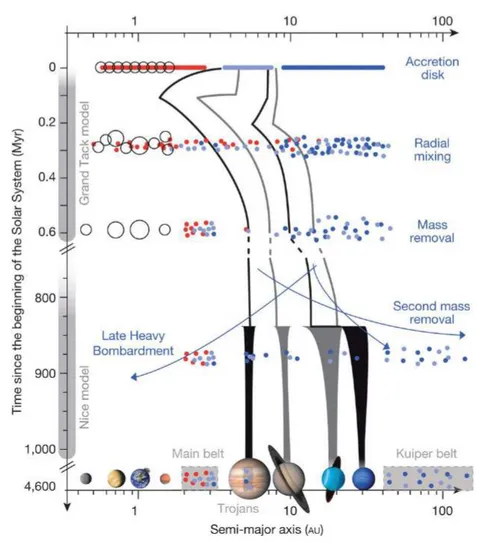
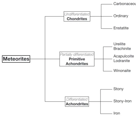
1.1 Cartoon illustrating planetary migrations and the effect on the asteroid belt (Demeo and Carry, 2014). The orbit of the gas giants are represented in black and gray lines. Planetesimals are represented as dots which color depends on their accretion region: red for the disk, light blue for the gas giants region and dark blue the region beyond the gas giants. There are two main events of planetary migration: the Grand Tack model that occurred early in the Solar System history and the Nice model that took place much later, around 700 Myr. During the Grand Tack, Jupiter migrated inward due to gas-drag, until Saturn catches it back and enters into a resonant motion, driving both giants back to their original region. Uranus and are also pushed back. During this inward then outward migration, planetesimals that accreted near the Sun and in the gas giants region are mixed together. Terrestrial planets are formed from a truncated disk, except for Mars that formed from embryos that were scattered out of the disk. After a long quiescent period of ¥ 700 Myr, Jupiter and Saturn entered in a new resonant motion, driving their orbit and that of Uranus and Neptune into chaotic motions with close encounters between the giants (Nice model). This destabilized the outer planetesimal disk and the asteroid belt, scattering objects all over the Solar System, shaping the asteroid and the Kuiper belts and inducing the Late Heavy Bombardment. This event is the last major event that reshaped the Solar System into what is observed today. . . 12 1.2 Simplified meteorites classification with emphasis on the differentiation degree

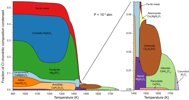
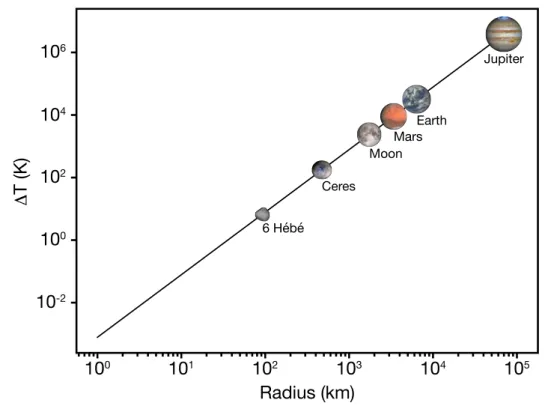
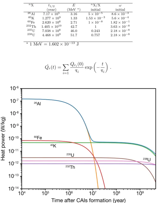
of the different objects. . . 14 1.3 Condensation sequence of a CI chondrite material from Davis and Richter (2013). 15 1.4 Temperature increase (in K) due to the accretion as a function of the radius of

the newly formed body (in km). For this calculation, the mean calorific capacity is taken as 750 J.kg≠1_.K≠1 _{and the mean density as 3500 kg.m}≠3_{. . . .} ₂₂ 1.5 Heat power per mass unit generated from the decay of radionuclides in a CI

chondritic material as a function of time after the formation of CAIs. The blue curve represents the total power. . . 23 1.6 Core temperature as a function of time since CAIs formation for (a) different

radii and an accretion date of 1 Myr after CAIS and (b) different accretion time for a body with a radius of 100 km. Red curves represent the heat power per volume unit due to26_{Al decay. (Marc Monnereau, personal communication) 24}

(8)

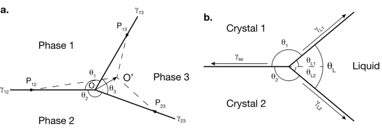
1.7 Sketch showing the 2D organisation of a triple junction in a three-phase system (a) and in a two-phase system (b), between two solid crystals and a liquid. ◊ are dihedral angles and “ are interfacial energies. “SS stands for the solid-solid

interfacial energy and ◊L for the liquid dihedral angle. . . 26

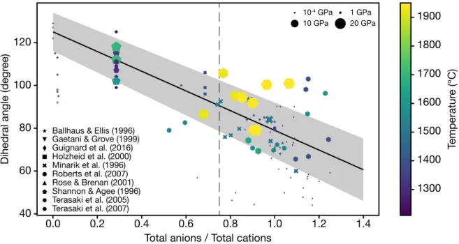
1.8 Interconnection threshold as a function of dihedral angle for tetrakaidecahedra or irregular shaped crystals. The analytical solution of Wray (1976) is repre-sented in red. The trapping threshold corresponds to the green curve. Dashed lines represent extrapolation of the numerical simulations to higher dihedral angles. This plot is adapted from Laporte and Provost (2000); Ghanbarzadeh et al. (2017). . . 29 1.9 Dihedral angle as a function of the total anions to total cations ratio. This data

compilation has been updated since Holzheid et al. (2000). Data were taken from Ballhaus and Ellis (1996); Gaetani and Grove (1999); Guignard et al. (2016); Holzheid et al. (2000); Minarik et al. (1996); Roberts et al. (2007); Rose and Brenan (2001); Shannon and Agee (1996); Terasaki et al. (2005, 2007). The thin dashed line represent the Fe-FeS eutectic composition at 1 bar. With increasing pressure, the eutectic is likely to be depleted in sulfur, shifting this dashed line toward lower anions to cations ratios, e.g. 0.56 at 10 GPa (Buono and Walker, 2011). . . 31 1.10 Core pressure (green curve) and surface gravity (red curve) as a function of the

planetesimal radius. Density is taken to be 3500 kg.m≠3_{. . . .} ₃₃ 1.11 Darcy time as a function of compaction time for different fixed draining times

(gray lines). The dashed line, which equation is „0R/Lc= 4, separates regimes

controlled by the compaction of the matrix (white) from regimes controlled by the Darcy flow time scale (grey region). The green dot indicates the draining time for a body with a radius of 100 km, while the blue one that of a planetes-imal with a radius of 20 km. The dashed blue arrow shows the trend for bodies with radii lower than 20 km. . . 36 1.12 Iron-sulfur phase diagram at 1 bar. . . 41 1.13 Critical height for a network to sink as a function of the silicate matrix crystal

radius. Left panel is drawn for a crystal fraction of 0.65 and right panel for a crystal fraction of 0.75. Dashed line represents a eutectic composition of the iron-sulfide network while full line represents a pure iron composition. Blue is for a planetesimal with a radius of 100 km and orange for a radius of 300 km. Values of interfacial energies were taken from Holzheid et al. (2000) and Néri et al. (2019). . . 42

(9)

List of Figures vii

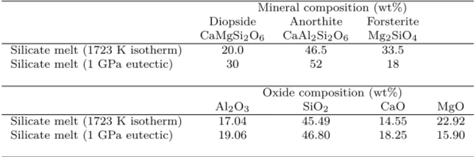
2.1 Anorthite - Diopside - Forsterite ternary diagram at 1 bar (adapted from Pres-nall et al., 1978). The white region corresponds to the domain of composition in which the silicate melt is in equilibrium with forsterite, black lines correspond to limits between each equilibrium region and dashed lines correspond to the isotherm curves. Temperatures are written in degrees Celsius. The red curve corresponds to the 1723 K isotherm and the blue dot to the aimed silicate melt composition. . . 47 2.2 Anorthite - Diopside - Forsterite ternary diagram at 1 GPa (adapter from

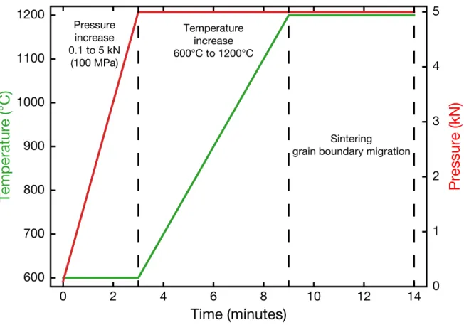
Pres-nall et al., 1978). The white region corresponds to the domain of composition in which the silicate melt is in equilibrium with forsterite, black lines corre-spond to limits between each equilibrium region and dashed lines correcorre-spond to the isotherm curves. Temperatures are written in degrees Celsius. The blue dot corresponds to the aimed composition which is the same that at 1 bar. The green line represents the evolution path of a glass of the 1 GPa eutectic composition that reacts with forsterite upon temperature increase. . . 49 2.3 Sintering pressure - temperature path. The green curve shows the evolution of

temperature with time and the red curve the evolution of pressure with time. Pressure is first increased up to 100 MPa, then temperature rises to 1473 K, favoring sintering and grain boundary migration without melting of the silicate glass. . . 50 2.4 Atmosphere controlled high temperature furnace setups. (a.) Scheme of the

alumina rod with fours holes that allow suspending the samples and temper-ature measurement with a type S thermocouple. (b.) Sketch of the wire loop technique. (c.) Sketch of a piece of a sintered sample put in a nickel basket and on an alumina disk. This last setup is only valid for temperatures lower than that of nickel melting, i.e. lower than 1728 K. . . 52 2.5 (a.) Evolution of the oxygen fugacity as a function of temperature along the

NNO and IW buffers, and the experimental conditions, i.e. three log units below the NNO buffer. (b.) Evolution of the gas fluxes (CO2 and CO) along the different trends (IW, NNO and NNO - 3) as a function of temperature. Thin black dashed lines illustrate the experimental conditions: 1713 K and

NNO = ≠3 . . . 55 2.6 Piston-Cylinder experimental setup. . . 57 2.7 Paris-Edinburgh press experimental assembly. . . 59 2.8 Composition of atmosphere controlled 1-bar high temperature furnace

experi-ments. Oxygen fugacity is set to 10≠8.46 _{and temperature to 1713 K for} experi-ments with solid nickel (red dots) or 1743 K for experiexperi-ments with molten nickel (blue dots). Experiment duration is typically 24h. Orange dots correspond to a time-serie experiment with solid nickel. Green dots represent a time-serie experiment of samples that experienced 24 h at 1713 K and then different duration at 1743 K. . . 60

(10)

2.9 Composition of piston-cylinder experiments. Pressure is set to 1 GPa and tem-perature to 1723 K for experiments with solid nickel and to 1773 K for ex-periments with molten nickel. A two-step experiment that underwent a first equilibration for 5 h at 1723 K and then 3 h at 1773 K was also prepared for comparison with the time-serie experiment in atmospheric furnace. . . 61

2.10 Composition of Paris-Edinburgh press experiments. Pressure is set to 1 GPa and temperature varied up to ¥ 2123 K.Experiments were conducted either with pure nickel (black dots), no metal (green dot), nickel sulfide with a eutectic composition (gray dots) or an intermediate composition giving Ni0.9S0.1 in stoichiometry (white dots). . . 62

2.11 Schemes showing the different incident electron - matter interactions used for the analytical techniques. (a.) Generation of backscattered electrons. (b.) Gen-eration of secondary electrons. (c.) GenGen-eration of X-rays. . . 64

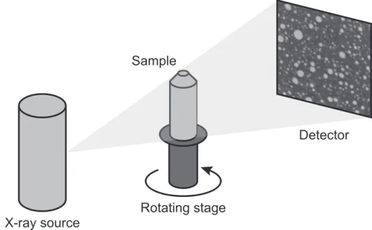
2.12 Scheme showing the principle of 3D X-ray microtomography analysis. . . 66

3.1 SEM images representative of different samples. White: nickel; dark gray: forsterite and light gray: silicate melt. (a.) 47.5:47.5:5 sample at ◊1, 000 (94 nm per pixel), (b.) 62.5:32.5:5 samples at ◊1, 000 (94 nm per pixel), (c.) 20:75:5 sam-ple at ◊1, 000 (94 nm per pixel), (d.) 75:20:5 samsam-ple at ◊1, 000 (94 nm per pixel), (e.) 20:75:5 sample ◊3, 000 (30 nm per pixel), (f.) 75:20:5 sample at ◊3, 000 (30 nm per pixel), (g.) 20:75:5 sample at ◊10, 000 (9.4 nm per pixel), (h.) 75:20:5 sample at ◊10, 000 (9.4 nm per pixel). Images on (g.) and (h.) highlight the hook shape of the silicate melt toward the apex of triple junc-tions. This kind of structure is typically of 100 nm at half-height of the hook, requiring a resolution threshold of 30 nm per pixel to have a proper imaging. 75

(11)

List of Figures ix

3.2 Measured median dihedral angle as a function of pixel size (in nm) for (a.) silicate melt, (b.) forsterite, (c.) nickel and merged dihedral angles distributions at different pixel sizes: (d.) 376nm per pixel, (e.) 94nm per pixel and (f.) 30 and 9.4nm per pixel. Circle color symbols on (a.), (b.), (c.) correspond to different samples, black circle represents the median value of all datasets merged at a given magnification and gray lines are guides for the eyes. These three diagrams show that the dihedral angle reaches steady value at a pixel size of 30 nm per pixel, corresponding to the resolution at which the fine microstructure is entirely imaged. Scatter between different samples at lower resolution is due to measurement artifacts, as this small-scale geometry is not entirely imaged. Step curves on (d.), (e.) and (f.) correspond to the dihedral angle distribution, curly curves correspond to Gaussian fits, single Gaussian function for (d.) and (e.) and triple Gaussian function for(f.); black dotted lines represent the median value of the distributions. The agreement between data and triple Gaussian fit is shown in (g.) for the silicate melt distribution and in (h.) for the olivine distribution. Orange, green and blue dotted vertical lines correspond to median values of each subset of dihedral angle. Increasing the resolution makes the distribution more asymmetric, meaning that different populations of dihedral angle exist, representative of the forsterite crystalline anisotropy at microscale. 78 3.3 Schematic vie of a triple junction between the silicate melt, a forstertite crystal

and a nickel grain. Dihedral angles ◊1, ◊2 and ◊3 are related to interfacial ener-gies “12, “13and “23 when textural equilibrium is achieved, following equation 3.2 . . . 80 3.4 (a.) Ternary diagram showing the inner triangle of possible space given the

conditions ◊ > 0° and ◊ < 180°. (b.) Reduced ternary diagram showing the different energetic regimes delimited by equation 3.3. Full lines separate these regimes and represent equality between two interfacial energies. Sketches ex-plaining the geometry in remarkable points of the ternary diagram are repre-sented in (c.) and (d.). Two end-member cases are considered: (c.) metal is the minor phase, (d.) silicate melt is the minor phase. If one angle is equal to 180°, the phase either forms a sphere or a film. When the dihedral angle is equal to 0°, the phase is highly wetting, its contact is punctual or inexistant, and this phase prevents the two others from being in contact with each other. . . 82 3.5 Ternary diagram of the dihedral angles with the different energetic regimes.

Pruple symbols represent data from this study. Pentagon symbols stand for the different populations of dihedral angle taking into account forsterite crystalline anisotropy (merged data at resolutions of 30 and 9.4 nm per pixel). Gray sym-bols correspond to the data from Holzheid et al. (2000). Error bars are smaller than symbols. Sketches show the geometry of the three phases according to their dihedral angles. Color code is the same as in Figure 3.3, except for sulfide, in red. Data with pure metal fall in the “Melt≠Fo < “_Melt≠Ni< “_Fo≠Nidomain, even when crystalline anisotropy is taken into account (shaded pentagons), which is clearly different from a system with sulfide: “Melt≠Sulfide< “_Melt≠Ol< “_Ol≠Sulfide. 83

(12)

3.6 Evolution of the metal volume fraction of a silicate-metal mixture as a function of temperature. Silicate melt is assumed to be continuously extracted so that the metal fraction increases with the melting degree of silicate. The metallic melt is completely drained when its percolation threshold is reached, except a trapped fraction set to 1 vol%. The percolation threshold is a function of the sulfur content. (a.) Different interconnection threshold evolutions as a function of sulfur content of the sulfide melt. (b.) Percolation threshold functions as a function of temperature. Full lines are for simulations that experienced sulfide melt extraction once all the iron is molten, while dashed lines represent the case where the extraction occurred when a solid iron residue was present. (c.) Evolution of the metal volume fraction (solid iron and sulfide melt) as the sil-icate is extracted through fractionated melting. (d.) Evolution of the sulfide melt volume fraction as a function of temperature. In (c.) and (d.) the black line represents the volume of silicate melt extracted as a function of temper-ature, the shaded area indicating the residual silicate. The different kinks in the silicate melting curves represent the disappearance of mineral species, ar-rows pointing them out. Color lines draw the volume fraction of the metallic subsystem in (c.) and of the sulfide melt in (d.) for the different percolation threshold functions depicted in (a.) and (b.). . . 86

3.7 Evolution of the sulfur content of metal plotted on the phase diagram of the Fe-FeS system. Color dots represent the composition of the extracted melt, fol-lowing the color code for the different threshold functions of Figure 6a. Color bars represent the composition of different primitive achondrites, sulfur en-riched ones in pink (Acapulco Guignard and Toplis (2015); Zipfel et al. (1995) and TIL99002 Patzer et al. (2004)) and S-depleted ones in yellow (Acapulco Palme et al. (1981), Lodran Bild and Wasson (1976); Guignard and Toplis (2015) and NWA 725 Patzer et al. (2004)). The discrepancy in the sulfur con-tent of the different primitive achondrites can be accounted for given that the evolution of the interconnection threshold is close to threshold functions (d) or (e), allowing the fractionation of sulfur within the planetesimal. . . 87

4.1 Textures comparison of nickel phase (5 vol% in all samples) between stirred by gas bubbles samples (1-bar furnace, AF) and immobile samples (piston cylinder, PC) for different proportions of silicate melt in the system and after 24 hours (AF) and 5 hours (PC) of experiments at 10-15 K below the melting point of nickel. (a-c) show images of the 3D X-ray microtomograms. In gray is represented all the nickel of the sample. The three biggest blobs of nickel are represented in red, orange and yellow in each sample. (d-f) represent the volume to surface ratio (V/S) as a function of blob volume, with data points for AF experiments in red and data points for PC experiments in black. Normalized distributions (V/Vmean), in volume or in number are represented in (g-i) and (j-l), respectively. Here also, AF data are plotted in red and PC data in black. 100

(13)

List of Figures xi

4.2 Results of the EBSD data acquired on the 20:75:5 (Fo:Melt:Ni vol%) AF time-series experiments at 1713 K (with solid nickel). The first column correspond to a run duration of 0.5 hours, the second column to a run duration of 2 hours, the third column to a run duration of 6 hours and the last column to a run duration of 24 hours. (a-d) Phase identification of the analyzed surfaces, with nickel grains in red and forsterite crystals in green. Silicate melt and air bubbles are represented in black. (e-h) Local misorientation maps of the phases, with low misorientation angles in blue and high misorientation angles in red. The color scale is normalized to the same maximum value of 5° for both phases and for the different maps. Grain boundaries appear in thick black lines while sub-grain boundaries in thin black lines. (i-l) Distributions showing the evolution of aspect ratios of forsterite and nickel with time. Forsterite is represented in green and nickel in red. Dashed lines correspond to the mean aspect ratio of a phase. . . 104 4.3 Time-series textural evolution of nickel phase across the melting temperature of

nickel in sample containing 75 vol% of silicate melt and stirred by gas bubbles (AF experiments). (a, e and i) are the same diagrams that in Figure 4.1. (a-d) show images of the 3D X-ray microtomograms and the V/S ratio as a function of blob volume. In gray is represented all the nickel of the sample. The three biggest blobs of nickel are represented in red, orange and yellow in each sample. Normalized distributions (V/Vmean), in volume or in number are represented in (e-h) and (i-l), respectively. . . 105 4.4 Textural evolution of nickel phase with varying forsterite to forsterite plus

silicate melt ratios (noted as Fo / (Fo + Melt); 90% in red, 80% in blue and 70% in green) and varying nickel content (10 vol% in the first column, 15 vol% in the second one and 20 vol% in the third one). The three rows show similar representations to those used in Figure 4.3. (a-c) The largest blob of each experiment is represented in color corresponding to the Fo / (Fo + Melt) ratio, along with the V/S ratios of the blobs in the different samples. Normalized distributions (V/Vmean), in volume or in number are represented in (d-f) and (g-i), respectively. . . 107 4.5 Textural evolution of nickel phase in the Paris-Edinburgh press experiments

conducted on beamline PSICHE (SOLEIL Synchrotron) for three different mix-tures (in Fo:Melt:Ni vol%): 65:25:10 (in red), 70:5:25 (in green) and 65:5:30 (in blue). Results here are plotted as a function of temperature, which corresponds also to a different silicate melt content due to progressive melting. For simplic-ity, the nickel volume fraction (a) and the SNSVR (b) of the largest blob are plotted as a function of temperature. Numbers represent images of the 3D to-mograms in different conditions and for the different samples. For clarity of the figure, only the three largest are represented in red, orange and yellow, from largest to third largest. . . 108

(14)

5.1 Temperature (green curve) and viscosity as a function of crystal fraction for different rheological thresholds (black, red and pink curves). The green curve is the result of an equilibrium melting simulation of a chondritic material (H chondrite) using the Rhyolite MELTS thermodynamical simulator (Asimow and Ghiorso, 1998; Ghiorso and Gualda, 2015; Ghiorso and Sack, 1995; Gualda et al., 2012). The different kinks in the curve correspond to the complete melt-ing of a mineral phase. The viscosity - crystal fraction relation is drawn from the Einstein-Roscoe equation (eq. 5.1 Roscoe, 1952). The temperature and viscosity y-axis are not correlated. . . 118 5.2 Sketch showing the thermal structure of a planetesimal that melted enough

to have a deep magma ocean (crystal fraction „ < maximum packing fraction „m). The grey shaded layer corresponds to the conductive lid, Tsurf is the

surface temperature, T („m) is the temperature at which the crystal fraction

corresponds to „m, Tm is the temperature of the magma ocean, ” is the

bound-ary layer thickness and ◊ is the temperature difference within this boundbound-ary layer (◊ = Tm≠ T („m)). . . 119

5.3 Viscosity as a function of temperature following Roscoes’s law (equation 5.1, dashed curves) and fluid temperature as a function of the Rayleigh number, (a.) for different maximum packing fraction at a fixed radius of 100 km and (b.) for different radii at fixed „m. The gray thin lines show the equilibrium

parameters for the different cases studied here. These calculations are for an accretion date of 1 Myr after CAIs. . . 121 5.4 Metal minimum grain size to escape convective motions as a function of

viscos-ity for (a.) different „m at fixed radius and (b.) for different radii at fixed „m.

Vertical and horizontal lines show the equilibrium parameters for the different cases studied here. These calculations are for an accretion date of 1 Myr after CAIs. . . 123 5.5 Grain growth laws for olivine (green curve, Faul and Scott, 2006) and nickel

(red curve, Guignard et al., in prep.) as a function of time. Temperatures are taken from the equilibrium configuration of magma oceans. Full lines are for the equilibrium temperature with a maximum packing fraction of 0.6; while shaded areas are for equilibrium temperatures with „m ranging from 0.5 to 0.7. 125

5.6 Metal volume fraction as a function of silicate melting degree. The metal volume fraction does not correspond to the absolute content as it represents the fraction after removal of a given silicate melt fraction, corresponding to that of the x-axis. The color map shows the evolution of the fayalite content of olivine, with the gray areas showing the value corresponding to that of main group pallasites (12 mol%, Boesenberg et al., 2012). The thin black curves show the complete melting of the different silicate phases: Cpx for clinopyroxene, Flp for feldspar and Opx for orthopyroxene. Gray shaded areas show the melt fractions corresponding to the equilibrium magma ocean with the effect of accretion date and size as lateral variations; the horizontal area shows the corresponding metal fraction after silicate melt extraction. . . 128

(15)

List of Figures xiii

5.7 Sketch showing the final structure of a planetesimal that underwent a magma ocean stage. . . 129 6.1 (a.) Fe-Ni-Cr-P-S-Cr EDS map, (b.) Si-Al-Na-Mg-Ca EDS map and (c.) local

misorientation map of Dhofar 1222. The local misoriention plots only the phases with the best EBSD signal, i.e. olivine, orthopyroxene and kamacite-taenite. . 136 6.2 (a.) Fe-Ni-Cr-P-S-Cr EDS map, (b.) Si-Al-Na-Mg-Ca EDS map and (c.) local

misorientation map of NWA 725. The local misoriention plots only the phases with the best EBSD signal, i.e. olivine, orthopyroxene and kamacite-taenite. . 138 6.3 (a.) Fe-Ni-Cr-P-S-Cr EDS map, (b.) Si-Al-Na-Mg-Ca EDS map and (c.) local

misorientation map of Acapulco. The local misoriention plots only the phases with the best EBSD signal, i.e. olivine, orthopyroxene and kamacite-taenite. . 139 6.4 (a.) Fe-Ni-Cr-P-S-Cr EDS map, (b.) Si-Al-Na-Mg-Ca EDS map and (c.) local

misorientation map of A 881902. The local misoriention plots only the phases with the best EBSD signal, i.e. olivine, orthopyroxene and kamacite-taenite. . 140 6.5 (a.) Fe-Ni-Cr-P-S-Cr EDS map, (b.) Si-Al-Na-Mg-Ca EDS map and (c.) local

misorientation map of Dhofar 125. The local misoriention plots only the phases with the best EBSD signal, i.e. olivine, orthopyroxene and kamacite-taenite. . 141 6.6 (a.) Fe-Ni-Cr-P-S-Cr EDS map, (b.) Si-Al-Na-Mg-Ca EDS map and (c.) local

misorientation map of MET 01198. The local misoriention plots only the phases with the best EBSD signal, i.e. olivine, orthopyroxene and kamacite-taenite. . 142 6.7 (a.) Fe-Ni-Cr-P-S-Cr EDS map, (b.) Si-Al-Na-Mg-Ca EDS map and (c.) local

misorientation map of Monument Draw. The local misoriention plots only the phases with the best EBSD signal, i.e. olivine, orthopyroxene and kamacite-taenite. . . 143 6.8 (a.) Fe-Ni-Cr-P-S-Cr EDS map, (b.) Si-Al-Na-Mg-Ca EDS map and (c.) local

misorientation map of Lodran. The local misoriention plots only the phases with the best EBSD signal, i.e. olivine, orthopyroxene and kamacite-taenite. . 145 6.9 (a.) Fe-Ni-Cr-P-S-Cr EDS map, (b.) Si-Al-Na-Mg-Ca EDS map and (c.) local

misorientation map of GRA 95209. The local misoriention plots only the phases with the best EBSD signal, i.e. olivine, orthopyroxene and kamacite-taenite. . 146 6.10 Lattice preferred orientation of troilite grains in Lodran. Lower hemisphere

and equa-area projection in the sample coordinate system. The color code correspond to the density of Multiples of Uniform Distribution (MUD). N is the number of grains measured. To give equal weights to the different grain, each grain was considered as a single point. . . 149 6.11 Silicate grain size distributions normalized to the mean grain size. Heights of

(16)

6.12 Kamacite-taenite grain size distributions normalized to the mean grain size. Heights of the distributions are normalized to the maximum height. . . 152 6.13 FeO and MgO composition profile within an olivine of Lodran. Compositions

are reported in oxide wt%. . . 153 6.14 Wollastonite (Ca2Si2O6) - Ferrosilite (Fe2Si2O6 - Enstatite (Mg2Si2O6) ternary

diagram with the mean compositions of ortho- and clinopyroxenes reported. Er-ror bars represent two standard deviation with respect to each pure endmember.154 6.15 Orthose (KAlSi3O8) - Anorthite (CaAl2Si2O8) - Albite (NaAlSi3O8) ternary

diagram with the mean compositions of feldspars reported. Error bars represent two standard deviation with respect to each pure endmember. Ab stands for Albite, Olg for Oligoclase and An for Anorthite. . . 159 6.16 Oxygen fugacity (expressed as deviation from the IW buffer in log units) as

a function of the closure temperature calculated. Squares correspond to the pyroxene equilibrium while circles correspond to the olivine equilibrium. . . . 164 6.17 Plot showing the time necessary to reach the measured grain sizes of olivine as a

function of that required for kamacite-taenite grains for the different sections. Circles indicate grain growth laws of Guignard et al. (2012, 2016) in a dry system. Squares indicate grain growth laws of Guignard (2011) in a system bearing silicate melt. The colors correspond to the different sections of this survey. The dashed grey line has a slope of one. If metal and silicate grew in similar conditions, which is likely to be the case, natural samples should fall on this line. Deviation to this line seem to indicate Zener pinning growth mechanisms. . . 168 6.18 Timescale of melt migration as a function of the a/Ôµf and R/Ôµm ratios,

which correspond to the Darcy and the compaction timescales respectively. Acapculoite-lodranite parent body is thought to have a radius ranging from 60 (Golabek et al., 2014) to 260 km (Neumann et al., 2018). The different grain sizes determined in the acapulcoite-lodranite-winonaite samples of this study are represented. 50 µ corresponds to the mean winonaites and the A 881902 and Monument Draw acapulcoites. 100 µm corresponds to the mean grain size of most acapulcoites and GRA 95209. 200 µm corresponds to the mean grain size of Lodran or to that of acapulcoites reported in literature (e.g. Keil and McCoy, 2018, and references therein). Finally, 500 µm corresponds to the mean grain size of lodranites as reported by Keil and McCoy (2018, and references therein). Viscosity of the silicate melt is taken to be 10 Pa.s (Dingwell et al., 2004), while that of the silicate matrix is 1018_{Pa.s (Hirth and Kohlstedt, 2003).} Viscosity of iron-sulfur melts is taken to 10≠2 _{Pa.s (Dobson et al., 2000). . . . 170}

(17)

List of Figures xv

6.19 Scheme showing the evolution of a parent body to form winonaites, acapul-coites and lodranites, based on the textural arguments described in this Chap-ter. Dashed lines correspond to boundaries between the different categories of primitive achondrites. The red line indicates the Fe-FeS eutectic; due to the low viscosity of metallic melts, they are expected to migrate over short timescales provided that they form an interconnected network. The green line indicates the silicate eutectic; efficient segregation of the silicate melts is not possible until large grain sizes are reached (¥ 200 µm). Red and green arrows indicate the absolute proportions and the migration of sulfur-rich and silicate melts, respectively. (a.) Scenario giving a deep origin of winonaites and pos-sibly sulfur-enriched acapulcoites. For the sake of simplicity, both categories were represented on the same parent body, but they are not due to their dif-ferent oxygen isotopic composition (Greenwood et al., 2012, 2017) and their different oxygen fugacities (Table 6.9). (b.) Scenario giving a shallow origin of acapulcoites, similarly to the models of Golabek et al. (2014) and Neumann et al. (2018). The grey shaded area indicates part of the body which may be more evolved than lodranites, its thickness is likely to be large following the model of Neumann et al. (2018).Schemes are not to scale. . . 171 6.20 (a.) Olivine Mg# as a function of temperature and (b.) relative olivine volume

fraction (olivine / (olivine + orthopyroxene) ratio) as a function of temper-ature, both for different oxygen fugacity conditions: FMQ = ≠5 ( IW = ≠1.5) in dashed line, FMQ = ≠6 ( IW = ≠2.) in full line and FMQ = ≠7 ( IW = ≠3.5) in dashed-dotted line. Color dots correspond to the acapulcoites and color squares to the lodranites. Vertical errorbars for the Mg# correspond to the 2SD from Table 6.5 and horizontal ones are estimated to be ±100 °C. . 174 A.1 From equations 3.2 and 3.3 in the main text (chapter 3), the value of each

interfacial energy ratio can be calculated for each triplet of dihedral angles. In each diagram, the straight-line represents an interfacial energy ratio equal to 1, other curved lines representing the isovalues for different ratios. Most of the dihedral angle values map variations of interfacial energy ratios over two orders of magnitude, from 0.1 to 10. Close to the iso-line of 1, the ratio of interfacial energies barely varies. However approaching each apex and edge of the ternary diagram (with the exception of the edge orthogonal to the 1:1 line), curves of constant energy ratio are increasingly closely spaced, requiring very precise measurements of dihedral angles to determine interfacial energy ratios accurately. . . 187 A.2 Evolution of the percolation threshold function (dashed line) and of the

asso-ciated sulfide melt content (full line) as a function of temperature. Figures (a), (b), (c), (d) and (e) correspond to different threshold functions as defined on figure (f). Each time the sulfide melt curve crosses tha of the interconnection threshold, i.e. when its content is greater than the interconnection threshold, the sulfide is extracted and only a trapped fraction - set to 1 vol.% (see chapter 3 for more details) - is left. . . 188

(18)

(19)

List of Tables

1.1 Physical parameters of radioisotopes that contribute to heating the interior of planetesimals. nX is the isotope n of element X and Ê is its mass fraction in

CI type chondrites. . . 23 2.1 Mineral and oxide composition of the silicate melt in equilibrium with forsterite

in weight percent. These values correspond to the blue dot in figure 2.1. . . . 48 2.2 H chondrite composition (in wt%) used for the MELTS thermodynamic

sim-ulations (from Wasson and Kallemeyn, 1988); the FeO content is calculated from the FeO/(FeO + MgO) ratio. . . 67 3.1 Composition in wt% of the starting materials and composition of the different

phases after experiments. Error bars, expressed as 2‡ standard deviation, were estimated based on repeated measurements of at least 30 points for each phase. Phase composition of samples are expressed in volume proportions following Fo:Melt:Ni. . . 74 3.2 Median dihedral angles (in °) at the triple junctions for different magnifications

and all samples. The merged sections correspond to all datasets put together. In each column, the value of the dihedral angle is reported with its 2SE (2SE =

2SD Ô

N≠1 where SD is the standard deviation and N the number of measurements) uncertainty. . . 77 3.3 Dihedral angles of the different phases when crystalline anisotropy is considered

and corresponding interfacial energy ratios.ú _{Correspond to values calculated} from dihedral angle data. Uncertainties are 2SE calculated using the derivative method. . . 79 4.1 Starting phase proportions and 3D X-Ray microtomography resolutions of the

different experiments. Proportions are expressed as forsterite (Fo) : silicate melt (Melt) : nickel (Ni) in volume percent. AF is for the 1-bar atmosphere controlled high temperature furnace experiments, PC is for the piston-cylinder experiments and PE for the Paris-Edinburgh press experiments. N.D. are for experiments which were not analyzed with 3D X-Ray microtomography. . . . 96 6.1 List of Primitive Achondrite samples used in this study. . . 135 6.2 Summary of the petrological observation on the different sections. Mineral

ab-breviations stand for: Cpx = clinopyroxenes, Flp = Feldspar, Ol = Olivine and Opx = orthopyroxene. Phase loss or gain are referred to as "n.d." if the depletion or enrichment was not observed qualitatively. . . 147

(20)

6.3 Modal compositions of the samples (in vol%). . . 147 6.4 Mean grain sizes of the different sections. The mean sizes here do not

corre-spond to the arithmetical means, but to the equivalent diameter of the mean surface area of the grains. Two standard errors (2SD

ÔN, with SD the standard deviation) are displayed in parentheses. N gives the number of grains detected. 150 6.5 Olivine and chromite compositions measured in this study (in wt%). Two

stan-dard deviations are displayed in parentheses. N gives the number of measure-ments. . . 155 6.6 Orthopyroxene and Clinopyroxene compositions measured in this study (in

wt%). 2-standard deviations are displayed in parentheses. N gives the number of measurements. . . 156 6.7 Feldspar, troilite and kamacite-taenite (Fe-Ni alloy) compositions measured in

this study (in wt%). 2-standard deviations are displayed in parentheses. N gives the number of measurements. . . 157 6.8 Bulk composition (in wt.%) of the sections calculated from the modal and

phases compositions. . . 158 6.9 Closure temperature and oxygen fugacity (log(fO2)) calculated for different

thermodynamic equilibria. Values calculated for each olivine-chromite (Ol-Chr) mineral pair in Lodran are displayed. IW corresponds to the distance to the Iron-Wustite buffer, in log units. QIFs and QIFa stand for Quartz-Iron-Ferrosilite (equilibrium 6.4) and Quartz-Iron-Fayalite (equilibrium 6.3 respec-tively. T indicates the temperature difference between the two-pyroxene and the olivine-chromite geothermometers. . . 162 6.10 Peak temperature estimates from the analysis of textures. . . 167

(21)

Avant-propos

Les météorites sont les objets les plus anciens que l’on puisse tenir dans les mains, plus anciens que les plus anciennes roches terrestres, plus anciens que la Terre elle-même, la Lune, Mars, ou toute autre planète tellurique, puisque les météorites sont des fragments des tous premiers corps formés dans et par le système solaire, des corps dont sont nées les planètes. Ces pierres tombées du ciel ne sont pas uniques que par leur âge, mais surtout par le témoignage qu’elles renferment sur les processus de différenciation à l’œuvre dès les premiers stades de l’accrétion des embryons planétaires. Mais ce message est difficile à déchiffrer, car il en dit tout autant sur la diversité des natures de ces corps que sur la complexité de leur structure interne. Une des caractéristiques communes à toutes les météorites est que leur état est resté figé pendant des milliards d’années, c’est-à-dire qu’elles ont gardé toutes les traces de leur évolution, elles n’ont pas été effacées contrairement à la Terre dont la surface est constamment renouvelée par la tectonique des plaques. Cette thèse porte un regard sur certains de ces objets pour tenter de dépasser la simple classification qu’il en est fait classiquement en revélant des liens génétiques entre eux.

La ceinture d’astéroïdes est vraisemblablement le résultat des migrations précoces des planètes géantes gazeuses (Walsh et al., 2011, 2012), qui ont permis de mélanger des maté-riaux formés à différentes distances héliocentriques et à les piéger à cet endroit précis. Parmi les petits corps, "archives" des stades précoces du Système Solaire, se trouvent les astéroïdes ainsi que les comètes. Des missions spatiales récentes ont été lancées dans le but d’étudier la surface des astéroïdes à l’aide de deux techniques différentes : soit à l’aide d’analyses par télédétection, soit le retour des échantillons. La mission Dawn est un exemple récent d’ana-lyse par télédétection de la surface de (1) Ceres et (4) Vesta. Les anad’ana-lyses spectroscopiques permettent de déterminer la composition de la croûte de ces astéroïdes, en terme de propor-tions de phases et d’éléments majeurs. D’autres capteurs basés sur les mesures des champs de gravité de ces corps permettent de déterminer les structures internes possibles. Sur la base de simulations thermodynamiques et de processus à l’équilibre ou fractionnés, il est alors possible de comprendre comment ces corps ont acquis leur structure interne. Cependant, au vu de la faible précision des analyses de composition par télédétection, d’autres missions sont dédiées au retour sur Terre d’échantillons collectés à la surface d’astéroïdes. Peu d’échantillons ont été ramenés sur Terre jusqu’à présent, par exemple, quelques grains de poussière de la queue de la comète 81P/Wild par la mission Stardust en 2006, ou encore de la surface de l’asté-roïde (25143) Itokawa par la mission Hayabusa en 2010. D’autres missions ont été lancées ces dernières années pour augmenter la masse d’échantillons ramenée sur terre : Hayabusa 2 lancée en 2014 s’intéresse à l’astéroïde (162173) Ryugu et devrait revenir sur Terre en 2023 ; OSIRIS-REx, quand à elle lancée en 2016 , s’intéresse à la surface de l’astéroïde Bénou et devrait également être de retour sur Terre en 2023. Les échantillons retournés par ces missions représentent une extrême minorité du matériel disponible parmi les collections. Les météorites de nos collections sont des objets qui ont été éjectés de la ceinture d’astéroïdes et sont tombés sur Terre. Il y a un énorme biais sur le type d’objets retrouvé pour différentes raisons : la

(22)

dynamique de collision des astéroïdes, la trajectoire des météorites éjectées, leur préservation pendant leur voyage dans l’espace qui peut provoquer une érosion mécanique, le lieu de chute (d’avantage d’objets sont retrouvés dans les zones inhabitées, e.g. déserts chauds ou froids) et enfin, le renouvellement constant de la surface terrestre dû à la tectonique des plaques. Il est important de garder à l’esprit que les objets qui sont retrouvés ont voyagé dans l’espace pendant des temps très différents avant d’atteindre la Terre. Ensuite, la traversée de l’atmo-sphère nécessite qu’ils aient une certaine taille, ni trop petite, auquel cas is seraient vaporisés par la friction de l’air, ni trop grosse, car ils pourraient alors éclater en plusieurs morceaux. Enfin, les objets doivent tomber dans des régions inhabitées où, de préférence, il n’y a pas de végétation, et être retrouvés dans des laps de temps assez courts, sinon ils pourraient ne pas résister à l’altération terrestre. Les météorites sont récupérées et étudiées par l’homme depuis plus de 3000 ans (déjà au cours de l’Égypte antique), ce qui reste un clin d’œil en comparaison au flux reçu par la Terre sur des échelles de temps géologiques.

Les météorites sont classées en trois grandes catégories selon leur degré de différenciation, c’est-à-dire leur degré de séparation métal-silicate. Les objets les plus primitifs et les plus indifférenciés sont représentés par les chondrites, alors que les plus évolués sont incarnés par les météorites de fer et achondrites qui sont entièrement composées de métal ou de silicate. Le stade intermédiaire est typiquement illustré par les achondrites primitives qui ont subi une extraction partielle des produits de fusion des sous-systèmes silicatés et métalliques. Il est important de noter que ces familles de météorites sont composées de multiples clans, groupes et sous-groupes avec chacun leurs propres caractéristiques ; l’image globale est donc bien plus compliquée que le schéma simple décrit ici. Cependant, cette séquence globale d’objets indique qu’à partir d’un matériau chondritique primitif, le métal et les silicates ont pu se séparer à des degrés plus ou moins importants. Les grandes questions sont donc : dans quelles conditions

se produit la différenciation métal-silicate ? Quels sont les processus physiques à l’œuvre et sont-ils efficaces ? Quand la différenciation s’est-elle produite et sur quelles échelles de temps ?

Deux processus majeurs peuvent conduire à la différenciation métal-silicate : la sédimenta-tion de particules métalliques dans un liquide silicaté ou la percolasédimenta-tion d’un réseau métallique interconnecté (par exemple Rubie, 2015). Ces deux processus nécessitent que le matériel pré-curseur soit à haute température et partiellement ou totalement fondu. La source de chaleur principale des petits corps du Système Solaire est la désintégration de l’26_{Al, à courte} demi-vie. Le sédimentation des gouttelettes métalliques a vraisemblablement lieu en présence de grandes quantitées de liquide silicaté, et peut constituer le mécanisme principal de la diffé-renciation des météorites de fer et achondrites, caractérisées par un fort taux de fusion. À l’inverse, la ségrégation d’un réseau interconnecté de métal a plutôt lieu pour les échantillons présentant de faibles taux de fusion, et peut constituer le mécanisme principal de différencia-tion des achondrites primitives. Ces deux mécanismes dépendent de la fracdifférencia-tion de cristaux silicatés, c’est-à-dire de leur température maximal, et des énergies d’interfaces. Les systèmes naturels tendent à favoriser les contacts de faible coût énergétique afin de minimiser le bud-get énergétique global. Il y a un équilibre entre énergies d’interfaces, qui peuvent forcer les phases à rester en contact (dans le cas de faibles coûts énergétiques), et l’attraction gravi-tationnelle du planétésimal, qui pousse les phases à se séparer en fonction de leurs densités relatives. Les petits corps accrétés tôt dans l’histoire du Système Solaire n’excèdent pas 300 km de rayon, ce qui implique un champ de gravité relativement faible. Dans ces conditions, les

(23)

Avant-propos 3

énergies d’interfaces peuvent jouer un rôle important et contrer l’attraction gravitaire. Cette thèse s’intéresse plus particulièrement aux processus de différenciation métal-silicates par la formation de réseaux interconnectés, d’un point de vue microscopique et macroscopique.

La plupart des études s’appuient sur un système à deux phases solide-liquide où il y a deux énergies d’interfaces : entre deux grains de solide et entre le solide et le liquide. Cependant, un raisonnement simple basé sur des systèmes binaires est mis à défaut car les échantillons naturels montrent des signes de fusion partielle des deux sous-systèmes métalliques et silica-tés. Il existe donc une troisième phase, le liquide silicaté, qui a sa propre énergie d’interface et peut affecter le bilan énergétique global et changer les seuils d’interconnectivité des phases métalliques. Le travail de cette thèse vise à caractériser expérimentalement les géométries d’équilibre d’un tel système à trois phases et à étudier les paramètres qui peuvent les mo-difier et affecter leur évolution. J’ai cherché à caractériser les deux échelles, microscopiques et macroscopiques, en déterminant les énergies d’interfaces à partir de mesures d’angles di-èdres, et avec l’acquisition d’images de microtomographie 3D à rayons-X. Ces résultats ont ensuite été appliqués au contexte de la différenciation métal-silicate à l’aide de bilans de masse et de modélisation thermodynamique, mais aussi à travers l’étude d’échantillons natu-rels (acapulcoites, lodranites et winonaites). Le premier chapitre de ce manuscrit rappelle les premières étapes de la formation et de l’évolution de notre Système Solaire, puis il détaille l’approche générale de l’interconnectivité du point de vue des angles dièdres. Enfin, il tire des conclusions concernant la mobilité des différentes phases et discute des conséquences sur la différenciation métal-silicate. Les méthodes expérimentales sont ensuite décrites dans un second chapitre. Trois types d’assemblages ont été utilisés dans le cadre de cette thèse (four haute température à atmosphère contrôlée, piston-cylindre et presse Paris-Édimbourg). Les techniques analytiques utilisées pour la caractérisation des échantillons ainsi que les façons d’exploiter les données associées sont aussi présentées. Le troisième chapitre, correspondant à un article scientifique publié (Néri et al., 2019), présente la caractérisation microscopique du système à trois phases et propose un modèle pour expliquer la formation des acapulcoites et des lodraintes. Plus précisément, Il aborde la question de l’interconnectivité du liquide métallique en fonction de sa teneur en soufre et de la façon dont cela affecte la différenciation. Le quatrième chapitre est ensuite dédié à l’étude des textures macroscopiques du métal au cours des expériences, en fonction les proportions relatives de chacune des phases. Ce chapitre souligne l’effet des différents taux de maturation texturales, ainsi que de la coalescence des métaux qui peut avoir lieu dans les océans de magma en convection. Le cinquième chapitre décrit les paramètres à l’équilibre des océans magma dans les petits corps, en tenant compte de la dépendance de la viscosité en fonction de la fraction de cristaux, affectant la vigueur de la convection et l’efficacité de la dissipation de chaleur. Les résultats sont ensuite utili-sés pour construire un modèle thermodynamique en faveur d’une origine magmatique pour les pallasites. Enfin, le sixième chapitre est consacré à l’analyse texturale de neuf sections d’achondrites primitives : cinq acapulcoites, deux lodranites et deux winonaites. Les résul-tats sont analysés sur des arguments pétrologiques avant de les utiliser dans les équations de compaction afin de comprendre les échelles de temps nécessaires à la différenciation. Des si-mulations thermodynamiques sont finalement menées pour contraindre le matériel précurseur de ces achondrites primitives.

(24)

(25)

Foreword

Meteorites are the oldest objects that can be held in your hands, older than the oldest Earth’s rocks, older than the Earth itself, the Moon, Mars or any terrestrial planet, since meteorites are fragments of the very first bodies formed in and by the Solar System, bodies from which the planets were built. These stones fallen from the sky are not only unique in their age, but also in the testimony they contain about the differentiation processes at work from the first stages of the accretion of planetary embryos. However the message is difficult to decipher, it says as much about the diversity of natures of these first bodies as about the complexity of their internal structure. One of the common characteristic of meteorites is that they did not evolve further for billions of years, meaning that they kept all tracks of their evolution, they were not erased unlike for Earth which surface is constantly renewed due to plate tectonics. This thesis looks at some of these objects in an attempt to go beyond the simple classification that is made by disclosing genetic links between them.

The asteroid belt is thought to be the result of early migrations of the giant gas planets (Walsh et al., 2011, 2012) that led to mixing of materials formed at varying heliocentric distances and to trap them at this specific location. Among the small bodies, "archives" of the Solar System, are asteroids as well as comets. Recent space-based missions have been launched with the aim of studying the surface of these asteroids based on two different techniques: either remote sensing analyses or samples return missions. The Dawn mission is a recent example of remote sensing analysis of the surface of (1) Ceres and (4) Vesta. The spectroscopic analysis allows to determine the composition in terms of phases and bulk chemistry of major elements of the outer crust. Other sensors based on the measurements of the gravity fields of these bodies allow to determine possible inner structures. Based on thermodynamic simulations and equilibrium or fractionated processes it is then possible to understand how their inner structure was shaped. However, due to low precision of composition analyses using remote sensing data, other missions are dedicated to bring samples collected on planetary or asteroidal surfaces back to Earth. There are small amounts of samples that were brought back to Earth until now. For instance, some dust grains from the tail of comet 81P/Wild by the Stardust mission in 2006, or from the surface of asteroid (25143) Itokawa by the Hayabusa mission in 2010. Other space-based missions were launched in the past few years in order to increase the mass of the samples brought back to Earth: Hayabusa 2 launched in 2014 will take interest to asteroid (162173) Ryugu and should be back to Earth in 2023; as for OSIRIS-REx, this mission was launched in 2016 and will study the surface of asteroid (101955) Bennu, it should also be back to Earth in 2023. Samples returned by these missions represent an extreme minority of the material available for study. The meteorites of our collections are objects that were ejected from the asteroid belt and fell to Earth. There is a huge bias on the objects sampled for different reasons: the collisional dynamics of the asteroids, the trajectory of the ejected meteorites, their preservation during their travel in space which may cause mechanical erosion, the location where they fall (more are found in unmanned zones, e.g. cold or hot deserts) and last but not least, the constant renewal of Earth’s surface due to plate tectonics. It is important to keep in mind that the objects we find traveled for different times in space

(26)

before reaching Earth. Then, crossing the atmosphere requires that their size is small enough to not create major impacts, but not too small, such that friction with air did not cause them to explode or to be vaporized. Finally, objects have to fall in unmanned regions with preferably no vegetation and they have to be found within a short time frame, otherwise terrestrial weathering will alter them and turn them into sand. Meteorites are recovered and studied by mankind since more than 3000 years (already during ancient Egypt), which is a blink of an eye for Earth’s and geological timescales.

Their classification in three main categories follows their degree of differentiation, i.e. the degree of metal-silicate separation. The most pristine and undifferentiated objects are thought to be chondrites, in which no metal or silicate has been extracted, while the most evolved of them is represented by achondrites that are entirely composed of either metal or silicate. The intermediate stage is typically illustrated by primitive achondrites that experienced partial melting and partial extraction of both silicate and metallic subsystems. It is to note that each of these meteorite families are composed of multiple clans, groups and subgroups with their own specific properties, hence the global picture is far more complicated than the simple scheme drawn here. However, this overall sequence of objects indicates that starting from a pristine chondritic material, metal and silicate were able to separate to different extents. The main questions are then: under which conditions does metal-silicate differentiation

occur? What are the physical processes driving differentiation and are they efficient? When does differentiation occur and what are the timescales?

Two main processes may drive metal-silicate differentiation: the settling of metallic par-ticles in molten silicates or the percolation of an interconnected metallic network (e.g. Rubie, 2015). Both processes require that the precursor material is at high temperature and partially or fully molten. The main heat source of these bodies is thought to be the decay of short-lived26_{Al. Metallic droplet settling most likely occurs in the presence of large silicate melt} contents and may be the driving mechanism for the differentiation of achondrites which show evidence for large silicate melting degrees. On the other hand, the segregation of an inter-connected iron-sulfide melt network most likely occurs for samples with low silicate melting degree and may be the driving mechanism for the partial differentiation of primitive achon-drites. Both mechanisms then depend on the silicate crystal content of the material, i.e. their peak temperature, and on the interfacial energies. Natural systems tend to favor contacts of low energetic cost to minimize the bulk interfacial energy budget. There is a balance between interfacial energies, that may force the phases to stick together (in the case of low interfacial energies), and the gravitational forces of the planetesimal, that drive the phases to separate as a function their densities. Early-accreted small bodies have radii no greater than 300 km, implying a weak gravity field. In these conditions, interfacial energies most likely play an important role as they may counteract gravity. In the present PhD, interest is focused on metal-silicate differentiation through the formation of an interconnected iron-sulfur network, from micro- to macro-scale.

Most studies rely on a two-phase solid-liquid system, where there are two interfacial energies: between two solid grains and between the solid and the liquid. However, simple reasoning based on binary systems is flawed by the fact that natural samples show evidence for partial melting of both metallic and silicate subsystems. Hence, there is a third phase, the silicate melt, with its own interfacial energy that may affect the interfacial energy balance

(27)

Foreword 7

and change the interconnection threshold of the metallic phases. The work of this PhD aimed at the experimental characterization of the equilibrium geometry of such three-phase systems and to investigate the parameters affecting it or its time-scale. Interests were taken to both the micro- and macro-scales, with the determination of interfacial energies from the measurement of dihedral angles, and the acquisition of 3D X-ray microtomography images to determine the organization and interconnection of the metallic phases. These results were then applied in the framework of the metal-silicate differentiation using mass balance and thermodynamic modeling, but also with the study of sections of natural samples (acapulcoites, lodranites and winonaites). The first Chapter of this manuscript recalls the first steps of the formation and evolution of our solar system, then details the general approach on the question of interconnectivity considering a dihedral angle point of view and finally draws conclusions concerning the mobility of different phases and the consequences for metal-silicate differentiation. Then, experimental methods are described in the second Chapter. Three different set-ups have been used in the framework of this PhD (atmosphere controlled furnace, piston-cylinder and Paris-Edinbugh press) and are presented. Analytical techniques used for sample characterization as well as the associated data processing are also depicted. The third Chapter, corresponding to a published paper (Néri et al., 2019), presents the microscopic characterization of the three-phase system used and proposes a model to explain the formation of acapulcoites and lodraintes. In detail, it addresses the question of the interconnection of an iron-sulfur melt as a function of its sulfur content and how it affects differentiation. A fourth Chapter is then dedicated to the study of the large-scale textures of the metal during experiments, following the relative proportions of the solid and molten silicates. This Chapter highlights the effect of different textural maturation rates and the coalescence that may occur during convection in a magma ocean. The fifth Chapter considers the equilibrium parameters of magma oceans in small bodies, taking into account the dependence of viscosity on crystal fraction that most likely affects the vigor of convection and the efficiency of heat dissipation. Results are then used to derive thermodynamic models that argue in favor of a magmatic origin for pallasites. Last but not least, the sixth Chapter is dedicated to the textural analysis of nine sections of primitive achondrites: five acapulcoites, two lodranites and two winonaites. Results are analyzed from a petrological point of view, before comparing them with compaction equations to understand the timescales of metal-silicate differentiation. Finally, thermodynamic simulations were conducted to investigate the precursor material of these primitive achondrites.

(28)

(29)

Chapter 1 State of the art

Contents

1.1 From the nebula to the Asteroid Belt . . . 10

1.1.1 Gravitational collapse of the protosolar nebula . . . 10 1.1.2 Primary accretion - Shaping the planetary embryos . . . 10 1.1.3 The Asteroid Belt and gas giants migrations . . . 11

1.2 Meteorites, messengers from the early Solar System . . . 13

1.2.1 Chondrites, primitive meteorites . . . 14 1.2.2 Achondrites . . . 16 1.2.3 Primitive Achondrites . . . 18 1.2.4 Heat sources for primitive bodies . . . 20

1.3 General approach on interconnection thresholds and dihedral angles in two-phases systems . . . 25

1.3.1 General concept . . . 25 1.3.2 Distribution of apparent dihedral angles . . . 28 1.3.3 Interconnection threshold and hysteresis effects . . . 28 1.3.4 Dihedral angle measurement and crystalline anisotropy . . . 30 1.3.5 Parameters controlling interconnection threshold . . . 30

1.4 Metal-silicate differentiation and small bodies evolution . . . 32

1.4.1 Gravity and pressure of early accreted bodies . . . 32 1.4.2 The question of silicate melt mobility . . . 34 1.4.3 Metal-silicate differentiation models . . . 37 1.4.4 Metal-silicate segregation: the big picture so far . . . 39

1.5 Thesis outline . . . 43

(30)

1.1 From the nebula to the Asteroid Belt

Remnants of the early accreted small bodies of the Solar System are stored in the Asteroid Belt. The presence of such reservoir of primitive objects is not observed in other exoplanetary systems. Either the Solar System is an exception or there are observational biases due to a resolution that is not sufficient. In any cases, the Asteroid Belt provides a unique laboratory to study the time-line of the evolution of planetesimals that accreted early. The present part aims at describing briefly the different steps of formation of our Solar System, from the gaseous nebula to the present planetary system with its anomalous Asteroid Belt.

1.1.1 Gravitational collapse of the protosolar nebula

The Universe is composed of a massive super structure made up of filaments surrounded by voids. These filaments are in turn composed of galaxy clusters and subsequently, galaxies. At a smaller scale, galaxies host planetary systems, i.e. stars and planets, and nebulae, i.e. gas clouds. A genetic link between planetary systems and nebulae has been proposed by Swedenborg (1734) who imagined that planetary systems could form from the gravitational collapse of a dense gas cloud. Observations of protoplanetary disks around young stellar objects indicate that most disks have a short lifetime of ¥ 6 Myr (Haisch, Jr. et al., 2001). Planetary accretion is likely to be main disk clearing process. However, the short timescale is likely to match only the formation of the giant planets (Boss and Goswami, 2006).

The protosun and protonebula formed from the gravitational collapse a dense cold molec-ular cloud Boss and Goswami (for a detailed review, see 2006, and references therein). Diffuse objects are stable and need to undergo a shock of some sort to collapse on themselves, e.g. the supernova of a neighboring star which may also bring short-lived radionuclides that will be incorporated in the first solids to condensate. Once the collapse initiated, the cloud is contracting on itself, starts to rotate, forms a disk perpendicular to the rotation axis and temperature rises. Due to a differential stress between the inner and outer regions of this disk, gas particles are slowed down, making them drift toward the center of the disk and forming the Sun. As the mass of the disk is reduced, the differential stress is less vigorous and the disk is able to cool. Density and temperature of a specific location will determine the chemical species that will be able to form. For a detailed review on the physics of nebular evolution, see Ciesla and Charnley (2006).

1.1.2 Primary accretion - Shaping the planetary embryos

Primary accretion defines the step in which meteorites parent bodies are formed, i.e. planetesimals. From a dynamical point of view, primary accretion of planetesimals can be subdivided into four steps (Nichols Jr, 2006): (1) gravitational collapse of gas and dusts, (2) formation of millimeter to centimeter sized grains from aggregation of small particles, (3) gravitational accretion of meter to kilometer sized objects and (4) collisions and impacts leading to planetary formation and evolution (e.g. differentiation, alteration). It is of note that the different steps do not have sharp limits and are likely to overlap between each other.

(31)

1.1. From the nebula to the Asteroid Belt 11

As the protosolar disk cools down, elements are able to go from the gaseous state to the solid state, forming the first condensates with sizes on the order of the micrometer. These particles are subject to the dynamics of the gas causing them to collide and to coagulate thanks to Van der Waals forces. These first aggregates are porous and can easily dissipate the collisional energy, allowing them to reach centimeter to meter sizes (Cuzzi and Weiden-schilling, 2006; Russell et al., 2006). Then, these particles are large enough to escape the inward radial gas drag and will settle toward the midplane. Collision velocities between cen-timeter sized objects are too high to allow them to form aggregates and gravity forces are too low to bond them. Although counterintuitive, turbulence fosters accretion as it does not only have a global dispersing effect, but also concentrates the centimeter sized ones in some areas (Cuzzi and Weidenschilling, 2006). If particles density exceeds that of the gas, there can be local gravitational collapses that form small bodies with sizes larger than a meter and up to 10-100 km. Planetary embryos then form rapidly through runaway growth: the largest bodies have collisional cross sections increased due to their gravitational attraction, the largest one of a given region gains mass more rapidly than the next largest and dominates that region (Weidenschilling and Cuzzi, 2006). This process is repeated at different distances from the Sun, forming several embryos of the size of the Moon or Mars. Bodies of this size can no longer be shattered by collisions and will continue to evolve to form the terrestrial planets. In this context the presence of the Asteroid Belt of our Solar system can be questioned, it should have disappeared and be a part of the terrestrial planets.

1.1.3 The Asteroid Belt and gas giants migrations

At this point, four features of the actual Solar System remain puzzling

1. At its position, Mars should have a size greater than a planetary embryo (i.e. similar to that of the Earth).

2. The asteroid belt lost most of its mass, but is still present. The processes that fostered its partial emptying remains uncertain.

3. Spectral signatures of asteroids show that dry (S-type asteroids) and hydrous (C-type asteroids) material were mixed, i.e. materials that formed at different places (above and beyond the snowline respectively).

4. The surface of the Moon exhibits a peak of cratering ¥ 700 Myr after planets accreted. This cataclysmic event is called the Late Heavy Bombardment (LHB) and remains misunderstood in the theory of planets formation.

Migrations of the gas giants provide a model that fits all these features (Tsiganis et al., 2005; Gomes et al., 2005; Morbidelli et al., 2005; Walsh et al., 2011, 2012). The idea that the gas giants may be able to migrate arose from the the observation of hot Jupiters (Mayor and Queloz, 1995), i.e. gaseous planets close to their star, while these bodies are likely to have formed beyond the snowline. The model of gas giants migration is based on two steps. (1) A first stage called the "Grand Tack model" in which Jupiter migrates inward due to gas-drag in the protonebula, and then outward due to a resonant motion with Saturn (Walsh et al., 2011, 2012). This inward-then-outward migration results in two important features: the scatter of material that accreted both inside and outside the snow-line, mixing dry and hydrous objects, and the truncation of the inner disk at 1 AU (Astronomical Unit), i.e. the Sun to