HAL Id: hal-00574862
https://hal-mines-paristech.archives-ouvertes.fr/hal-00574862
Submitted on 10 Mar 2011HAL is a multi-disciplinary open access
archive for the deposit and dissemination of sci-entific research documents, whether they are pub-lished or not. The documents may come from teaching and research institutions in France or abroad, or from public or private research centers.
L’archive ouverte pluridisciplinaire HAL, est destinée au dépôt et à la diffusion de documents scientifiques de niveau recherche, publiés ou non, émanant des établissements d’enseignement et de recherche français ou étrangers, des laboratoires publics ou privés.
Finite element analysis of compressible viscoplasticity
using a three-field formulation: Application to metal
powder hot compaction
Michel Bellet
To cite this version:
Michel Bellet. Finite element analysis of compressible viscoplasticity using a three-field formulation: Application to metal powder hot compaction. Computer Methods in Applied Mechanics and Engi-neering, Elsevier, 1999, 175 (1-2), pp.Pages 19-40. �10.1016/S0045-7825(98)00317-X�. �hal-00574862�
Finite Element Analysis
of Compressible Viscoplasticity
Using a Three-Field Formulation.
Application to Metal Powder Hot Compaction
Michel BELLET Ecole des Mines de Paris
Centre de Mise en Forme des Matériaux (CEMEF) UMR CNRS 7635
BP 207
06904 Sophia Antipolis Cedex, France
Abstract In the present study, a finite element model has been formulated to simulate the hot forging stage in powder metallurgy manufacturing route. The compacted material is assumed to obey a purely viscoplastic compressible flow rule. A three-field formulation (velocity, volumetric strain rate and pressure) has been developed. The associated three-dimensional finite element discretization is detailed. In order to take advantage of an automatic remeshing procedure for linear tetrahedra, the compatible P1+/P1/P1 element is used (4-node element plus additional degrees of freedom and bubble interpolation for velocity). The complete model includes thermomechanical coupling and friction. The formulation is validated versus an analytic solution of uniaxial free compaction and applied to the hot forging of an automotive connecting rod preform.
Keywords powder metallurgy - powder compaction - compressible viscoplasticity - simulation - finite element method - mixed formulation - three-field formulation - connecting rod
1 INTRODUCTION
Compaction of powdered materials has experienced great development in many industries for production of various parts. The reasons for manufacturing a product from powder are either economic or technical. They can be divided into three classes: ability to elaborate materials which are difficult or even impossible to melt; achievement of particular structures or properties (porosity, fine grains, isotropy, purity); simplification of manufacturing routes, providing near net shape components and raw material savings.
Densification of metal powders is obtained by compression and/or sintering. A typical process is outlined as follows:
- Mixing of powder with some binder-lubricant.
- Cold compaction step. This can be achieved either by punch compaction or by cold isostatic pressing, typically up to 75 to 85% of full density.
- Dewaxing (binder removal) and optional sintering under specific conditions, to increase particle bonding.
- Hot compaction step: hot forging or hot isostatic pressing, in order to achieve full density.
Mathematical models of such a manufacturing process can be useful since they can provide the production engineers with indication of possible underfill or final porosity, evolution of density distribution and material flow throughout the process, tooling load estimates, press size requirements, etc. They can also allow accurate and inexpensive parametric studies of process variables.
The present work is essentially focused on the application of the finite element method (FEM) to the analysis of hot forging of cold pre-compacted preforms. Hence we adress here large viscoplastic deformations through generalized Newtonian fluid flow models, including compressibility effects and coupling with heat transfer. Several authors have already contributed to this research field. Among them, let us quote Im and Kobayashi [20] who developed a FEM formulation for powdered metal forging an implemented it into the bulk forming computation code DEFORM®, for treating two-dimensional axisymmetric and plane strain problems. The material is considered as a compressible rigid-viscoplastic continuous medium. The authors have used a penalty-like formulation. Such an approach penalizes the terms connected with volumetric strain in both the porous and the fully dense regions of the preform. The only unknown of the discretized problem is the nodal velocity field. A similar approach has been developed by Barata Marques and Martins [4] who have clearly shown that some terms of the finite element tangent stiffness matrix tends to become infinite as the material
approaches the dense state. A cut-off value of the relative density is then used in order to limit the value of those terms and transform them into classical penalty terms enforcing the incompressibility constraint, as in flow formulation. In order to avoid locking, they have used a reduced Gauss integration. However, as pointed out by Jinka and Lewis [22], such a formulation yields a wrong estimation of pressure, and consequently stresses in the compacted material. These authors preferred using a mixed velocity-pressure formulation and applied it successfully to the two-dimensional analysis of hot isostatic pressing.
All these works were limited to two-dimensional analysis of compaction processes. The first three-dimensional FEM simulation of powder forming has been developed by Chenot et al. [7], but using a similar penalty-like flow formulation as [20, 4] and 8-node linear hexahedral elements. Following this preliminary attempt to model metal compaction in three-dimensions, the objective of the present study is to set out a new three-dimensional mixed formulation, which would be easily implemented in FORGE3®, a three-dimensional finite element code initially developed for non steady-state large transformations of pure viscoplastic material [9]. In FORGE3®, the non linear equilibrium equations are solved for the primitive variables velocity and pressure using tetrahedral elements of P1+/P1 type. This permits the use of an automatic remeshing procedure [10] and iterative solvers such as the preconditioned general minimum residual method. Such solvers give rise to efficient parallelization [11]. Recently, elastic-viscoplastic constitutive equations have been implemented in the code [2]. As part of these developments, it is required that the aimed compressible formulation for hot powder compaction should be cast in the same type of element in order to be consistent with the general software environment.
Hence, in the present paper, we shall first recall the governing equations of compressible viscoplastic continuous media. The finite element formulation of the mechanical problem is discussed, regarding particularly the choice of primitive variables. We justify the choice of a three-field formulation and give details about its finite element discretization using tetrahedral elements. The heat transfer problem and its coupling with the mechanical one are also presented. This new formulation is implemented in the computation code FORGE3® and is validated by comparison with analytical solutions derived in the case of uniaxial free compression test. Finally, an example of application to the hot forging of a connecting rod preform is presented.
2 GOVERNING EQUATIONS 2.1 Material Constitutive Equations
The powdered metal is considered as an average continuous medium. It is characterised by its local relative density ρr, defined as the ratio of the apparent specific mass by the
specific mass of the dense metal. Assuming material isotropy, the theoretical concepts of plasticity can be extended to such an average medium, as proposed by Green [17], by defining the equivalent stress as:
2 / 1 2 ) (Tr : 2 3 + = σ cs s f σ (1)
where
σσσσ
is the Cauchy stress tensor, s is the deviatoric stress tensor and, using the Einstein summation convention,ij ijs s = s s: ii σ = σ Tr (2)
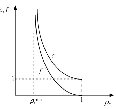
Coefficients c and f are functions of the relative density ρr. They verify c(1) = 1 and f(1) = 0 (fig. 1), so that the classical definition of the von Mises equivalent stress is obtained for the dense material.
Assuming an associated plasticity flow rule, it can be shown [17] that the corresponding expression of the equivalent plastic strain rate is:
2 / 1 2 ) (Tr 9 2 9 1 : 3 2 1 − + ρ = ε pl pl pl r c f c ε ε
ε& & & & 2 / 1 2 ) (Tr 9 1 : 3 2 1 + ρ = pl pl pl r c f ε e
e& & & (3) where ε& is the plastic strain rate tensor and pl e& its deviatoric part. In addition, the pl
volumic power of plastic deformation is given by:
ε σ ρ = ε σ = & & & r pl ij ij pl ε σ: (4)
The assumption of associated flow rule may be criticized in the field of cold metal compaction, due to the important contribution of grain rearrangement in the global plastic deformation of the medium. However, during hot powder forging, the powdered metal has already been cold pre-compacted, so that it exhibits a rather large initial relative density (typically 0.75 to 0.85), preventing from significant grain rearrangement. In this context, the normality rule holds and the first extension of the above compressible plasticity concepts to compressible viscoplasticity has been proposed by Abouaf et al. [1]. In this case, a relationship between the equivalent stress and the equivalent strain rate is substituted for the notion of instantaneous plasticity criterion. If the dense metal obeys a viscoplastic flow rule of the type:
) , ( T g σ = ε& (5)
where T is the temperature and the equivalent stress and strain rate are defined in the von Mises sense, then the average continuous medium representing the porous metal obeys the extended form:
) , ( T g rε= σ ρ & (6)
with σ and ε& defined according to (1) and (3). Here we shall assume that the dense material obeys the purely viscoplastic Norton-Hoff law:
m K / 1 3 3 1 σ = ε& (7)
where K is the metal consistency and m the strain rate sensitivity coefficient, both being temperature dependent. Hence, the one-dimensional constitutive equation of the porous metal can be written, according to (6):
m r K / 1 3 3 1 σ = ε ρ & or σ=K 3
(
3ρrε&)
m (8) In order to derive the three-dimensional constitutive equation, the viscoplastic potentialϕ
is introduced:(
)
1 3 1 + ε ρ + = ϕ m r m K & (9) Then, the stress tensor is obtained as follows:ε ε σ & & & & ∂ ε ∂ ε ∂ ϕ ∂ = ∂ ϕ ∂ =
(
)
− + ε ρ = − ε (Trε)I 9 2 9 1 3 2 33 & 1 & & c f c K r m
(
)
+ ε ρ = − e (Trε)I 9 1 3 2 33 & 1 & & f c
K r m (10)
where I denotes the identity tensor. Strain hardening and temperature softening effects can be taken into account, by use of the following law:
β ε + ε = T K K ( )nexp 0 0 (11)
where β is the temperature softening coefficient, ε0 and n are the strain hardening coefficients, K is a material parameter and 0 ε is the viscoplastic equivalent strain
defined by:
∫
ε = ε t u du 0 ( ) & (12) 2.2 Friction ModelRegarding hot forming of dense metals, sliding contact along tooling surfaces is often modelled using a viscoplastic friction law. The tangential shear stress vector τ is then related to the relative velocity vg by the following power law:
g p g f K v v n n σn σn τ = −( . ) =−α −1 (13) where α and p are friction coefficients, n is the normal vector at the tool/workpiece f interface, and vg is the relative velocity between the metal and the die, whose velocity is denoted vdie: n n v v v v v (( ). ) die die g = − − − (14)
In the case of hot forming of porous metals, this suggests using the same friction model, but with friction coefficients α and p possibly dependent on the relative density of f the material. Hence, the friction shear stress vector τ also derives from the following potential: 1 1 + + α = ϕ pf g f f p K v and v τ ∂ ϕ ∂ − = f (15) 2.3 Heat Transfer
Since the forming is performed under hot environment, the temperature evolution has to be modelled during the process. However, the thermal conductivity of porous media is known to decrease with porosity. In the literature, different models have been proposed: see the review of Cheng and Vachon [6]. These authors found, by comparing theoretical predictive models with experimental measurements, that convection and radiation which occur in the pore spaces can be neglected for small pore size and low or intermediate temperature. Despite the rather high temperature encountered in powder hot forging, the same assumption will be done in the present work, as a first approach. The thermal conductivity is then given by:
dense rk
where kdense is the thermal conductivity of the dense metal.
The energy balance equation due to heat transfer includes Fourier standard conduction law: ε σ: & ) .(k T r dt dT cp =∇ ∇ + ρ (17)
where ρ is the specific mass of the porous metal (ρ=ρdenseρr), c is the specific heat p of the metal (independent on ρr), dT/dt is the material or total derivative of temperature with respect to time, k is the thermal conductivity (equ. 16), r is the fraction of the deformation energy which is really transformed into heat. In the sequel, r will be assumed equal to 1.
The boundary ∂Ω of the processed material is basically subjected to two different types of thermal boundary conditions, depending whether contact with die is established or not. The boundary ∂Ω will then be split into a partition ∂Ω=∂Ωc∪∂Ωs, where ∂Ωc is the part of the boundary contacting dies whereas ∂Ωs is the free surface. The following boundary conditions apply on these regions.
• Convection and radiation on ∂Ωs:
) ( ) ( . 4 4 ext r r ext cv T T T T h T k∇ = − +ε σ − − n (18)
where T is the external temperature, ext h the convection coefficient, cv εr the material emissivity, σr the Stefan-Boltzmann constant and n the outward normal vector. When convection and radiation occur simultaneously equation (18) can be expressed:
) ( . hcr T Text T k∇ = − − n (19) ) )( ( with 2 2 ext ext r r cv cr h T T T T h = +ε σ + + (20)
In the context of non steady state time incremental computations, this permits a linearisation of the radiation law by using the value of temperature which comes from the previous time increment in (20).
• Conduction and additional friction flux on ∂Ωc: f die cd T T h T k∇ = − −φ − .n ( ) (21)
where hcd is the heat transfer coefficient between die and workpiece, Tdie the die
surface temperature, and φf the inward friction flux corresponding to the splitting of
quadratic approximation of the temperature profile in the normal direction [26], the expression of φf is: 1 + α + = φ pf g die f K b b b v (22)
in which b is the effusivity (b= kρcp ) and b the effusivity of the die material. die
2.4 Mass conservation
The evolution of the relative density is governed by the mass conservation equation:
0 Tr = ρ + ρ ε & r r dt d (23) where dρr /dt is the material or total derivative in time of the relative density.
3 FINITE ELEMENT RESOLUTION OF THE MECHANICAL PROBLEM 3.1 Problem Statement
At time t, the mechanical equations can be summarised as follows, neglecting gravity and inertia forces:
0 . = ∇ σ on Ω
(
)
+ ε ρ = − e ε I σ (Tr ) 9 1 3 2 33 & 1 & & f c K r m on Ω d T σn= on s Ω ∂ (24) g p g f K v v τ =−α −1 on c Ω ∂ 0 ). (v−v n= die on ∂Ωc
It should be noted that, in practice, the module of prescribed stress vector Td on the
"free" surface is equal to the atmospheric pressure and can be neglected with respect to internal stresses. However, it will be kept in the equations for generality.
Let us define the following spaces:
{
2 2 3}
1(Ω)= q∈L (Ω) ∇q∈(L (Ω))
{
∈ H Ω − die = ∂Ωc}
= ϑ v ( 1( ))3 (v v ).n 0 on (26){
∈ H Ω = ∂Ωc}
= ϑ ( 1( ))3 . 0 on 0 v vn (27)ϑ is the space of "kinematically admissible" velocity fields and ϑ0 is the space of "zero kinematically admissible" velocity fields. The virtual power principle states that the solution velocity field v∈ϑ should fulfill the following condition:
0 * . * . * : *∈ϑ0 − − = ∀
∫
∫
∫
Ω ∂ Ω ∂ Ω c s dS dS dV τv Td v ε σ v & (28)This is equivalent to say that the solution velocity field, v, should minimise the following functional Φ on the space of kinematically admissible velocity fields ϑ:
∫
∫
∫
Ω ∂ Ω ∂ Ω − ϕ + ϕ = Φ s c dS dS dV d f T v v) . ( (29)A more detailed expression of the functional Φ is: ⌡ ⌠ − + + = Φ Ω + + dV c f c m K m m ( 1)/2 2 1 ) (Tr 9 2 9 1 : 3 2 1 ) 3 ( )
(v ε& ε& ε&
∫
Ω ∂ Ω ∂ + − ⌡ ⌠ + α + s c f dS dS p K p d g f v T v . 1 1 (30) 3.2 Choice of a FormulationA flow formulation with the velocity field as unknown can be straightforwardly derived from this functional [7]. However, as already said, its main drawback is that it yields erroneous pressure and stresses values and can exhibit spurious velocity fields or become inaccurate when some regions of the domain Ω reach a fully dense state. Since in hot powder forging, the part is supposed to be fully densified at the end of the process, a mixed formulation passing the Brezzi-Babuska compatibility condition [5, 23] has to be developed.
Two approaches of a mixed two-field formulation are possible: the first one is the velocity-pressure (v,pH) formulation and the second one is the velocity-volumetric strain rate (v,θ&) formulation.
The velocity-pressure formulation consists in solving the equilibrium equation (28) under the constraint of the volumetric equation, issued from (10):
(
)
ε σ 3 & Tr& 3 Tr 3 1 −1 ε ρ − = − = m r H f K p (31)Consequently, the mixed problem can be written: ), ( ) , ( Find p ∈ϑ×L2 Ω H v such that ( *, *) 2( ), 0× Ω ϑ ∈ ∀ v p L
(
)
∫
= ε ρ + = − − − Ω − Ω ∂ Ω ∂ Ω Ω∫
∫
∫
∫
0 Tr ) 3 ( 3 * 0 * . * . * Tr * : ) ( 1 dV K fp p dS dS dV p dV m r H d H s c ε v T v τ ε ε v s & & & & (32)where *ε& is the virtual strain rate tensor associated with any virtual velocity field *v . Because of the non-linearity of the constraint equation (32b), it can be seen that the derived discrete velocity-pressure formulation would result in a non symmetric tangent stiffness matrix. This is the case in the similar mixed velocity-pressure approach developed by Jinka and Lewis [22].
• Velocity-volumetric strain rate formulation
The additional constraint to the equilibrium equation (28) is now given by θ& =Trε&, and
the corresponding mixed formulation is the following. ),
( )
, (
Find v θ& ∈ϑ×L2 Ω such that ( *, *) 2( ), 0× Ω ϑ ∈ θ ∀ v & L = θ − θ = − − θ
∫
∫
∫
∫
Ω Ω ∂ Ω ∂ Ω 0 ) (Tr * 0 * . * . * : ) , ( dV dS dS dV s c d & & & & & ε v T v τ ε v σ (33)Once again, the tangent stiffness matrix is found non symmetric. It should be noted, however, that when the volumetric strain rate θ& is chosen constant per element, using for example P1/P0 quadrangles or P2/P0 triangles in two-dimensional problems, θ& can be eliminated from (33b) at the element level [18, 14], its value being injected in the equilibrium equation (33a). This equation can then be solved for the velocity field only, using again a non symmetric tangent stiffness matrix. In the frame of three-dimensional problems, using linear tetrahedra such as in FORGE3®, such a formulation cannot be used and the global resolution for v and θ& should be carried out with a non symmetric matrix.
Non-symmetry might be more or less acceptable when using iterative solvers, although it implies somewhat more storage and computational effort per iteration. However, it has been preferred to develop a three-field formulation. As explained hereafter, it results in a symmetric tangent stiffness matrix and permits a minimal storage requirement as compared to previous formulations.
3.3 Three-Field Formulation
The three-field formulation consists in introducing an additional variable in order to obtain a symmetric tangent stiffness matrix. This variable must permit the formulation of the problem with a Lagrangian function. As the relative density directly depends on the volumetric strain rate (23), the volumetric strain rateθ& is the variable to be added. Firstly, Φ is rewritten as a function of v and θ&, on ϑ×L2(Ω):
⌡ ⌠ θ − + + = θ Φ Ω + + dV c f c m K m m ( 1)/2 2 1 9 2 9 1 : 3 2 1 ) 3 ( ) , ( ~ & & & & ε ε v
∫
Ω ∂ Ω ∂ + − ⌡ ⌠ + α + s c f dS dS p K p d g f v T v . 1 1 (34) Secondly, a weak form of the constraint θ& =Trε& is written:∫
*( Tr ( )) 0 ) ( *∈ 2 Ω θ− = ∀ Ω dV p L p & ε& v (35)Finally, the following Lagrangian L(v,θ&,p) is defined on ϑ×(L2(Ω))2, in which p is a
field of Lagrange multipliers of the constraint:
∫
Ω θ− + θ Φ = θ p p dVL(v,&, ) ~(v,&) (& Trε&(v)) (36) The stationarity of the Lagrangian L with respect to p (i.e. ∂L/∂p=0) ensures the fulfilment, in a weak form, of the constraint relation θ& =Trε&. Once this is achieved,
) , ( ~
θ
&v
Φ can be considered equal to Φ(v). Again the stationarity of the functional Φ(v)
with respect to v leads to the principle of virtual work (see [7] for a detailed demonstration).
Moreover, it can be shown [14] that the relation between the effective hydrostatic pressure p and the Lagrange multiplier p is: H
(
3 &)
Trε& 3 2 −1 ε ρ + = m r H c K p p (37)When the material approaches the dense state, then Trε&→0 and
H
p
p→ : the Lagrange multiplier p, is in this case nothing but the hydrostatic pressure.
The additional condition of non-penetration of forming tools (the solution velocity field v must be kinematically admissible in the sense of (26)) can be enforced by different methods, among which the penalty method which is used in software FORGE3® [8, 9,
15]. This method consists in adding a complementary term to the Lagrangian L, which will finally be written on (H1(Ω))3×(L2(Ω))2:
∫
∫
Ω ∂ Ω θ− + χ − + θ Φ = θ c dS dV p p L p die 2 2 1 ). ( )) ( Tr ( ) , ( ~ ) , ,(v & v & & ε& v v v n (38) where
χ
p is a large positive constant and denotes the Mac Cauley's bracketing (i.e.2 / ) (x x x = + ).
3.4 Finite Element Discretization
In powder forging, the material undergoes large deformations. Remeshing is required in order to avoid severely distortion of the finite element mesh. As reliable three-dimensional automatic remeshing procedures are based on linear tetrahedra, this kind of element is recommended here. In order to satisfy the Brezzi-Babuska compatibility condition, a three-field version of the P1+/P1 element [3, 13] has been developed and is presented hereafter. This choice has been fixed following a previous investigation of P2/P1 10-noded element [21], but which proved too computationally expensive.
In the P1+/P1 element, the velocity field is quasi-linear continuous, including additional degrees of freedom at the centre of gravity of the element (bubble formulation). It can be decomposed in two parts: a linear one, resulting from linear interpolation between the four apex velocities, and a complementary one issued from interpolation of velocity correction degrees of freedom defined at the centre of the element:
) ( ) ( ) (b l b k k N N V b v v v= + = + (39)
In (39), N denotes the linear interpolation function associated to apex k, k Vk is the
velocity vector at node k and the summation is extended to the four apexes (k = 1, 4) of the tetrahedron. Vector b is the vector of velocity corrections at element centre. The value of the "bubble" interpolation function N(b) is 1 at the centre and 0 on the element
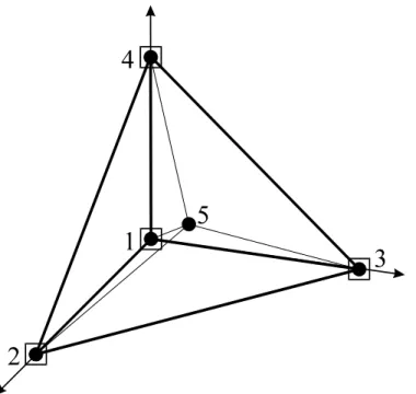
boundary (i.e. the four facets). This function is defined separately on each of the four sub-tetrahedra (the three nodes of each facet, plus the central node), so that the velocity field v is linear on each sub-tetrahedron (fig. 2).
On another hand, the field of Lagrange multipliers p and the volumetric strain rate field
θ& are linear continuous. Inside each finite element, we have:
k kP
N
p=
θ
&= NkΘ
&k (40) both summation being extended to the four apexes (k = 1, 4) of the tetrahedron. Let us denote V the global vector of nodal velocities (vector of 3Nbnoe components), B the global vector of central velocity corrections (3Nbelt components), P the global vector of nodal Lagrange multipliers (Nbnoe components) and Θ& the global vector of nodalvolumetric strain rates (Nbnoe components). The previous interpolations (39-40) are extended to the whole finite element mesh, by writing:
q b q n n N N V B v = + ( ) n nP N p= θ& =Nn
Θ
&n (41) where index n varies from 1 to Nbnoe (total number of apexes of tetrahedra) whereas index q varies from 1 to Nbelt (total number of elements). In (41) the interpolation functions have been extended to the whole mesh, Nk( x) (respectively Nq(b)(x)) havinga zero value when x is outside the elements the node k belongs to (respectively outside element q).
The discrete finite element Lagrangian is written as L(V,B,Θ&,P). Its stationarity condition provides the following system of non linear equations to be solved:
= ∂ ∂ = ∂ ∂ = ∂ ∂ = ∂ ∂ 0 0 0 0 P Θ B V L L L L & (42)
The discretized equations of this system are expressed hereunder:
Nbnoe k 1, 3 , 1 ∀ = = λ ∀
∫
∫
Ω ∂ λ Ω λ Ω λ − λ − − ⌡ ⌠ ρ ε = ∂ ∂ s dS N T dV P N dV c K V L n d n m m n m r n ) Tr( : ) 3 ( 2 1 B B ε& & 0 ) ( , , 1 = − χ − α +∫
∫
Ω ∂ λ µ µ µ Ω ∂ λ − c c f dS N n n v V N dS N v K vg p g n p m m die n (43) Nbelt q 1, 3 , 1 ∀ = = λ ∀0 ) Tr( : ) 3 ( 2 1 ( ) ( ) = − ⌡ ⌠ ρ ε = ∂ ∂
∫
Ω λ Ω λ − λ dV P N dV c K L b q m m b q m r q B B ε B & & (44) 0 9 2 9 1 ) 3 ( 3 , 1 1 = ⌡ ⌠ + − ε ρ = ∂ ∂ = ∀ Ω − N N P dV c f K N L Nbnoe n n r m m m m m nΘ
Θ
& & & (45)(
)
[
]
∫
Tr( ) Tr( ) 0 , 1 = − + ( ) = ∂ ∂ = ∀ Ω λ λ λ λ dV B V N N P L Nbnoe n q b q m m m m n n B BΘ
& (46)In the previous equations, repeated indices m and q varies from 1 to Nbnoe and from 1 to Nbelt respectively; B and B(b) are the discrete differential operators defined by:
n n Vλ λ = ∂∂ ε& B or, in components, δ ∂ ∂ + δ ∂ ∂ = ∂ ∂ = λ λ λ λ j i n i j n n ij n ij x N x N V ε 2 1 & B (47) q b q Bλ λ = ∂∂ ε& ) ( B or, in components, δ ∂ ∂ + δ ∂ ∂ = ∂ ∂ = λ λ λ λ j i b q i j b q q ij b q ij x N x N B ε ( ) ( ) ) ( 2 1 & B (48)
It should be noted that the integrals in (43-46) have to be computed on the sub-tetrahedra when they involve the "bubble" interpolation function N(b) or its spatial
derivative.
Let us use the following global notation for the set of non linear equations (42): 0
= ∂
∂L/ Y with Y =(V,B,Θ&,P). It is solved using a Newton-Raphson method. At each iteration of the method, the equations are linearised and a correction
) , , , ( V B Θ P Y
δ
δ
δ
δ
δ
= & is computed to improve the current estimate Y: ) ( ) ( 2 2 Y Y Y Y Y ∂ ∂ − = ∂ ∂ L Lδ
(49)This is worth noting that, according to the definition of the bubble interpolation function, the stationarity equations (44), which correspond to the derivation of L with respect to the additional velocity degrees of freedom B, can be written on each element in a decoupled manner. Consequently, the Newton-Raphson correction Bδ can be eliminated at element level by writing, in each element e:
) ( ) ( e e L e L Y B Y Y B Y ∂ ∂ − = ∂ ∂ ∂ ∂
δ
(50) While assembling the tangent stiffness matrix ∂2L/ Y∂ 2, this permits to expressδ
Be inabout four to five times more tetrahedra than nodes (apexes) in a three-dimensional tetrahedral mesh, this elimination proves quite efficient. After elimination of these degrees of freedom, the system to be solved can be written as:
) ' ( ' ) ' (Y Y G Y H
δ
=− (51)where
δ
Y'=(δ
V,δ
Θ&,δ
P). In practice, the vector Y' is partitioned into Nbnoe blocks,each block containing the four primary nodal unknowns.
This linear system is solved with a general minimum residual method [24, 25], as in the standard incompressible viscoplastic formulation in FORGE3®, except that in the
present case, it has been extended to the solution of a system with five unknowns per node (instead of four). A block-diagonal preconditioning is used and is designed as follows. After elimination of additional velocity degrees of freedom, the matrix H of the system (51) has the following structure:
( )
( ) ( )
pp T p T vp p T v vp v vv H H H H H H H H H θ θ θθ θ θ (52)The block diagonal preconditioning matrix C, which is required to be definite positive and to approach the inverse of H is then composed of Nbnoe diagonal blocks C(n), of size 5×5, whose non zero terms are:
(
)
= = = = − pp nn n nn n n n vv n H C H C µ λ H C 1 1 3 1, , for ) ( ) ( 55 ) ( 44 1 ) ( θθ µ λ λµ (53)It can be noted in particular that such a block-diagonal preconditioning can remedy the ill-conditioning issued from the penalty method for contact. As a matter of fact, a nodal penalty method is used in FORGE3®: the last integral in equation (38) is approached by a summation on nodes with application of repulsive nodal forces if nodes tend to penetrate the tooling [15]. Hence, such a method only produce diagonal terms in the tangent stiffness matrix. The resulting poor conditioning can be counterbalanced by the block-diagonal preconditioner and does not affect the convergence rate of the iterative solver.
An isoparametric continuous four node interpolation is used for the discretization of temperature, the finite element mesh being the same as for the mechanical resolution (except central nodes, not used here). In each tetrahedral element, we have:
k kT
N
T = (54)
the summation being extended to the four apexes (k = 1, 4) of the tetrahedron The use of this discretization in the variational form of equation (17), according to the Galerkin finite element method, leads to the following classical set of non linear differential equations in which T is the global vector of nodal temperature (Nbnoe components).
F KT T C + = dt d (55) C is the heat capacity matrix, K the conductivity matrix and F the thermal loading vector. It should be noted that using a moving mesh formulation, dT/dt is here nothing but the partial derivative in time of the vector of nodal temperatures, since the nodes are convected with the material flow (see the scheme for configuration updating in section 5).
The expressions of matrices C and K and of vector F are as follows:
∫
Ω ρ = c N N dV Cnk p n k (56)∫
∫
∫
Ω ∂ Ω ∂ Ω + + ∇ ∇ = c s dS N N h dS N N h dV N N k Knk n k cr n k cd n k (57)∫
∫
∫
Ω ∂ Ω ∂ Ω φ + + + = c s dS N T h dS N T h dV NFn σ: ε& n cr ext n ( cd die f) n (58)
where n and k vary between 1 and Nbnoe.
The first order differential equation (55) is solved using a second order three level (two step) finite difference scheme [19]. Given two successive time steps ∆t1 and ∆t2 (not necessarily of same size), the nodal temperature vector T and its time derivative dT/dt are expressed as:
2 1 3 2 1 t−∆t +α t +α t+∆t α = T T T T (59) 2 1 2 1 ) 1 ( t g t g dt d t t t t t t ∆ − + ∆ − − = T T −∆ T +∆ T T (60)
where α1,α2,α3andg are numerical coefficients providing different integration schemes. In fact, such schemes are second order accurate on condition that [19]:
∆ ∆ + − ∆ ∆ α − + α − = α 2 1 2 1 1 1 2 1 2 ) 2 1 ( ) 1 ( t t g t t (61) and ∆ ∆ + + ∆ ∆ − α = α 2 1 2 1 1 3 1 2 ) 2 1 ( t t g t t (62) It can be noted that α1 +α2 +α3 =1 and that each scheme is determined by only two parameters, for instance α1 and g. Moreover, such schemes are unconditionally stable
(no limitation on ∆t) on condition that [19]:
) 1 ( 2 1 and 2 1 1 g g ≥ α ≥ − (63)
As regards matrices C, K and F, equation (59) is not used because it would result in an iterative resolution of (55). This is avoided by using a linearisation technique, suggested by Zlamal [27] and shown to be second order accurate [26], each non linear matrix W (C, K or F) being expressed as:
− ∆ ∆ + α + α + α = −∆1 ( −∆1) 1 2 3 2 1 t t t t t t t t t W W W W W W (64)
which yields, after injection of (61) and (62), the following simple expression:
t t t t t g t t g W W W ∆ ∆ + + + ∆ ∆ + − = −∆ 1 2 1 2 1 2 2 1 1 2 2 1 1 (65)
Finally, the injection of the time discretization defined by equations (59-60) in equation (55) results in a linear system
B
ATt+∆t2 = (66)
to be solved for the unknown nodal temperature vector Tt+∆t2. In practice, we use the two-step implicit scheme (α1 =0, g =3 2). It can be noted that this scheme is different from the one-step backward Euler implicit scheme (the expression of the time derivative is different, which yields to second order accuracy). For the first time increment, a one-step Crank-Nicolson scheme is used (α1 =0,α2 =α3 =12, g =1).
When there is a large temperature difference between the workpiece and the forging dies, space and time numerical oscillations are observed, whatever the integration scheme used. To overcome this numerical problem, a classical remedy is to approach C by its diagonal lumped form CL:
∫
Ω ρ δ = c N dV CL mn p m mn (67)where index m is not summed. However, this approximation is not always efficient enough, more particularly using three-dimensional tetrahedral elements. The size of the thermal time step is then chosen with a different value from that of the mechanical time step, so that it remains greater than the critical value ∆tcissued from the Courant limit [12]: k l c tc p 32 ∆ ρ = ∆ (68)
where ∆l is a reference length which is computed as the distance between neighbouring nodes along the normal direction to the workpiece/die interface.
5 THERMO-MECHANICAL COUPLING AND CONFIGURATION UPDATING
There is a thermomechanical coupling between mechanical equations (24), and heat transfer equations (17-22). However, the material flow does not strongly depends on temperature, so there is no need to solve these problems simultaneously at each time increment [t, t+∆t]. A staggered coupling algorithm is preferred. At any time t, the temperature field, Tt is assumed to be known. It allows the calculation of the
consistency of the material (11) and then the computation of the flow. Once the velocity field is known, at time t, the internal source of heat due to deformation (4) and to friction (22) are calculated, allowing the computation of the temperature field at time t+∆t.
The configuration is then updated, according to a Euler explicit scheme. Denoting X the global vector of nodal coordinates, we have:
t t
t
t X tV
X +∆ = +∆ (69)
The same scheme is applied to the mass conservation equation to express the evolution of nodal relative density. Let R denote the vector of nodal relative densities (components Rn,n=1, Nbnoe).
) 1 ( ) exp( t n t n t n t n t t n R t R t R +∆ = −∆
Θ
& ≈ −∆Θ
& (70) A strict application of (70) would yield relative density values slightly greater than 1 as the material becomes fully dense. To prevent this, the upper limit of 1 is applied.More generally, the previous procedures have been implemented in the software FORGE3®. In addition, an automatic remeshing procedure is triggered when necessary
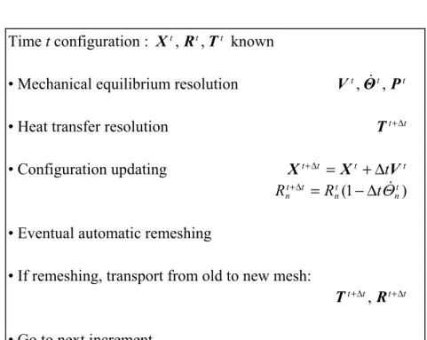
in order to avoid mesh degeneration. In case of remeshing, a transportation of nodal temperature and relative density values from old to new mesh is carried out by means of direct interpolation. The complete incremental resolution scheme is given at figure 3. 6 VALIDATION
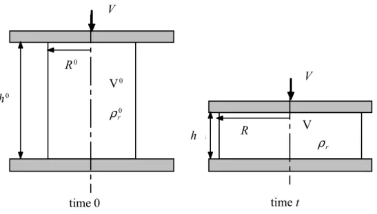
In order to validate the three-field formulation, the reference solution of a uniaxial free compression test (fig. 4) has been established. It is possible to exhibit a closed form solution, on condition that coefficients c and f are kept constant. Under this assumption, the following solution has been derived (details are given in appendix):
c f f r r h h + − ρ = ρ 3 0 0 (71) m m h V f c K + − = σ + 2 1 3 (72) in which h and h denote the initial and current height of the compacted specimen, 0 0
r
ρ
and ρr are the initial and current relative density, V is the compaction prescribed velocity (which is not necessarily constant). The other coefficients are those used in the above presentation.
The values that have been used for the comparison are: h = 120 mm, V = 3 mm.s0 -1, ρ0
= 0.80, K = 100 MPa.sm, m = 0.25. Coefficients c and f are kept constant (c = 6.463, f =
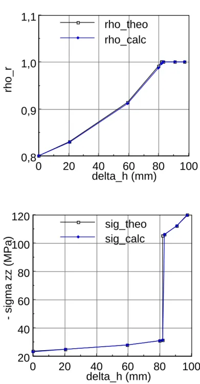
0.45) until the full densified state is reached. Then the corresponding values c = 1 and f = 0 are used, as they are associated with dense state. In such conditions, a uniform dense state is reached for h = 38.3 mm (height reduction ∆h = 81.7 mm). The agreement between the finite element solution and the analytic one is excellent for both relative density and stress values (fig. 5). This is observed before full densification, as well as after, when the deformation becomes purely viscoplastic and incompressible. The discontinuity of the stress evolution is clearly a consequence of the abrupt change in the values of coefficients c and f at full densification. The error on the axial stress
(respectively the relative density) is less than 0.13% (respectively 0.40%) up to the end of the test, corresponding to a cylinder height of 20 mm.
7 APPLICATION
The finite element model has been applied to the simulation of the hot compaction step of a connecting rod preform, made of aluminium alloy, in order to test the ability to simulate a complex three-dimensional compaction process. The preform is normally obtained by a cold compaction step. Since this first step has not been simulated, the thickness of the preform has been taken uniform along the compaction direction z (fig. 6). For the same reason, its initial relative density distribution has been assumed uniform, equal to 0.80. Figure 6 shows the initial volumic mesh of the preform (initially rather coarse) as well as the surfacic meshes of the tooling components in initial position. The tooling is composed of a lateral die, two cylindrical dies at both ends of the rod and a punch which has a prescribed vertical velocity. For symmetry reason, only one quarter of the part is effectively computed. The process and material parameters used in the computation come from previous experimental work [16] and are given in table 1.
Figure 7 illustrates the progress of the forming. It can be seen that the preform is first deformed in its central I-beam region. Then the deformation extends to the small end (piston end) and to the big end (crankshaft end). This figure also reveals the efficiency of the remeshing procedure, resulting in a finer discretization in regions of small curvature radii.
As expected with such an initial preform geometry, densification occurs first in the central region (fig.8), and then extends to the piston end and the crankshaft end. This can be seen on figure 9, on which distributions of relative density have been plotted in five transverse sections along the connecting rod, at an intermediate stage of compaction. The compaction of the centre of the arm of the rod is associated to some de-densification near the zone contacting the punch. The dilatation (or de-densification) affects the free surface zone near the punch edge. A similar phenomenon occurs in the big end region where the outer zone is first compacted: there is a rapid densification of the material under the punch and some de-densified material beside, near the inner radius.
Figure 10 shows the configuration reached near the end of the compaction process. At this stage, the preform has been almost completely compacted. The last region to be densified is located at the crankshaft end. The de-densification phenomena are significant in this region, the relative density being even noticeably lower than the
initial value of 0.80. Such a non uniform compaction could be avoided by defining a preform of non uniform thickness or/and relative density (this is actually the case in real production).
Finally, figure 11 shows the temperature distribution at the end of the process. The competition between heat loss at tool contact and heat dissipation by plastic deformation and friction results in a maximum temperature drop of about 60°C. It can be seen that some regions near both ends of the rod suffer from significant temperature inhomogeneities which could induce deformations and residual stresses after cooling. The complete simulation took 80 increments, 26 remeshing operations and about 15 hours (CPU time) on IBM-Risc6000-43T, the maximum number of nodes being about 5000. Finally, the relative variation of the material mass is only 0.038% at the end of the computation.
CONCLUSION
A new three-field formulation (velocity, volumetric strain rate and pressure) has been developed for an accurate simulation of the hot forging of metal powder. The finite element discretization is based on the new linear tetrahedral P1+/P1/P1 element. It has been implemented in the computation code FORGE3®, whose iterative solver has been adapted to the resolution of non linear systems with five nodal unknowns. The finite element resolution of the three-dimensional mechanical problem has been coupled in a staggered manner with the heat transfer resolution, providing an efficient tool for the simulation of hot powder compaction processes. This has been illustrated by treating the hot forging of a connecting rod preform. In the future, such a formulation should be extended to the modelling of cold compaction, in order to simulate the global powder forming process.
ACKNOWLEDGEMENT
The present study has been conducted in the frame of a European Brite/Euram project : BRE2 CT 92-0220 with RENAULT and PEAK as industrial partners.
REFERENCES
[1] M. Abouaf, J.L. Chenot, G. Raisson and P. Bauduin, Finite element simulation of hot isostatic pressing of metal powders, Int. J. Num. Meth. Eng. 25 (1988) 191-212.
[2] C. Aliaga and E. Massoni, 3D numerical simulation of thermo-elasto-visco-plastic behaviour using stabilized mixed F.E. formulation: application to heat treatment, Proc. Numiform'98, Simulation of Materials Processing: Theory, Methods and Applications, J.Huétink and F.P.T.Baaijens (eds.) (1998) 263-269.
[3] D.N. Arnold, F. Brezzi and M. Fortin, A stable finite element for Stokes equation, Calcolo 21 (1984) 337.
[4] M.J.M. Barata Marques and P.A.F. Martins, Finite element simulation of powder metal forming, J. Mat. Process. Tech. 28 (1991) 345-363.
[5] F. Brezzi, On the existence, uniqueness and approximation of saddle-point problems arising from Lagrangian multipliers, RAIRO Num. Analysis R2 (1974) 129-151.
[6] S.C. Cheng and R.I. Vachon, A technique for predicting the thermal conductivity of suspensions, emulsions and porous materials, Int. J. Heat Mass Transfer 13 (1970) 537-546.
[7] J.L. Chenot, F. Bay and L. Fourment, Finite element simulation of metal powder forming, Int. J. Num. Meth. Eng. 30 (1990) 1649-1674.
[8] J.L. Chenot, T. Coupez and L. Fourment, Recent progresses in finite element simulation of the forging process, in: Proc. COMPLAS IV, 4th Int. Conf. on Computational Plasticity, D.R.J.Owen & E.Onate (eds.), Pineridge Press, Swansea (1995) 1321-1342.
[9] J.L. Chenot, T. Coupez, L. Fourment and R. Ducloux, 3-D finite element simulation of the forging process: scientific developments and industrial applications, in: Proc. ICTP, Int. Conf. on Technology of Plasticity, T.Altan (ed.) (1996) 465-474.
[10] T. Coupez, A mesh improvement method for 3D automatic remeshing, Numerical Grid Generation in Computational Fluid Dynamics and Related Fields, N.P.Weatherhill, P.R.Eiseman, J.Haüser and J.F.Thompson (eds.) (1994) 615-624.
[11] T. Coupez and S. Marie, From a direct solver to a parallel iterative solver in 3-D forming simulation, Int. J. Supercomput. Appl. 11 (1997) 277-285.
[12] G. Comini and M. Manzan, Stability characteristics of time integration schemes for finite element solutions of conduction-type problems, Int. J. Num. Meth. in Heat and Fluid Flow 4 (1994) 131-142.
[13] M. Fortin and A. Fortin, Experiments with several elements for viscous incompressible flows, Int. J. Num. Meth. Fluids 5 (1985) 911-928.
[14] L. Fourment and M. Bellet, Hot powder forging, in: Modelling of Welding, Hot Powder Forming and Casting, L.Karlsson (ed.), ASM International, chap. 7 (1997) 131-158.
[15] L. Fourment, K. Mocellin and J.L. Chenot, An implicit contact algorithm for the 3D simulation of the forging process, Computational Plasticity - Fundamental and Applications, Proc. Complas 5, 5th Int. Conf. on Computational Plasticity, Barcelona, D.R.J. Owen et al. (eds.), Pineridge Press, Swansea (1997) 873-877. [16] H. Grazzini, Etude expérimentale du comportement rhéologique de milieux
granulaires à constituants plastiquement déformables: comparaison de poudres de plasticine et d'alliages d'aluminium (Experimental study of the rheology of granular media composed of deformable plastic grains: comparison between plasticine powder and aluminium alloys), Ph.D. Thesis (in french), Ecole Nationale Supérieure des Mines de Paris, 1991.
[17] R.J. Green, A plasticity theory for porous solids, Int. J. Mech. Sci. 14 (1972) 215-224.
[18] K. Hans Raj, L. Fourment, T. Coupez and J.L. Chenot, Simulation of industrial forging of axisymmetrical parts, Eng. Comp. 9 (1992) 575-586.
[19] M.A. Hogge, A comparison of two and three level integration schemes for non linear heat conduction, in: Proc. Numerical Methods in Heat Transfer, R.W.Lewis et al. (eds.) (Wiley, 1981) 75-90.
[20] Y.T. Im and S. Kobayashi, Analysis of axisymmetric forging of porous materials by the finite element method, Advanced Manufacturing Processes 1 (1986) 473-499.
[21] A.G.K. Jinka, M. Bellet and L. Fourment, A new three-dimensional finite element model for the simulation of powder forging processes: Application to hot forming of P/M connecting rod, Int. J. Num. Meth. Eng. 40, (1997) 3955-3978.
[22] A.G.K. Jinka and R.W. Lewis, Finite element simulation of hot isostatic pressing of metal powders, Comp. Meth. Appl. Mech. Eng. 114 (1994) 249-272.
[23] J.T. Oden and G.F. Carey, Finite Element: Mathematical Aspects, vol. 4 (Prentice-Hall, Englewoods Cliffs, New Jersey, USA, 1984).
[24] Y. Saad, Practical use of some krylov subspace methods for solving indefinite and nonsymmetric linear systems, SIAM J. Sci. Stat. Comp. 5 (1984) 203-228.
[25] Y. Saad and M.H. Schultz, GMRES: a generalized minimum residual algorithm for solving nonsymmetric linear systems, SIAM J. Sci. Stat. Comp. 7 (1986) 856-869.
[26] N. Soyris, Modélisation tridimensionnelle du couplage thermique en forgeage à chaud (Three-dimensional modelling of thermomechanical coupling in hot forging), Ph.D. Thesis (in french), Ecole Nationale Supérieure des Mines de Paris, 1990.
[27] M. Zlamal, Finite element for non linear parabolic equations, RAIRO Num. Analysis 11 (1977) 93-107.
APPENDIX
The uniaxial compression of a compressible viscoplastic axisymmetric specimen is considered. The contact along tool surfaces is supposed perfectly sliding (no friction). The deformation is then homogeneous throughout the specimen. Denoting V the modulus of the compression velocity, the components of the strain rate tensor are:
h V zz =−
ε& ε&rr =ε&θθ (A1)
The stress tensor is diagonal, the only non zero component being σzz. Then the equivalent stress is, according to (1):
zz f c+ σ − = σ (A2)
Let us express now the deviatoric part and the volumetric part of the flow rule (10). This yields respectively:
e s = 2 ( 3ρ ε&)m−1&
r c
K
and Trσ= ( 3ρ ε&)m−1Trε&
r
f K
(A3) The flow rule (10) can then be inverted, using a combination of (A3) and (8):
) ) (Tr 2 3 ( 2 ) (Tr 3 1 I σ s I ε e ε r c + f σ ε ρ = +
= & & &
& (A4)
The application of (A4) to (A1a) yields:
zz r rr σ f −c σ ε ρ = ε = ε θθ (2 ) 2 & & & zz r zz σ c+ f σ ε ρ =
ε& &( ) (A5) Relation (A5b), combined with (8) and (A2) permits to obtain the analytical expression of the axial stress (72):
m m zz h V f c K + − = σ + 2 1 3 (A6) As regards the relative density evolution, it is obtained in the following way. The summation of the three strain rate components (A5), combined with (A1a) yields the expression of volumetric strain rate:
f c f h V + − = = ∇ =
Integration of (A7) can be achieved easily under the assumption of constant coefficients c and f during compaction. Denoting V and V the initial and current volume of the 0
specimen respectively, we have:
0 0 0 0 ln 3 3 ) ( V V ln h h f c f dt h V f c f du u t t + = ⌡ ⌠ + − = θ =
∫
& (A8)which yields finally relation (71):
c f f r r h h + − ρ = ρ 3 0 0 (A9)
It should be noted that equation (72) is not submitted to the restrictive condition of constant coefficients c and f, and that (71) and (72) hold for time dependent compression velocity V.
Notations
superscripts
(b) bubble part (of velocity field) d given or prescribed
(l) linear part (of velocity field) L lumped t time pl plastic 0 initial e relative to element e subscripts
die relative to die
dense relative to the dense material
g sliding (in relative sliding velocity between workpiece and die) k, m, n, q relative to node k, m, n, q
i, j,
λ
,µ
relative to components (spatial directions) b thermal effusivityB global vector of velocity correction degrees of freedom at element centroïd B discrete differential operator linking strain rates to nodal velocities
) (b
B ) discrete differential operator linking strain rates to velocity correction
degrees of freedom at element centroïd c coefficient of constitutive equation
p
c heat capacity
C heat capacity matrix
e& deviatoric part of the strain rate tensor f coefficient of constitutive equation F thermal loading vector
g coefficient of three-level finite difference scheme h specimen height
cd
h coefficient of heat exchange by conduction
cr
h coefficient of heat exchange by conduction and radiation
cv
h coefficient of heat exchange by convection I identity tensor
k thermal conductivity K viscoplastic consistency
0
K heat conductivity matrix
∆l characteristic length of the finite element discretization L Lagrangian
m strain rate sensitivity coefficient n outward unit normal vector Nbelt total number of elements Nbnoe total number of nodes
n
N interpolation function of node n
) (b q
N bubble interpolation function of centroid node q p Lagrange multiplier f p friction coefficient H p hydrostatic pressure k
P Lagrange multiplier value at node k
P global vector of nodal Lagrange multipliers
r fraction of deformation power transformed into heat R global vector of nodal relative densities
s deviatoric stress tensor t time
∆t time increment T temperature
ext
T external temperature
T vector of nodal temperatures T stress vector
v velocity vector v* virtual velocity field
V volume of the specimen of the uniaxial compaction test V velocity module in the uniaxial compaction test
V global vector of nodal velocities
k
V velocity vector of node k x position vector
X global vector of nodal coordinates Y global vector of unknowns
α friction coefficient
3 2 1,α ,α
α coefficients of three-level finite difference scheme
β temperature softening coefficient (in consistency expression)
ij
δ Kronecker symbol (= 1 if i = j ; = 0 if i≠ j) ε& strain rate tensor
*
ε& virtual strain rate tensor associated with v*
ε& equivalent plastic strain rate
0
r
ε radiation emissivity
f
φ inward friction flux in workpiece
ϕ viscoplastic potential
f
ϕ viscoplastic friction potential
Φ functional of velocity field for compressible viscoplasticity
Φ~ functional of velocity and strain rate fields for compressible viscoplasticity
p
χ penalty constant for non-penetration condition
Ω domain occupied by the workpiece
Ω
∂ domain boundary
c
Ω
∂ part of ∂Ω in contact with dies
s
Ω
∂ part of ∂Ω free from contact
θ& volumetric strain rate k
Θ
& value of volumetric strain rate at node kΘ& global vector of nodal volumetric strain rates
ρ specific mass
r
ρ relative density σ Cauchy stress tensor
σ equivalent stress
r
σ Stefan-Boltzmann constant τ friction stress vector
Captions
Fig. 1: Variation of coefficients c and f versus the relative density ρr (schematic). Fig. 2: P1+/P1/P1 tetrahedral element.
Fig. 3: Incremental resolution scheme. Fig. 4: Uniaxial free compression test.
Fig. 5: Comparison between finite element results and analytical solution. Plots of relative density and axial stress vs height reduction.
Fig. 6: Hot compaction step of a connecting rod preform made of aluminium alloy powder. Initial position of the volumic mesh of the preform and of the surfacic meshes of the tooling.
Fig. 7: Successive deformed configurations of the preform at 10, 20, 26 and 35% height reduction.
Fig. 8: Intermediate compaction stage (15% height reduction). Relative density distribution.
Fig. 9: Intermediate compaction stage (28% height reduction). Deformed mesh and distribution of relative density in five transverse sections of the preform.
Fig. 10: Distribution of relative density near the end of forming.
1
ρ
r
1
c
f
ρ
r
min
Figure 1: Variation of coefficients c and f versus the relative density ρr (schematic).
c
f
c, f
min rρ
ρ
rFigure 2: P1+/P1/P1 tetrahedral element.
v
Time t configuration : Xt, Rt,Tt known
• Mechanical equilibrium resolution Vt, &Θt, Pt
• Heat transfer resolution Tt+∆t
• Configuration updating Xt+∆t = Xt +∆tVt ) 1 ( t n t n t t n R t R +∆ = −∆
Θ
& • Eventual automatic remeshing• If remeshing, transport from old to new mesh:
t t t t+∆ R+∆ T , • Go to next increment
V0 V ρr time 0 time t h0 h R0 R V V ρr0
Figure 4: Uniaxial free compression test. V V h 0 h 0 R R 0 V r ρ 0 r ρ time t V
100
80
60
40
20
0
0,8
0,9
1,0
1,1
rho_theo
rho_calc
delta_h (mm)
rh
o
_
r
100
80
60
40
20
0
20
40
60
80
100
120
sig_theo
sig_calc
delta_h (mm)
-
s
ig
m
a
z
z
(
M
P
a
)
Figure 5: Comparison between finite element results and analytical solution. Plots of relative density and axial stress vs height reduction.
Table 1: process and material parameters used in the simulation Initial preform height 21 mm
Maximum height reduction 7.35 mm (35%) Punch velocity 100 mm.s-1 Initial temperature 600 °C Initial (uniform) relative density 0.8
64 . 0 1 36 . 0 − ρ ρ − = r r f f c=1+12.14 0 K =54.5 MPa.sm m = 0.25 K 4200 = β 2 . 0 = α 25 . 0 = f p 2700 = ρdense kg.m-3 1037 = p c J.kg-1.K-1 250 = dense k W.m-1.K-1 6000 = cd h W.m-2.K-1 200 = die T °C 11200 = die b J.K-1.m-2.s-1/2 20 = ext T °C 30 = cv h W.m-2.K-1 7 . 0 = εr