Analysis of variance impact on manufacturing flow time

(1)

ANALYSIS OF VARIANCE IMPACT ON MANUFACTURING FLOW TIME

by

Jackson Sheng-Kuang Chao

B.S. Electrical Engineering and Computer Science University of California, Berkeley (1986)

Submitted to the MIT Sloan School of Management and the Department of Electrical Engineering and Computer Science in

Partial Fulfillment of the Requirements for the Degrees of Master of Science in Management

and

Master of Science in Electrical Engineering and Computer Science at the

Massachusetts Institute of Technology May, 1991

distribute copies of this thesis in whole or in part.

Signature of Author Certified by Certified by Certified b Q

Signature

Accepted b --Accepted by

Signature redacted

May 17, 1991

Alvin W. Drake, Professor of Electrical Engineering

Signature redacted

Stephen C. Graves, beputy Dean, Professor of Management

I

Sgnature

redacted

A. Kochan, Professor of Management Jeffrey A.arks, Aoiatole s Bac s Programs

Signature redacted

Artfluft. Smith, Chair, Dep t~n(Ct-rMItte~-n Graduate Studies MASSACAUSETS INSTITUTE

OF TECHNOLOGY

JUN

2

4

1991

(2)

ANALYSIS OF VARIANCE IMPACT ON MANUFACTURING FLOW TIME

BY

Jackson Sheng-Kuang Chao

Submitted to the Sloan School of Management and the Department of Electrical Engineering and Computer Science on May 17, 1991 in Partial Fulfillment of the Requirements for the Degrees of Master of Science in

Management and Master of Science in Electrical Engineering

ABSTRACT

The cost accounting system at Boeing does not emphasize flow time, the time required by the production system to manufacture a product, as a significant manufacturing cost. Current emphasis on schedule adherence, along with close management attention to work station head count, encourage

production supervisors to maintain flow time and minimize head count. In this thesis, I show that flow time is a significant manufacturing cost and that exclusion of this cost has resulted in production decisions that over

emphasized head count reduction, at the expense of flow time.

I define flow time cost and examine three components of flow time cost: 1) inventory carrying cost, 2) revenue opportunity cost, and 3) variable capital cost. I show that including flow time cost in the management accounting system has significant implications on present production planning methodology.

After discussing flow time cost, I present a dual-prong strategy for flow time reduction. First, I propose a near term flow time reduction strategy through evaluation of potential trades of human and/or capital investments for immediate flow time reduction. This near term strategy reverses the effects of past production decisions that relied on head count to realize learning curve benefits. Next, I propose a far term flow time reduction strategy by evaluating the impact of system variances on manufacturing productivity. The analysis shows that for major shops within the manufacturing sequence, a number of "vital few" variances account for the majority of the effects on manufacturing productivity. Secondary cause-effect analysis shows that the Engineering organization has significant indirect impact on manufacturing productivity through its effects on these "vital few" variances. I propose an alternate resource allocation methodology based on the results of the

(3)

Next, I examine the importance of modifying the current incentive system for motivating the organization towards continuous flow time reduction.

Specifically, I propose that flow time cost be charged directly to the operating divisions and that it be incorporated as part of the management performance evaluation and reward system. I suggest that restructuring the incentive

system to include flow time cost will motivate cross functional

communication between the operations and engineering organizations and lead to significant near term and far term flow time reduction in the

manufacturing sequence.

The above recommendations, formulated with the insights and experiences of numerous Boeing engineers and managers, were presented to Boeing management and have received strong support. A planning directive has been issued at Boeing's Everett plant to implement these recommendations.

Thesis supervisors: Alvin W. Drake

Professor of Electrical Engineering and Computer Science

Stephen C. Graves

Leaders for Manufacturing Professor

Deputy Dean, Sloan School of Management Thomas E. Kochan

George Maverick Bunker Professor of Management

(4)

ACKNOWLEDGEMENTS

I gratefully acknowledge the support and resources made available to me through the Leaders for Manufacturing Program, a partnership between MIT and eleven major U.S. manufacturing companies.

To my friends at Boeing, thank you for being so supportive and helpful during the internship. Each of you have made my six-and-half months in Seattle a very special and enjoyable experience. In particular, special thanks to David Fitzpatrick and Fred Farnsworth, who generously shared their insights and knowledge and gave me their support.

To Professor Drake, whose support and courage made me a better, more confident student in life. To Professor Graves, whose insights and dedication gave this thesis its focus and substance (thanks again, Steve). To Professor Kochan, whose teachings influenced my thinking greatly on the importance of organizational relations.

My deepest gratitude to my parents, without whom all this would not mean

as much. Your presence gives me stability and strength. For all the times you have stood beside me, my heartfelt thanks to you both.

(5)

INTRODUCTION

1.1 Background

Boeing is the world's most successful airplane manufacturer. In 1990,

Boeing's family of commercial passenger airplanes' carried over 700 million passengers 2 to destination all over the globe. Boeing's over fifty percent market share of the worldwide airplane market continues to lead all other

airplane manufacturers.

The competitive positions in the industry, however, are evolving. While Boeing's chief competitor had historically been the McDonnell Douglas Corporation3, the past decade has seen the displacement of

McDonnell Douglas from the number two position in the airplane market by Airbus Industries, a consortium formed by four European governments

(England, Germany, France, and Spain). The financial support provided by these four governments to Airbus for the development and manufacturing of new airplanes has resulted in significant market gains for Airbus and made it a legitimate player in the industry. The rapid rate that Airbus has sustained in gaining market share during the 1980s highlights the importance that Airbus has placed on the commercial aviation industry and underlines its determination to become a key player in the airframe market.

1_The_{Boeing 707,}_{727, 737, 747,}_{757, 767 (the Boeing 777 will be introduced in 1994).}

2_{Cruze, Deane. Breaking Out of the Box, MANAGER}_-_{Boeing Management Magazine,}

Mar-April 1990.

3_{McDonnell Douglas presently produces the MD-80, DC-10 and MD-11 airplanes.}

(10)

Boeing though is not resting on its laurels. Current Boeing leadership is emphasizing the importance of continuous quality improvement (CQI) and has made it an explicit goal of the corporation to use CQI as the preferred way to improve product quality, customer service and corporate profitability. This commitment has also resulted in Boeing's participation in the Leaders for Manufacturing (LFM) program at the Massachusetts Institute of Technology. The Leaders for Manufacturing program, a joint effort between the

Massachusetts Institute of Technology and eleven industrial partners4 , has as its mission to educate future leaders for manufacturing and to improve U.S industrial competitiveness.

In this thesis, I present the results of my thesis internship at The Boeing Company. In June 1990, I started my internship at Boeing in the New Airplane Division5 to conduct research for a joint engineering and management thesis for the department of Electrical Engineering and the Sloan School of Management. My Boeing advisor recommended that I study the Boeing 767 final assembly process at Boeing's Everett, Washington plant to assimilate lessons learned about 767 manufacturing and to make specific recommendations for the 777 program.

I conducted my study at the Everett plant from July through mid-December of 1990. During those six months, I worked closely with various groups at the Everett facility (especially the Industrial Engineering group) and learned valuable lessons from the people around me. At the end of the

4_{The industrial partners are Alcoa, Boeing, Chrysler, Digital Equipment Corporation (DEC),}

General Motors, Hewlett-Packard, Johnson & Johnson, Kodak, Motorola, Polaroid, and United

Technology Corporation (UTC).

5

(11)

internship, we (I and all the people at Boeing who generously gave their time and support) formulated a set of three specific recommendations based on our six month study. These recommendations, detailed in chapters 3, 4 and 5, should not only have a positive impact on the Everett plant, but on the 777 division as well.

1.2 Thesis Summary

In this thesis I present results of my six-and-half month research internship at The Boeing Company. I show that the traditional accounting system in use at Boeing does not consider flow time as a significant manufacturing cost.

Current emphasis on schedule adherence, along with management focus on worker head count, encourage production supervisors to maintain or

increase flow time and minimize head count. I show that flow time is a significant manufacturing cost and examine three specific elements of flow time cost. I analyze how flow time cost will affect present Boeing production planning methodology and propose an alternate methodology which

incorporates flow time cost into the production planning and resource allocation process.

Next, I present a dual prong strategy for flow time reduction. I propose that flow time can be reduced in the near term through examination and evaluation of alternate flow time reduction proposals aimed at reversing the effects of past production decisions (which overemphasized head count reduction to utilize the benefits of worker learning, at the expense of flow time). These flow time reduction proposals, which may be investments in human and/or capital equipment, should be evaluated by the marginal cost

(12)

(cost of implementation, a one time cost) and the marginal benefit (flow time cost reduction, a recurring benefit) of individual proposals.

Interestingly, while the near term strategy increases corporate profitability (we would not implement flow time reduction proposals which do not contribute to improved profitability), it does not improve manufacturing productivity. To improve manufacturing productivity, I show, through my analysis of variance impact on manufacturing productivity6, that we must reduce the frequency of occurrence of some "vital few" variances. I show that

Engineering plays an important, albeit indirect, role in determining manufacturing productivity.

Finally, I suggest that the current incentive system be re-aligned to motivate organizational change. Specifically, I suggest that flow time cost be incorporated as a management performance objective and that it be charged directly to operating division budgets. I suggest that moving flow time costs to the level where they are actually incurred (and where their overall level are actually determined) will better focus divisional management attention on the relative tradeoffs between components of total product cost. Moving flow time cost responsibility to the divisional level thus empowers division management to make production and resource allocation decisions which are

consistent with reducing total product cost rather than specific elements of total product cost.

6

Variance is defined as "factors or elements within the manufacturing environment that affect the execution of baseline manufacturing operations". See chapter 4 for detailed discussions.

(13)

1.3 Thesis Organization

A brief description of each of the remaining chapters in this thesis follows. Chapter 2 Nature of Airplane Manufacturing

This chapter describes some of the methodologies used during production planning within Boeing's manufacturing organization. In particular, we look at production planning tools such as the number one flow chart, the master schedule, and the crew size studies. Readers familiar with the methodologies of the production planning process can skip this chapter and proceed directly to chapter 3.

Chapter 3 Flow Time Cost

In this chapter, I introduce the concept of flow time cost and detail three major cost elements: inventory carrying cost, revenue opportunity cost, and variable tooling cost. I go over each of these cost elements and give examples showing how to calculate these costs.

Next, I propose that future resource allocation evaluation criteria include flow time cost/benefits. I then examine how flow time cost visibility will affect current production planning methodology and propose an

alternate methodology which better utilizes labor productivity

(14)

Chapter 4 Analysis of System Variance Impact on Direct Manufacturing Labor Input

In this chapter, I describe sources of system variances within an aircraft

manufacturing environment and present a working hypothesis regarding the effects of system variances on manufacturing productivity. I detail the

methodology of the statistical analysis used to analyze the effects of system variances on manufacturing labor input (additive model with input variances and associated sensitivities) and outline assumptions intrinsic within the analysis. Next, I present results of the statistical analysis.

This will be followed by a discussion of the results and the implication these results have for the work areas. Finally, I present a far term flow time reduction strategy.

Chapter 5 Role of Incentive Systems in Motivating Organizational Change

This chapter is devoted to how incentive systems can be structured to instill organizational impetus to initiate and sustain flow time reduction programs. I suggest that under the present incentive system, where process efficiencies are realized through labor reductions, there is a negative feedback to workers to improve the manufacturing process due to fear for job security. I show that under the proposed system, where productivity improvements are realized through flow time reductions rather than labor reductions, there will be positive feedback for workers and supervisors to renew focus on process improvements.

(15)

To further motivate efforts toward continuous flow time

improvement, I recommend that flow time be added to manufacturing performance objectives. Specifically, I suggest that flow time be included as an operating division budget item.

Chapter 6 Conclusion

I open this chapter with a review of the recommendations made in the preceding chapters and detail actions Boeing management has taken to address these issues. Finally, I suggest some applications of the

(16)

Chapter 2 NATURE OF AIRCRAFT MANUFACTURING

2.1 Introduction

In this chapter, we discuss the nature of airplane manufacturing. Specifically, we describe the organization of the manufacturing processes for airplane assembly. We also review specific production planning tools such as the number one flow chart, the muscle charts, the master schedule and the crew size studies.

2.2 Description

The assembly of an airplane entails a series of manufacturing processes which are organized as a network of concurrent and merging flows. These

manufacturing processes are in turn made up of operational work units or departments called control codes. These control codes, staffed with varying numbers of line employees, have responsibility for performing pre-assigned tasks within the manufacturing process. For example, a control code might be responsible for joining the completed left and right wings to the wing stub section of the airplane fuselage (wing-stub join). The control codes each perform specific, pre-assigned tasks on individual incoming jobs for a specified period of time called the manufacturing flow time.

(17)

Within the context of this thesis, manufacturing flow time1 _{is defined} as the time2 _{required within a control code to perform required tasks. That is,} the control code flow time is the length of time that an airplane will remain in a specific control code. The operations performed by these control codes varies from tasks as simple as finishing the surface of an airplane wing to tasks as complex as integrating the major body sections of the entire airplane. The time required by each control code to complete its pre-assigned tasks, however simple or complex, is defined as the control code flow time. Note that each control code within the manufacturing sequence can have a different flow time.

The production cycle time3 _{is defined as the time}4 _{elapsed between} consecutive job completions or airplane deliveries for a control code or for the entire manufacturing system, respectively. Unlike manufacturing flow time, all control codes within the manufacturing system must operate at one production cycle time. An airplane manufacturer operating at a three day production cycle completes and ships an airplane from the production line every three days. Consequently, every control code in the manufacturing sequence must also complete work on an airplane every three days (no matter what the individual flow time of the control code is). So, every three days, an in-process job is completed by each control code in the manufacturing process. Correspondingly, every three days, a new job enters each control code in the

1

Within some industries, flow time is also known as cycle time or lead time.

2

Time is measured in normal work days, known within Boeing as manufacturing days or M-days.

3

Also known as production cycle rate. These two terms will be used interchangeably throughout the thesis.

4

(18)

4

manufacturing process. Note that a control code's flow time is often a multiple of the production cycle time, although this is not always the case.

Difference Between Flow Time and Cycle Time

To illustrate the difference between flow time and cycle time, consider a control code which has eight days of flow time and operates on a four day production cycle. In this case, the control code is given eight days to complete required tasks on each job and is required to ship a completed job out of the control code every four days. To do so, the control code must work on more than one airplane at a time. If the operations within the control code require special tooling positions, then more than one tooling position must be made available in order for the control code to work on each individual job for eight days and ship a completed job out of the control code every four days . Therefore, associated with control code flow time and production cycle rate is the number of job or tool positions required within each control code to operate within the given flow times and production rate.

The number of job or tool positions required within a control code given flow time and production rate is simply the quotient of the control code flow time divided by the production cycle time (job or tool position is equal to quotient plus one if the remainder of the division is non-zero). So, for the control code above with eight days flow time operating on a four day

production cycle, the number of job or tool positions is equal to 8/4 = 2 positions. Thus, while there are always two jobs in process at the control

code, each

job

spends eight days at the control code and a completed

job

is shipped out every four days (see Figure 1.) Similarly, for a control code with

(19)

eight days of flow time operating on a three day production cycle, the number of job or tool positions is equal to (8/3 = 2) + 1 = 3 positions.

Job

number

Job #4

Job #3

Job #2

Job #1

Delivery Delivery Delivery Time

Figure 1: Illustration of Flow Time versus Production Cycle Time

Number One Flow Chart

The number one flow chart outlines the exact sequence of every control code in the airplane manufacturing process5 _{(see Figure 2). The number one flow} chart specifies not only the sequence of the control codes but also the flow time and start and stop dates for each control code (note that in Figure 2, the length of the jobs equals the flow time for the control code).

5

There is a new number one flow chart for each new airplane program, model derivative, or new production rate. I ON 9

das

--.

0 I

I

4 dayq

(20)

cc 326 cc 428 cc 243 1 cc 678 Icc 825 cc 325 T]cc 527 cc 524

Icc

867 1 cc 267 252 cc 565 cc 427 cc 852 4 cc 928 cc 911 cc 625 cc 965

5 c

2

Time

Figure 2: Sample Number One Flow Chart

Control code flow times

s

Production Cycle Time

=1 plane / 15 work days

1 plane

11 21 31 41

Work days Figure 3: Sample Master Schedule

Airplane I

1

Icc 425 1

(21)

Master Schedule

While the number one flow chart outlines the sequence of control code operations for each airplane, the master schedule shows the sequence of control code operations for multiple airplanes. The master schedule is a graph depicting the status (control code and position load/unload) of every airplane in the manufacturing process for a specified time frame (see Figure 3).

As we see, the horizontal axis of the master schedule shows normal work days while the vertical axis of the master schedule represents specific airplane unit numbers. Each diagonal line in the master schedule represents a control code in the manufacturing process. A glance at the master schedule reveals a great deal about the production plan. First, the space between

consecutive dots (called delivery points) for the same airplane represents the length of time that each airplane will remain in a specific control code (flow time). Second, the production cycle time is reflected in the master schedule as the elapsed time between consecutive airplane delivery points from the same control code (the production cycle time is thus the slope of the airplane

delivery line). Third, changes in control code flow time are easily detected on the master schedule by examining the convergence or divergence of formerly parallel-running delivery lines (change of spacing between delivery points). Fourth, changes in the production cycle rate are easily detected on the master schedule by changes in the slope of the delivery lines. An increase in the slope of the delivery line (airplanes/time) indicates an accelerated production cycle. Similarly, a decrease in the slope of the delivery line indicates a

(22)

Estimating Manufacturing Work Statements

The manufacturing work statement details the necessary work to be

performed for a specific job in a control code. These work statements outline the exact tasks and respective sequences that these tasks must be performed in. The Estimating unit (part of the Industrial Engineering department) estimates the direct labor input required to complete pre-assigned tasks outlined in the manufacturing work statements by using one of two possible estimating methods: parametric estimating or detail estimating.

Parametric estimating is a methodology which uses specific product attributes (or parameters) such as weight, length, or performance to predict product cost. The sensitivities of these parameters to total product cost are determined by historical relationships through statistical regression analysis. This methodology is good for first cut, macro level cost estimates and is

usually used to estimate costs for major sub-systems or an entire airplane. An example of parametric estimating could be to use labor hours per pound to predict airplane manufacturing cost; or, to use historical learning curve values and the number one unit hours (calculated by using the projected weight of the airplane to estimate the number one unit hours) to predict the labor hours required to assemble the one hundredth airplane.

The second methodology utilized by the Estimating unit is called detail estimating. Detail estimating is usually done for specific components where the required operations and related sequences can be determined beforehand.

(23)

As an example, a detail estimate of the drill operations needed for a complex machined part might be calculated as followed.

Detail Estimate for Drill Operations6 Get part from skid Load on drill jig Place plastic shield Drill six holes Put shield aside Shaving to barrel Blow off chip

Unload part from jigs Put part on skid Base time

Personal, fatigue and delay (PF&D) allowance of 15% Standard time 0.1 min 1.25 min 0.15 min 2.90 min 0.1 min 0.65 min 0.15 min 0.9 min 0.2 min 6.4 min 0.96 min 7.36 min

Crew Size Study

The flow time of a control code is determined by the estimated work hours (calculated from the manufacturing work statement) and the crew size of the control code. The crew size of a control code is in turn determined by crew size studies conducted for each control code. The crew size studies analyze a total of four alternate control code crew configurations: minimum crew, optimum crew, maximum crew and peak crew.

6

From Industrial Engineering in the Boeing Commercial Airplane Company p.66.

(24)

-The minimum crew size is the minimum number of shop workers that should be stationed at a particular control code to sustain a minimal working production schedule. The minimum crew can be used during slow production periods to minimize the number of shop workers in the factory. The optimum crew size, which is larger than the minimum crew, gives the number of shop workers at the control code when individual worker

productivity is maximized. This is the crew size where the direct labor input per job is at its lowest (because of the maximum individual worker

productivity utilized by the given crew size).

The maximum crew size gives the maximum number of workers at a control code that can be "economically used to perform the production

work."7 The individual worker productivity at the maximum crew is lower than that at the optimum crew because the greater number of workers at the control code reduces available work space and impedes individual worker effectiveness.

The peak crew size, which is even larger than the maximum crew size, gives the number of workers at the control codes that can be utilized to

minimize control code flow time. The peak crew size is determined as the number of shop workers where incremental worker productivity is zero (that is, adding another worker to the peak crew will not reduce the flow time of the control code.)

7

(25)

Lifeline Study

For each control code, a lifeline study is performed to determine the

minimum flow time necessary to perform pre-assigned tasks. The lifeline study is conducted with peak work crew and is used to analyze the bottleneck constraints of the pre-assigned tasks in the control codes (such as limiting sequential flow of process) which limits minimum flow. For example, in the "Clean, Seal and Paint" (CS&P) operation in the manufacturing process, peak crew can speed up some specific labor intensive aspects of the operation such as sealing and painting; however, the curing process for the sealing and painting operations are fixed for a given process regardless of the number of workers working in the control code. Thus, the curing time of the sealing and painting process would be included in the limiting flow of the control code lifeline.

An example

Now, let us integrate all the aforementioned tools in an example. Suppose that by using the manufacturing work statement, we estimate that for a particular control code the number one production unit (i.e. the very first airplane) will require eight hundred labor hours to assemble a plane at the control code. Assume that crew size studies determined that the optimal crew size is ten workers per job. The production line is currently operating on a five day production rate. Given these, how do we plan the production process for this control code?

(26)

Using present planning methodology, we determine that the number one unit flow time for the control code8 _{is 800 hours/(10 workers}_*_{8 hours} per worker-day9) = 10 days. Given the five day cycle rate, we calculate that the number of tool positions required at the control code is equal to 10/5 = 2 positions. So, the control code will initially have twenty workers10 _{at the}

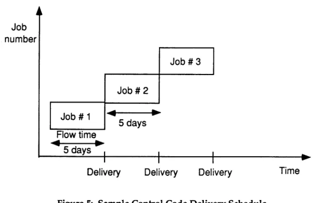
control code working on two jobs for ten days each. The control code will complete work on a job every five days (see Figure 4).

Job number Job # 3 Job # 2 Job # 1 . 1 5 days 4- -Flow time -a 10 days

Figure 4: Sample Control Code Schedule

Now, because of improved worker productivity, suppose that the labor input per job has decreased from eight hundred labor hours per job for unit number one to eighty labor hours per job for unit number 256. How do we plan the production of unit number 256?

8

Using optimal crew size to minimize labor required per job.

9

Assuming single shift operation.

1 0

There are ten workers per tool position. Since there are two tooling positions, the control code has twenty workers.

(27)

I'

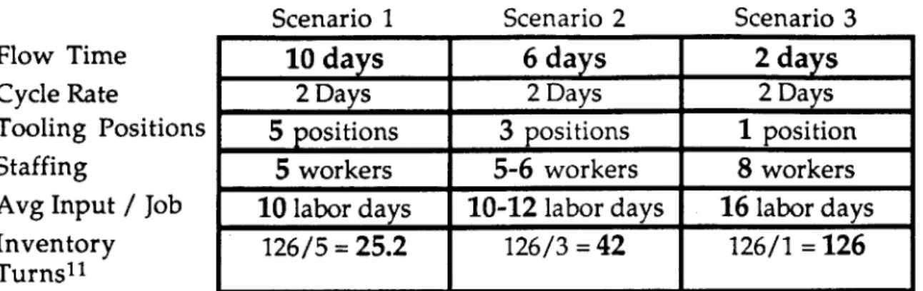
For unit 256, we see that one possible scenario is keep the number of flow days at ten and to decrease the control code head count from twenty to (2

* (80 hours / (ten days * 8 hours per worker-day) ) ) = 2 workers. With this scenario, the number of tools required remains at two. Alternately, we can decide to operate with five flow days in the control code and reduce the number of workers to (80 hours / (5 days * 8 hours per worker-day) ) = 2 workers (see Figure 5). Notice that even though the number of workers remain the same, the number of tools required at the control code decreases from two to one. As we will see later, these two different scenarios have significant implications on total product cost.

Job number Job # 3 Job # 2 Job # 1 _5dy

5 days

Flow time 5 days

(28)

2.3 Organizational Impact on Production Planning

In the above example, we see that by using available planning tools

differently, the production planning group can propose drastically different production plans that are responsive to management focus on labor

productivity and schedule adherence. However, as we will show in the next chapter, maximizing labor productivity alone by staying at optimal crew (and the flow time implied by the optimal crew size) can actually decrease

corporate profitability because of flow time cost.

2.4 Conclusion

As we see in this chapter, the process of planning and coordinating a complex production process such in an airplane manufacturing plant requires

extensive knowledge, experience, and coordination. In this chapter, I have outlined and described only some of the many different tools that Boeing's Industrial Engineering group uses to plan and coordinate this complex production process. In the next few chapters, we will see how lack of flow time cost visibility results in production plans that emphasized reduction of worker head count and preservation of manufacturing flow time. I show that these production plans, while successful in minimizing worker head count and assuring schedule adherence, sometimes resulted in longer process flow times and decreased corporate profitability.

(29)

FLOW TIME COST

3.1 Introduction

In Boeing's management accounting system, there is presently no visibility of

flow time cost. In this chapter, I present the motivation for understanding

flow time cost and detail three primary components of this cost: 1) inventory carrying cost, 2) revenue opportunity cost, and 3) variable tooling cost. Next, I discuss how the lack of flow time cost visibility causes the present production planning methodology to over emphasize head count reduction at the

expense of flow time and detail how these decisions adversely affect operational profitability. I then propose a near term flow time reduction strategy to reverse the effects of these decisions. Finally, I recommend that flow time cost be incorporated into the production planning methodology.

3.2 Motivation

Within Boeing management, adherence to schedule is considered

paramount. This is partly due to the significant cost penalties involved when airplane deliveries are delayed. The sequential nature of the manufacturing process work flow dictates that upon completion of each production cycle, each job in the production line must advance to the next control code in the manufacturing sequence. This is because the delay of a single job within the sequential manufacturing process could disrupt the work flow on the

production line and postpone the delivery of every successive airplane by the Chapter 3

(30)

length of the delay. Presently, if a job is not completed within the allotted flow time, the incomplete job is nevertheless moved on to the next control code so that all following airplanes in the production line can proceed to their next respective control codes. The offending late airplane will then have two separate crews working on it during the manufacturing flow time in the next control code. One of the teams working on the airplane will be the regular crew of the new control code, the other is a special crew from the previous control code sent over to complete all remaining incomplete tasks from the previous control code. These incomplete jobs, called "travellers", are

monitored very closely by manufacturing management. Thus, the prevailing attitude within manufacturing is to protect schedule jealously because of the huge cost involved. This philosophy has resulted in manufacturing practices which emphasize "Just-in-case" instead of "Just-in-time". One of the results of these practices is the lengthy flow time present in the current

manufacturing process.

Manufacturing Flow Time Cost Visibility

In Boeing's management accounting system, there is little recognition of cost associated with manufacturing flow time. The lack of flow time cost

visibility, coupled with the importance of completing jobs to schedule (while maintaining the capability to manage unforeseen disruptions) and close management scrutiny on work force head count, all contribute to the present practice of reducing work force head count while preserving manufacturing flow time. Consequently, as the total labor required to perform pre-assigned manufacturing tasks within a control code decreases because of worker

(31)

learning, current production planning methodology relies heavily on worker head count reductions to realize learning curve benefits, while at the same time preserving manufacturing flow time in order to insure that control codes can adhere to tight production schedules and be protected against unforesleen disruptions.

This methodology, which does not fully take flow time cost into

account during the production planning process (see section 3.3 for discussion on components of flow time cost), actually increases manufacturing cost significantly when applied within a high capital, high inventory

environment such as Boeing's final assembly process. In this thesis, I propose an alternate production planning methodology, one which does take into account the cost of manufacturing flow time and still operates within the requirement of strict schedule adherence.

Specifically, I suggest that in most instances within the manufacturing environment, flow time buffering is not the only method available to protect against unforeseen disruptions. I suggest that in certain instances, increases in labor head count and/or capital investments are just as effective as flow time buffers in protecting against the effects of unforeseen disruptions. In the proposed methodology, we evaluate and compare production alternatives (such as increased labor head count and/or additional capital investments), which are comparably capable of protecting the production schedule from disruption, against the alternative of flow time buffering.

(32)

3.3 Flow Time Cost Elements

Given the definition of flow time in section 3.2, in this section I show that there are three significant elements of cost associated with manufacturing flow time. Specifically, I show that flow time cost is composed of three major cost elements: 1) inventory carrying cost, 2) revenue opportunity cost, and 3) variable tooling cost.

Inventory Carrying Cost

The first element of flow time cost is the opportunity cost of money associated with carrying the value of the work-in-process (WIP) inventory for the

duration of the control code flow time. I call this opportunity cost the

inventory carrying cost (recognizing that this cost is only a subset of the more general definition of inventory carrying cost which also includes the

opportunity cost of carrying raw materials and finished goods).

The inventory carrying cost arises as follows. By having money

invested in inventory, a company loses the use of its money for the duration of the manufacturing flow time. Since the minimum return of the

company's money is simple interest (such as bank CDs), each flow day the work-in-process (WIP) inventory is being worked on in the manufacturing process costs the company, at the very least, simple interest expense on the full value of the WIP inventory1_{. Because inventory carrying cost is a}

function of inventory value, this component of flow time cost varies with

1_{Inventory carrying rate should also include storage cost, insurance, spoilage and obsolescence,}

(33)

flow time as value is being added during each flow day of the manufacturing process (see figure 2).

Calculating Inventory Carrying Cost

Calculating inventory carrying cost for a manufacturing process requires detailed, precise information regarding cost-adding activities ongoing within the manufacturing process. Specifically, to calculate inventory carrying cost for each day within the manufacturing process, we must know the labor required to complete assigned tasks within each control code, the relative sequence of all control codes and the flow and costs of all parts and sub-systems into the manufacturing process. With this information, daily inventory carrying cost for each control code (and for each manufacturing day) can be easily calculated.

An example

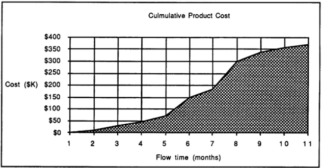
Given a cumulative product cost curve (or value-added curve) as shown in Figure 1, how do we calculate the product's inventory carrying cost

component of flow time cost?

We can calculate the inventory cost curve for this product for every flow day of the manufacturing process by making use of the formula below:

Inventory carrying cost for flow day t= WIP inventory at flow day t *

inventory carrying rate

(34)

or, in simplified notation:

ICC (flow day t)= WIP (flow day t) * ICR (Equation 3.1)

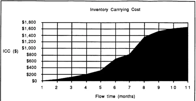
Applying this equation for every point on the cumulative product cost curve2_{, we get the inventory carrying cost profile as shown in Figure 2. Not} surprisingly, we see that the inventory carrying cost curve has the identical shape as the cumulative product cost curve since the inventory carrying cost for a particular flow day is simply the cumulative product cost for that flow day multiplied by the inventory carrying rate. Note that Figure 2 is calculated in terms of inventory carrying cost per plane.

Culmulative Product Cost $400 $350 $300 $250 Cost ($K) $200 $150 $100 $50 $0 .,o 1 2 3 4 5 6 7 8 9 10 11

Flow time (months)

Figure 1: Cumulative Product Cost Curve

2

(35)

Inventory Carrrying Cost $1,800 $1,600 $1,400 $1,200 ICC (s) $1'000 $800 $600 $400 $200 $0 $1,600

I

2 3 4 5 6 7 8 9 10 11

Flow time (months)

Figure 2: Inventory Carrying Cost ($/Airplane)

Revenue Opportunity Cost

In a market where there is immediate substantial demand for a company's product, there is a second element of cost associated with manufacturing flow time called revenue opportunity cost. Revenue opportunity cost is the

potential revenue opportunity associated with collecting incoming sales revenue earlier if a shorter product flow time can be realized (deliver earlier). For example, in the airplane industry, demand for airplanes currently far exceeds supply. Boeing commercial airplane group currently has an $85 billion, four year order backlog3. An airline ordering a Boeing 747-400 today will not get delivery of the airplane until approximately 19974. Given current

1

3_{Boeing News.} 4_{Boeing News.}

(36)

'-I

market conditions5_{, with airline passenger traffic predicted to grow at over 4%}

annually for the next decade6_{, airline customers are eager to take delivery of}

newly designed, fuel efficient airplanes as quickly as possible. Given this market environment, there are significant revenue opportunity benefits associated with shorter product flow time (and earlier product delivery).

Flow Through vs. Flow Back

Before we calculate the revenue opportunity benefit of shorter flow time, let us first discuss two possible implementations of flow time reduction.

Imagine that a control code within the manufacturing process which

presently has eight days of flow time (operating at a four day production rate) reduced its flow time by one day. Implemented in isolation, the one day flow time reduction at the control code brings about no tangible benefits to the operation. This is because the one day flow time reduction, implemented in isolation, has simply created a one day buffer inventory at the particular control code. To realize the benefits of flow time reduction, the inventory buffer must be either "flow through" or "flow back" the manufacturing process.

By "flow through", we mean that the one day reduction is pushed through all the subsequent control codes in the manufacturing process. To accomplish this, all the control codes following the present control code must

5

This chapter was written prior to the 1991 Iraq-Kuwait crisis, which has had significant short term impact on airline operations and profitability due to increasing oil prices (up to 30% price increases in jet fuel prices) and decreasing passenger traffic (because of terrorist threats). The long term effects of the crisis on airline operations is not clear.

(37)

compress their schedule (by the amount of the flow time reduction) on the very first airplane when the flow through is to occur. Note that the

compression for all subsequent control codes occurs only for the very first airplane during the flow through process. Thereafter, the schedules for all subsequent control codes are thereby advanced by one day. However, since there are no changes in either the flow time nor the production cycle time for these control codes, all these control codes would simply experience a one day compression for the first airplane when the flow time reduction is flowed through; after that, the control codes should continue to operate as normal, one day ahead of the schedule it would be following under the previous, longer flow time.

Flow Through Illustration

To illustrate, let us look at Figure three below. Figure three is a sample

production schedule for a hypothetical sequential job shop I have constructed to illustrate how flow time reductions can be flowed through the

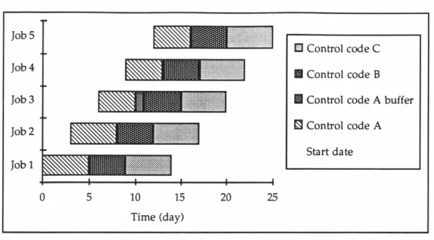
manufacturing process. From the figure, we see that the manufacturing process consists of three sequential control codes, control codes A, B, and C. We see that the manufacturing flow time for control codes A, B, and C are five days, four days, and five days, respectively. From the schedule, we learn that the production line is operating at a three day production rate (a product is completed every three days). Note that for the first two jobs in the

production schedule, a new job is started and a completed job is shipped out every three days. Assume that during a flow time reduction effort, the work team at control code A found a one day flow time buffer that it can reduce

(38)

from its present flow time. How do we flow through this one day flow time reduction?

Table 1 below lists the start and completion dates for each of the control codes for all five jobs. Note that on job number four, where the flow time buffer is actually taken out of control code A and flow through the

manufacturing process, control codes B and C had to accelerate their

production schedules to "flow through" the flow time reduction (the dates in parenthesis listed in Table 1 are the pre-accelerated start and completion dates for each control code under the previous, longer flow time). We see from both Figure 3 and Table 1 that after the one time schedule acceleration to flow through the flow time reduction, control codes B and C settle back to their regular production pace, starting and completing each job after the first flowed through job (job number four in the example) one day ahead of the old schedule. Note that this analysis applies similarly to a more complicated manufacturing process involving parallel flow of sequential manufacturing processes. The only difference occurs when the control code where flow time is reduced is positioned before the integration point (where the parallel

processes converge). In this case, all parts in the parallel process flow that will be integrated into the first flowed through job will also need to have their schedules accelerated in order to synchronize arrival time at the process integration point.

(39)

QNz...

-IziIs

0 5 10 15

Time (day)

20 25

Figure 3: Production Schedule to Illustrate "Flow Through" Concept

Control Code A Control Code B Control Code C Start Date Cmpletn Start Date Cmpletn Start Date Cmpletn

Date Date Date

0 4 5 8 9 13

3 7 8 11 12 16

6 10 11 14 15 19

9 12(13) 13(14) 16(17) 17(18) 21(22)

12 15 16 19 20 24

Table 1: Start and Completion Dates for Five Jobs in Production Schedule

Advantages and Disadvantages of Flow Through versus Flow Back Instead of flow through, the company can choose to "flow back" the inventory buffer of the flow time reduction. That is, given the flow time reduction, all upstream control codes can start one day later than the old schedule and still be able to meet current delivery schedule. Since flow back

Job 5 Job 4 Job 3 Job 2 Job1 O Control code C M Control code B * Control code A buffer 0 Control code A Start date Job 1 Job 2 Job 3 Job 4 Job 5 5 . -- I

(40)

I-rn

-simply requires that upstream control codes start later, there is no

compression of the schedule and implementation is far easier than flow through. However, since flow through shifts the production schedule ahead

by the length of the flow time reduction, flow through achieves revenue

opportunity cost savings as well as inventory carrying cost savings (for a manufacturing process involving parallel processes, revenue opportunity costs savings can only be achieved if the flow time reduction is for a control code on the critical path of the manufacturing process). On the other hand, flow back simply takes advantage of the flow time reduction by pushing back the starting date of the production schedule, thus helping the company only to reduce inventory carrying cost and not realize any revenue opportunity cost savings.

To summarize, a company can choose to either flow through or flow back flow time reductions. By choosing to flow through flow time reductions, a company will have to accelerate the production schedule for a pre-selected

job in order to flow the flow time buffer through the manufacturing process.

Once accomplished, all control codes (except the control code where the flow time reduction took place) in the manufacturing process will operate with the same flow time at the same production rate. The only noticeable difference will be that the production schedule will be shifted forward by the length of the flow time reduction that is flowed through the manufacturing process.

By flowing through flow time reductions, a company will have to plan

production carefully in order to account for the schedule compression for the first flowed through job. However, because flow through shifts the

production forward by the length of the flow time reduction, flow through allows the company to realize revenue opportunity cost savings as well as

(41)

F'

inventory carrying cost reductions. Flow back, because it only involves delaying the starting date of every job after a designated flow back job, is very simple to implement. However, because flow back utilizes the flow time reduction by delaying the start dates, there are only inventory carrying cost savings and no revenue opportunity cost reductions. Put in other terms, a company can choose to implement the flow time reduction by either delivering earlier (flow through) or starting later (flow back).

Calculating Revenue Opportunity Cost

Calculating revenue opportunity cost for an airplane program requires knowledge of present production cycle rate, selling price of the aircraft,

customer pre-payment factor (if applicable), and relevant interest rates. Note that revenue opportunity cost (benefits) only exist on control codes which are on the critical path of the manufacturing sequence. That is, in order to

improve the revenue opportunity element of flow time cost, the flow time for the entire product must be reduced and the income revenue stream brought forward (flow time reduction is flowed through the manufacturing process); thus, a reduction of the flow time for a control code that is not on the critical path of the manufacturing process does not reduce the product flow time and will not improve the revenue opportunity benefit of the product. Also, as previously noted, flow time reductions that are flowed back the manufacturing process will only bring about inventory carrying cost savings but not revenue opportunity benefits.

(42)

An example

Assume that manufacturing flow time for a much demanded product is ten months. Further assume that the product sells for $100 each and that the factory is operating at full capacity and has a two year order backlog. Thus, when a customer orders this product, the customer would not get delivery of the product for at least two years. Now, suppose that the company is

considering a proposal to reduce its product flow time from ten months to nine months. What is the revenue opportunity benefit of this one month flow time reduction?

The revenue opportunity benefits7 _{of the flow time reduction can be} calculated as follows. If the company flows the flow time reduction through the manufacturing process, it would be able to ship product to each of its customers a month earlier. This flow time reduction will therefore, from a cash flow standpoint, enable the company to collect its $100 revenue from each of its customers a month earlier than under the current, longer flow time. This shift in the revenue stream generates revenue opportunities for the company in the form of either simple interest or internal investments.

Variable Tooling Cost

Variable tooling cost is especially important in Boeing's high capital, labor intensive manufacturing environment. This element of flow time cost is associated with the cost of purchasing and servicing required production tools

7

The one month flow time reduction will also bring about inventory carrying cost savings (see section on inventory carrying cost).

(43)

U

and equipment within the control codes in the manufacturing sequence. As noted previously, the number of job or tooling positions required in a control code is determined by the quotient of the control code flow time divided by the maximum cycle time (plus one if the remainder of the division is non-zero). For example, if control code 123 (a hypothetical control code) has eight days of flow time and is operating on a four day production cycle, the number of tooling positions (and in-process jobs) in the control code is equal to 8/4 =

2. If, on the other hand, the production rate needs to be increased to a three day production cycle (a completed job from each control code every three days instead of every four days), a new tool would have to be purchased and

installed at the control code because the number of tooling positions required

by control code 123 to meet the requirements of the new three day production

environment is now (8/3 =2) +1 = 3 (we add one to the quotient because the

remainder of the division is non-zero).

Now, suppose that the control code flow time can be reduced to six days (we will discuss near term and far term flow time reduction strategies later in this thesis), then the tooling requirement for the control code would remain at two (6/3 = 2) and the additional tooling position would no longer be needed. Therefore, we see that significant tooling cost reductions can be achieved through control code flow time reduction.

Calculating Variable Tooling Cost

Calculating variable tooling cost for a control code requires an estimate of the incremental tooling cost, the planned maximum production cycle rate for the airplane program, and the projected control code flow time based on the

(44)

present production planning methodology. Note that variable tooling cost (and savings) occur in a step-wise manner (see Figure 4). This is because the incremental tooling cost being evaluated increases as steps (a function of the production cycle time). For instance, in the example above, a one day flow time reduction in control code 123 (bringing the control code flow time to seven days), is of no value within the variable tooling cost dimension8 _{since a} one day flow time reduction will not decrease the number of tools required at the control code (the number of tooling positions required at the control code is (7/3 = 2) + 1) = 3 positions.)

An example

To demonstrate a variable tooling cost calculation, we will use the control code above that is operating with eight days of flow time in a four cycle production cycle (a completed job every four days). Assume that because of market conditions, the factory wants to accelerate the production rate to a three day production cycle (a completed job every three days).

As we saw earlier, going from a four day production rate to a three day production rate will necessitate purchase and installation of a new tool since the number of tooling positions required by the control code will increase from 8/4 = 2 positions to 8/3 = 2 + 1= 3 positions. We will assume that the

incremental tooling cost is $1.2 million dollars. What is the variable tooling cost (benefit) for flow time reduction at this control code?

8_{The one day flow time reduction does bring about inventory carrying cost savings for the control}

(45)

In this example, if we do not reduce manufacturing flow time at the control code, we will need to purchase a new tool for $1.2 million in order to produce at the faster three day production rate. If, however, we can reduce manufacturing flow time at the control code, we may be able to produce at the faster production rate without purchasing a new tool, thereby realizing

significant variable tooling cost savings. To calculate the variable tooling cost (benefit) of flow time reduction, we note that a one day flow time reduction (bringing the control code flow time to seven days) will not reduce the need for the new tool since the number of tooling positions at the control code is still (7/3 = 2) + 1 = 3 positions. On the other hand, if we can reduce the flow

time at the control code by two days (bringing the control code flow time to six days), we see that we no longer need to purchase the additional tool in order to produce at the faster production rate since the number of tooling position required now is 6/3 =2 positions (we already have two tools in the control code since we are presently operating with eight flow days in a four day production cycle, thus the number of tooling positions presently at the control code is 8/4 = 2 tools). Since a one day flow time reduction brings about no variable tooling benefit, but a two day flow time reduction brings about $1.2 million in variable tooling saving, we see that the variable tooling cost curve looks like a step function (see Figure 4).

Analysis of variance impact on manufacturing flow time

Signature

Signature redacted

Signature redacted

Signature redacted

I

Sgnature

redacted

redacted

Signature redacted

JUN

2

1991

TABLE OF CONTENTS

INTRODUCTION

Chapter 2

NATURE OF AIRCRAFT MANUFACTURING

job

job

Job

number

Job #3

Job #1

das

--.

0

I

I

I

I

4 dayq

Icc

5

c

2

5 days

FLOW TIME COST

I

I

QNz...

-IziIs