MHD modeling and numerical simulation with finite volume-type methods. Application to fusion plasma

HAL Id: tel-01551701

https://tel.archives-ouvertes.fr/tel-01551701v2

HAL is a multi-disciplinary open access

archive for the deposit and dissemination of sci-entific research documents, whether they are pub-lished or not. The documents may come from teaching and research institutions in France or abroad, or from public or private research centers.

L’archive ouverte pluridisciplinaire HAL, est destinée au dépôt et à la diffusion de documents scientifiques de niveau recherche, publiés ou non, émanant des établissements d’enseignement et de recherche français ou étrangers, des laboratoires publics ou privés.

volume-type methods. Application to fusion plasma

Elise Estibals

To cite this version:

Elise Estibals. MHD modeling and numerical simulation with finite volume-type methods. Application to fusion plasma. General Mathematics [math.GM]. Université Côte d’Azur, 2017. English. �NNT : 2017AZUR4023�. �tel-01551701v2�

´

Ecole doctorale de Sciences Fondamentales et Appliqu´

ees

Unit´

e de recherche : Sciences

Th`

ese de doctorat

Pr´

esent´

ee en vue de l’obtention du

grade de docteur en Math´

ematiques

de

UNIVERSIT´

E C ˆ

OTE D’AZUR

par

´

Elise Estibals

Mod´

elisation MHD et Simulation

Num´

erique par des M´

ethodes Volumes

Finis. Application aux Plasmas de Fusion

MHD Modeling and Numerical Simulation with Finite Volume-type Methods. Application to Fusion Plasmas

Dirig´ee par Herv´e Guillard, Directeur de recherche, INRIA Sophia Antipolis et co-dirig´ee par Afeintou Sangam, Maˆıtre de conf´erence, LJAD Nice Soutenue le 2 mai 2017

Devant le jury compos´e de :

R´emi Abgrall Prof., Universit´e de Z¨urich Examinateur Christophe Berthon Prof., Lab. de Math. J. Leray, Nantes Rapporteur Herv´e Guillard DR INRIA, LJAD, Universit´e de Nice Directeur de th`ese Boniface Nkonga Prof., LJAD, Universit´e de Nice Examinateur

Afeintou Sangam MCF, LJAD, Universit´e de Nice Co-directeur de th`ese ´

Contents

List of Figures v

List of Tables xi

Introduction 1

I Nuclear fusion. . . 1

II Inertial Confinement Fusion . . . 2

III Magnetic Confinement Fusion . . . 4

IV Fusion modeling . . . 6

V Organization of the manuscript . . . 7

Introduction 9 I La fusion thermonucl´eaire contrˆol´ee. . . 9

II Fusion par Confinement Inertiel . . . 11

III La Fusion par Confinement Magn´etique . . . 12

IV Mod´elisation de la fusion . . . 15

V Organisation du manuscrit. . . 16

R´esum´e 19 1 Fluid models 25 I Plasma modeling . . . 25

I.1 Kinetic model . . . 25

I.2 Macroscopic quantities . . . 26

I.3 Collision operators . . . 26

I.4 Moment equations . . . 28

i Mass conservation equation . . . 28

ii Momentum equation. . . 28

iii Energy equation . . . 30

I.5 Maxwell equations . . . 30

I.6 Bi-fluid MHD equations . . . 31

II Bi-fluid MHD equations in quasi-neutral regime . . . 34

III Bi-temperature Euler model . . . 36

III.1 Derivation of the bi-temperature model . . . 37

III.2 The bi-temperature model for large β parameter . . . 41

III.3 Properties of the bi-temperature Euler model . . . 43

IV Mono-fluid MHD models . . . 45

IV.1 Non-dimensional bi-fluid MHD model . . . 45

IV.2 Resistive MHD model for small δ_e,i∗ and bounded Rm . . . 49

i Conservative system . . . 50

ii Properties of the ideal MHD model . . . 51

IV.4 Discussion on the assumptions leading to MHD models . . . 53

V Conclusions . . . 53

2 Finite volume method 55 I Generalities on finite volume method . . . 55

I.1 Principles of finite volume method . . . 55

I.2 2-D cell-centered finite volume on rectangular mesh . . . 56

I.3 2-D vertex-centered finite volume on a triangular mesh. . . 59

II Cell-centered approach for cylindrical coordinates . . . 61

II.1 Ideal MHD equations in cylindrical coordinates . . . 61

II.2 Cell-centered approach in a circular mesh . . . 63

III Vertex-centered approach for the toroidal geometry . . . 67

III.1 Cylindrical coordinates for toroidal problem and divergence form . . 67

III.2 Mesh design and adaptation to the finite volume method . . . 69

IV Conclusions . . . 74

3 Relaxation scheme for the bi-temperature Euler model 75 I Presentation of the scheme . . . 75

II Transport step . . . 76

II.1 Properties of the relaxed system . . . 76

II.2 Relaxation flux . . . 78

III Projection step . . . 80

IV Numerical tests . . . 81

IV.1 Shock tube . . . 81

IV.2 Implosion . . . 85

IV.3 Sedov injection in 2-D Cartesian geometry. . . 92

IV.4 Sedov injection in a poloidal plane of a torus with axisymmetry initialization . . . 94

IV.5 Triple point problem in a rectangular computational domain . . . . 97

IV.6 Triple point problem in a disc in 2-D Cartesian geometry . . . 103

IV.7 Triple point problem in the plane of a torus with axisymmetry ini-tialization . . . 106

IV.8 Triple point problem in 3-D toroidal geometry . . . 108

V Conclusions . . . 111

4 On Euler potential for MHD models 113 I Issues on the divergence-free constraint. . . 113

I.1 Vector potential A method . . . 113

I.2 Powell’s source term . . . 114

I.3 Generalized Lagrange Multiplier . . . 114

I.4 Contrained transport method . . . 115

II An alternate method for divergence-free problem . . . 116

III Numerical resolution of ideal MHD equations with Euler potential . . . 117

III.1 Presentation of the scheme . . . 117

III.2 Transport step . . . 117

i Rusanov flux . . . 118

ii HLL flux . . . 118

Contents

III.3 Projection step . . . 122

i Cartesian coordinates . . . 122

ii Issue for cylindrical coordinates . . . 123

IV Numerical resolution of resistive MHD equations . . . 123

IV.1 Presentation of the proposed scheme . . . 124

IV.2 Presentation of the resistive step . . . 124

IV.3 Resistive step in Cartesian coordinates . . . 125

i Order 2 . . . 125

ii Order 4 . . . 126

IV.4 Resistive step in cylindrical coordinates . . . 129

i Order 2 . . . 129

ii Order 4 . . . 131

V Numerical results . . . 133

V.1 Brio-Wu problem for ideal MHD . . . 133

V.2 Orszag-Tang problem for ideal MHD . . . 141

V.3 Kelvin-Helmholtz instabilities for ideal MHD . . . 145

V.4 Kelvin-Helmholtz instabilities for resistive MHD . . . 147

V.5 Screw pinch equilibrium with uniform density in cylindrical coordi-nates for ideal MHD . . . 150

V.6 Screw pinch equilibrium with uniform density in Cartesian coordi-nates for ideal MHD . . . 155

V.7 Screw pinch equilibrium with uniform density in Cartesian coordi-nates for resistive MHD . . . 157

VI Conclusions . . . 160

Conclusions 161

Conclusions 163

List of Figures

1 Fusion reaction [1]. . . 1

2 Direct drive of the laser beam to heat and compress the target [2]. . . 3

3 Indirect drive of the laser beam to heat and compress the target [3]. . . 3

4 Fast ignition for the direct drive method [4]. . . 4

5 Representation of a tokamak [5]. . . 5

6 Representation of the future ITER tokamak [6]. . . 6

1 La r´eaction de fusion [1]. . . 9

2 Attaque directe d’un laser pour chauffer et comprimer la cible [2].. . . 11

3 Attaque indirecte d’un laser pour chauffer et comprimer la cible [3]. . . 12

4 Allumage rapide pour l’attaque directe [4].. . . 12

5 Repr´esentation d’un tokamak [5]. . . 13

6 Repr´esentation du futur tokamak ITER [6]. . . 15

1.1 The four cases of Riemann problem for the bi-temperature Euler equa-tion: (a) 1-Rarefaction and 3-Shock, (b) 1-Shock and 3-Rarefaction, (c) 1-Rarefaction and 3-Rarefaction, (d) 1-Shock and 3-Shock.. . . 45

1.2 Riemann fan of the ideal MHD system. . . 52

2.1 Representation of a control cell Ωi,j in the cell-centered approach. . . 56

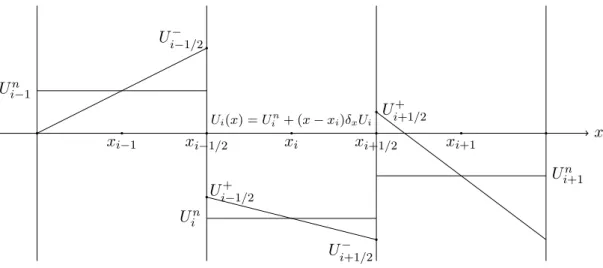
2.2 Piecewise linear reconstruction for the 1-D case.. . . 59

2.3 Representation of a control cell Ωi in the vertex-centered approach. . . 60

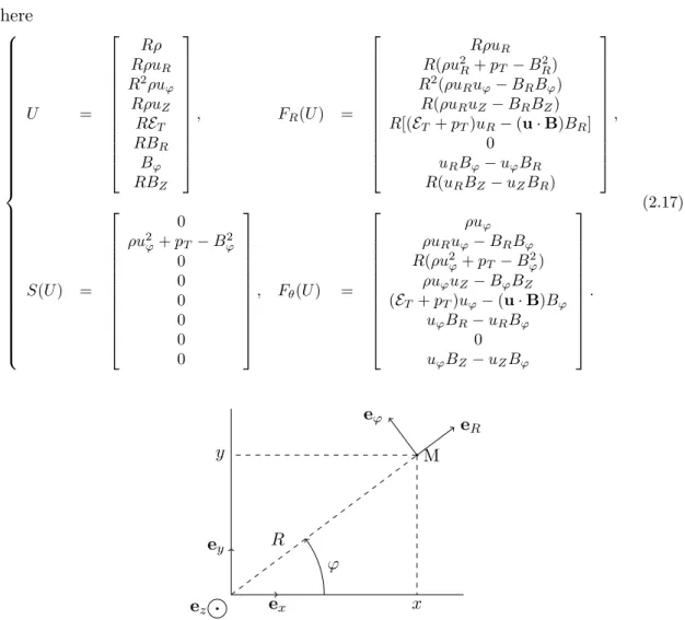
2.4 Cartesian and cylindrical basis representation. . . 63

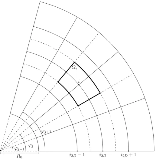
2.5 Representation of a cell Ωi,j in the cylindrical coordinates for the cell-centered approach. . . 67

2.6 Projection on eϕ of the Ωi cell control. . . 70

3.1 Riemann fan for the relaxed system (3.1). . . 80

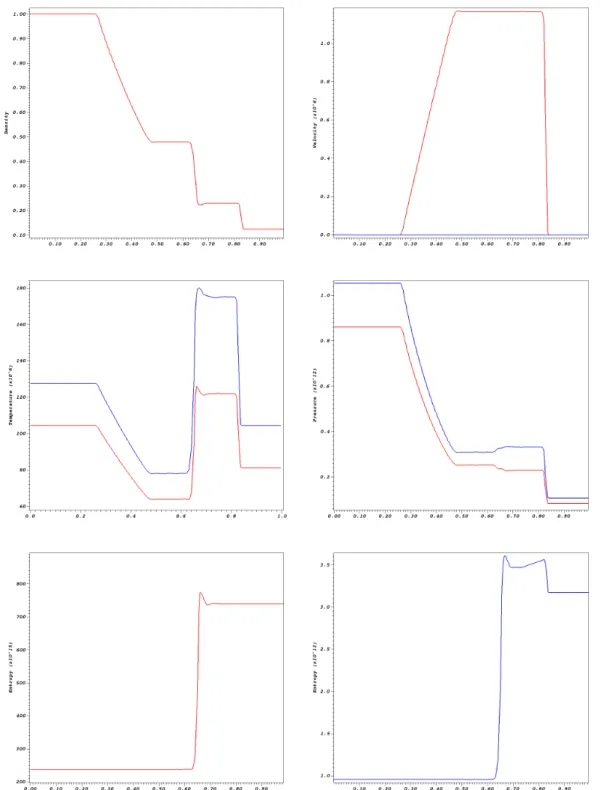
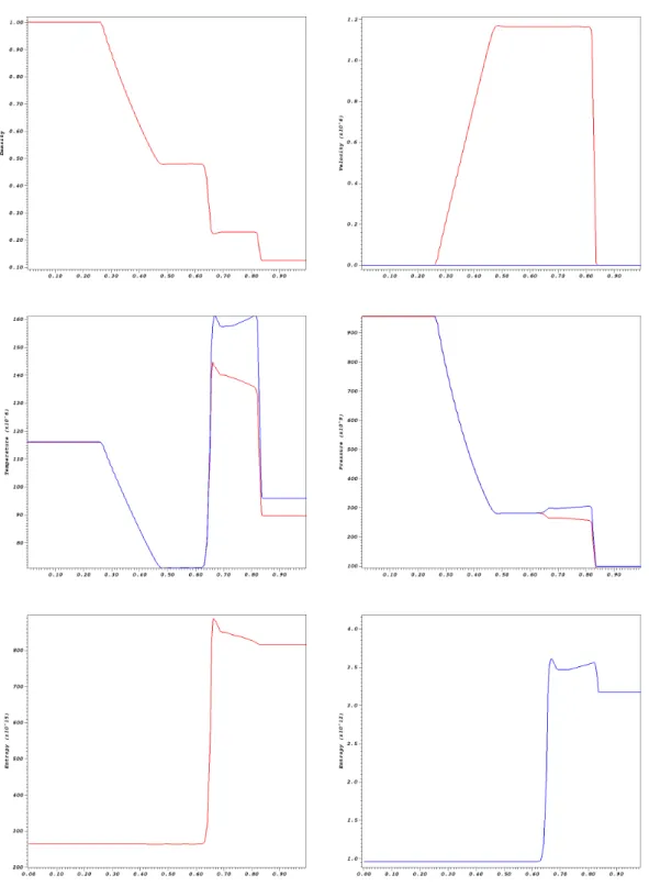
3.2 Shock tube problem at t = 8.6289 × 10−8s with νei = νie = 0. Solution at y = 0.5. Left-Top: Density, Right-Top: x-velocity in red, and y-velocity in blue, Left-Center: Electronic (red) and ionic (blue) temperatures, Right-Center: Electronic (red) and ionic(blue) pressures, Left-Bottom: Electronic entropy, Right-Bottom: Ionic entropy. . . 83

3.3 Shock tube problem at t = 8.6289 × 10−8s with νei 6= 0, νie 6= 0. Solution at y = 0.5. Left-Top: Density, Right-Top: x-velocity in red, and y-velocity in blue, Left-Center: Electronic (red) and ionic (blue) temperatures, Right-Center: Electronic (red) and ionic(blue) pressures, Left-Bottom: Electronic entropy, Right-Bottom: Ionic entropy. . . 84

3.4 Implosion problem, Similar mesh with 2145 points as the one used in nu-merical simulation. The mesh used in Section IV.2 has been obtained by a refinement of a factor 4 from the present one and contains 33153 (≈ 4 × 4 × 2145). . . 86

3.5 Implosion problem at t1 = 4.0901 × 10−7s. 2-D fields of Left-Top: Den-sity, Right-Top: Velocity, Left-Center: Electronic pressure, Right-Center: Ionic pressure, Left-Bottom: Electronic temperature, Right-Bottom: Ionic temperature. . . 87

3.6 Implosion problem at t1 = 4.0901 × 10−7s. 1-D fields at y = x of Left-Top: Density, Right-Left-Top: Radial (red) and tangential (blue) velocities, Left-Center: Electronic (red) and ionic (blue) temperatures, Right-Center: Electronic (red) and ionic (blue) pressures, Left-Bottom: Electronic en-tropy, Right-Bottom: Ionic entropy. . . 88

3.7 Implosion problem at t2 = 6.22 × 10−7s. 2-D fields of Left-Top: Density, Right-Top: Velocity, Left-Center: Electronic pressure, Right-Center: Ionic pressure, Left-Bottom: Electronic temperature, Right-Bottom: Ionic tem-perature. . . 89

3.8 Implosion problem at t2 = 6.22 × 10−7s. 1-D fields at y = x of Left-Top: Density, Right-Left-Top: Radial (red) and tangential (blue) velocities, Left-Center: Electronic (red) and ionic (blue) temperatures, Right-Center: Electronic (red) and ionic (blue) pressures, Left-Bottom: Electronic en-tropy, Right-Bottom: Ionic entropy. . . 90

3.9 Implosion problem, Density, Left: 1-D fields at y = x, Right: 2-D isolines at ρ = 1 (black), ρ = 1.585 (violet), ρ = 2.369 (blue), ρ = 4.259 (green), and ρ = 6.047 (red). Top: t1 = 4.0901 × 10−7s, Middle: t2= 6.22 × 10−7s, Bottom: t3= 8.4973 × 10−7s. . . 91 3.10 Sedov injection in 2-D Cartesian geometry at t = 9.7634 × 10−6s. Left:

Density, Center: Electronic pressure, Right: Ionic pressure. . . 93

3.11 Sedov injection in 2-D Cartesian geometry. 1-D profiles at Left: t = 6.73 × 10−10s, Middle: t = 6.73 × 10−9s, Right: t = 9.7634 × 10−6s, Top: Density. Bottom: Electronic (red) and Ionic (blue) temperatures. . . 93

3.12 Sedov injection in axisymmetric toroidal geometry at t = 9.7634 × 10−6s. Comparison of the 2-D axisymmetric and 3D computations. Left: 2-D run, Right: 3-D run, Top: Density, Center: Electronic pressure, Bottom: Ionic pressure. . . 95

3.13 Sedov injection in 3-D toroidal geometry, toroidal velocity uϕat t = 9.7634× 10−6s along Z = 0. . . 96

3.14 Initialization of the triple point problem in a rectangle. . . 98

3.15 Triple point problem total internal energy at t = 3.5 (left) and at t = 5.0 (right), Top: Results from [40] for mono-temperature Euler equations where the top of the domain is obtained with the Volume of Fluid method and the bottom of the domain with the concentration equations, Bottom: Relaxation scheme for bi-temperature Euler equations with νei= νie= 0. . 99 3.16 Triple point problem without thermal exchange, νei = νie = 0,

Ti− Te Te

2-D field at t = 3.5 (Left), and t = 5.0 (Right). . . 99

3.17 Triple point problem with νei = νie = 0 at t = 3.5 (Left), and t = 5 (Right). 2-D fields of Top: Density, Middle: Electronic temperature, Bottom: Ionic temperature. . . 100

List of Figures

3.18 Triple point in a rectangular domain at t = 3.5 (left) and t = 5.0 (right). Comparison between the temperature of the case νei 6= 0 and νie 6= 0 (Top) and the electronic (middle) and ionic (bottom) temperatures of the case

νei = νie= 0. . . 101

3.19 Triple point in a rectangular domain at t = 3.5 (left) and t = 5.0 (right). Comparison between the density of the case νei6= 0 and νie 6= 0 (Top) and the one of the case νei= νie= 0 (Bottom). . . 102

3.20 The three domain of the triple point problem in the (R, Z) plane.. . . 103

3.21 Triple point problem in Cartesian geometry. Ti− Te Te 2-D fields at t = 2.1 × 10−9s (left), t = 4.7 × 10−9s (middle), and t = 1.35 × 10−8s (right). . 104

3.22 Triple point problem in Cartesian geometry. Initial data (Left) and so-lution at t = 1.1574 × 10−5s (Right). Top: Density, Center: Electronic temperature, Bottom: Total pressure. . . 105

3.23 Triple point problem at t = 1.1574 × 10−5s. Comparison of the results obtained in Cartesian geometry and in a torus. Left: 2-D axisymmetric run, Right: 2-D Cartesian run. Top: Density, Center: Electronic temperature, Bottom: Total pressure. . . 107

3.24 Triple point problem at t = 1.1574 × 10−5s. Comparison of the results obtained in Cartesian geometry and in a torus. Velocity vectors with density contours. Left: 2-D axisymmetric run, Right: 2-D Cartesian run. . . 108

3.25 Triple point problem initial domain in 3-D toroidal geometry. Left: for the poloidal planes 1 to 3. Right: for the rest of the poloidal planes (4 to 20). 109 3.26 Triple point problem initialization. Top: Poloidal planes 1 to 3, Bottom: Poloidal planes 4 to 20. Left: Density, Center: Electronic temperature, Right: Total pressure. . . 109

3.27 Triple point problem in 3-D toroidal geometry. Density at t = 1.1574 × 10−5s. Top-Left: Plane 1, Top-Center: Plane 2, Top-Right: Plane 3, Bottom-Left: Plane 4, Bottom-Center: Plane 20, Bottom-Right: Plane 10. . . 110

3.28 Triple point problem in 3-D toroidal geometry. Electronic temperature at t = 1.1574 × 10−5s. Top-Left: Plane 1, Top-Center: Plane 2, Top-Right: Plane 3, Bottom-Left: Plane 4, Bottom-Center: Plane 20, Bottom-Right: Plane 10. . . 110

3.29 Triple point problem in 3-D toroidal geometry. Total pressure at t = 1.1574 × 10−5s. Top-Left: Plane 1, Top-Center: Plane 2, Top-Right: Plane 3, Bottom-Left: Plane 4, Bottom-Center: Plane 20, Bottom-Right: Plane 10. . . 111

4.1 Localization of the magnetic and electric fields for the contrained transport method. Source: [11]. . . 115

4.2 Riemann fan with one intermediate state. . . 118

4.3 Riemann fan with four intermediate states. . . 122

4.4 Representation of the ghost cells for a Cartesian mesh. . . 127

4.5 1-D Brio-Wu problem, Solution at t = 0.1, O(1) Rusanov flux with and without projection, Top-Left: Density, Top-Right: Pressure, Middle-Left: x-velocity, Middle-Right: y-velocity, Left: y-magnetic field, Bottom-Right: Euler potential. . . 135

4.6 1-D Brio-Wu problem, Solution at t = 0.1, O(1) HLL flux with and with-out projection, Top-Left: Density, Top-Right: Pressure, Middle-Left: x-velocity, Middle-Right: y-x-velocity, Left: y-magnetic field, Bottom-Right: Euler potential. . . 136

4.7 1-D Brio-Wu problem, Solution at t = 0.1, O(1) HLLD flux with and with-out projection, Top-Left: Density, Top-Right: Pressure, Middle-Left: x-velocity, Middle-Right: y-x-velocity, Left: y-magnetic field, Bottom-Right: Euler potential. . . 137

4.8 1-D Brio-Wu problem, Solution at t = 0.1, O(2) Rusanov flux with and without projection, Top-Left: Density, Top-Right: Pressure, Middle-Left: x-velocity, Middle-Right: y-velocity, Left: y-magnetic field, Bottom-Right: Euler potential. . . 138

4.9 1-D Brio-Wu problem, Solution at t = 0.1, O(2) HLL flux with and with-out projection, Top-Left: Density, Top-Right: Pressure, Middle-Left: x-velocity, Middle-Right: y-x-velocity, Left: y-magnetic field, Bottom-Right: Euler potential. . . 139

4.10 1-D Brio-Wu problem, Solution at t = 0.1, O(2) HLLD flux with and with-out projection, Top-Left: Density, Top-Right: Pressure, Middle-Left: x-velocity, Middle-Right: y-x-velocity, Left: y-magnetic field, Bottom-Right: Euler potential. . . 140

4.11 2-D Brio-Wu problem, Euler potential ψ at t = 0.1. HLLD flux with pro-jection, Left: Order 1 in time and space, Right: Order 2 in time and space.

. . . 141

4.12 Orszag-Tang problem, HLLD O(2), t = 0.5, Top: Density field, Bottom: Pressure field, Left: Scheme without projection, Right: Scheme with pro-jection. . . 143

4.13 Orszag-Tang problem, HLLD O(2), t = 0.5, Pressure along y = 0.3125, Red: Scheme without projection, Blue: Scheme with projection. . . 143

4.14 Orszag-Tang problem, HLLD O(2), Top-Left: ∇ · B field at t = 0.5 scheme without projection, Top-Right: ∇·B field at t = 0.5 scheme with projection, Bottom-Left: k∇ · BkL2(t), Bottom-Right: k∇ · Bk_∞(t), . . . 144

4.15 Orszag-Tang problem, HLLD O(2) with projection, t = 1.0, Left: Density field, Right: Pressure field. . . 144

4.16 Kelvin-Helmholtz instabilities for ideal MHD, Ratio Bpol Btor

, 256 × 512 mesh, O(2) HLLD flux. Column 1: t = 5.0, Column 2: t = 8.0, Column 3: t = 12.0, Column 4: t = 20.0. . . 146

4.17 Kelvin-Helmholtz instabilities for ideal MHD, 256 × 512 mesh, O(2) HLLD flux. Left: ||∇ · B||L2||(t), Right: ||∇ · B||∞(t). . . 146 4.18 Kelvin-Helmholtz instabilities for ideal MHD, Ratio Bpol

Btor

, O(2) HLLD flux with projection. Column 1: t = 5.0, Column 2: t = 8.0, Column 3: t = 12.0, Column 4: t = 20.0. . . 147

4.19 Kelvin-Helmholtz instabilities for resistive MHD, η = 5 × 10−4, Ratio Bpol Btor , HLLD O(2), Top: Order 2 for the resistive step, Bottom: Order 4 for the resistive step, Column 1: t = 5.0, Column 2: t = 8.0, Column 3: t = 12.0, Column 4: t = 20.0. . . 148

List of Figures

4.20 Kelvin-Helmholtz instabilities for resistive MHD, η = 10−3, Ratio Bpol Btor , HLLD O(2), Top: Order 2 for the resistive step, Bottom: Order 4 for the resistive step, Column 1: t = 5.0, Column 2: t = 8.0, Column 3: t = 12.0, Column 4: t = 20.0. . . 149

4.21 Screw pinch equilibrium: Exact solution. Left: Pressure, Right: ϕ-magnetic field. . . 151

4.22 Screw pinch equilibrium in cylindrical coordinates, All R. Rusanov O(1). Left: Pressure, Right: Bϕ. . . 151 4.23 Screw pinch equilibrium in cylindrical coordinates, All R. HLL O(1). Left:

Pressure, Right: Bϕ. . . 152 4.24 Screw pinch equilibrium in cylindrical coordinates, All R. HLLD O(1).

Left: Pressure, Right: Bϕ. . . 152 4.25 Screw pinch equilibrium in cylindrical coordinates. First order in time and

space. Comparison of the scheme with projection and of the one without projection. Left: Rusanov flux, Right: HLL flux. . . 152

4.26 Screw pinch equilibrium in cylindrical coordinates. O(1) HLLD flux. Evo-lution of Left: the Residu in function time iteration. Right: Relative error of Bϕ in function of time. . . 153 4.27 Screw pinch equilibrium in cylindrical coordinates, All R. Rusanov O(2).

Left: Pressure, Right: Bϕ. . . 153 4.28 Screw pinch equilibrium in cylindrical coordinates, All R. HLL O(2). Left:

Pressure, Right: Bϕ. . . 153 4.29 Screw pinch equilibrium in cylindrical coordinates, All R. HLLD O(2).

Left: Pressure, Right: Bϕ. . . 154 4.30 Screw pinch equilibrium in cylindrical coordinates. Second order in time

and space. Comparison of the scheme with projection and of the one with-out projection. Left: Rusanov flux, Right: HLL flux. . . 154

4.31 Screw pinch equilibrium in cylindrical coordinates. O(2) HLLD flux. Evo-lution of Left: the Residu in function time iteration. Right: Relative error of Bϕ in function of time. . . 154 4.32 Screw pinch in Cartesian geometry. Comparison of the HLLD scheme with

and without projection at the second order in time and space. Relative error of the pressure in function of Alfv´en time. . . 156

4.33 Screw pinch equilibrium in Cartesian geometry for ideal MHD. Comparison of the HLLD schemes with and without projection. Final pressure field, Left: Scheme with projection, Right: Scheme without projection. . . 156

4.34 Screw pinch in Cartesian geometry for resistive MHD with η = 1.0 × 10−6. Comparison of the HLLD scheme with and without projection at the second order in time and space. Relative error of the pressure in function of Alfv´en time. Left: Resistive step at the second order, Right: Resistive step at the fourth order. . . 158

4.35 Screw pinch equilibrium in Cartesian geometry for resistive MHD. η = 1.0 × 10−6. Comparison of the HLLD schemes with and without projection. Final pressure field, Left: Scheme with projection, Right: Scheme without projection. Top: Resistive step at the second order, Bottom: Resistive step at the fourth order. . . 159

List of Tables

1 Confinement parameters in ICF and MCF. . . 2

2 Param`etres de confinement de la FCI et de la FCM. . . 10

1.1 Value of the inertial lengths and resistivity for the tokamak Iter at the center, and at the edge of the plasma. . . 53

3.1 Initial data for the shock tube problem. . . 81

3.2 Initial data for the implosion problem. . . 86

3.3 Initial data of the three states of the triple points problem. . . 103

4.1 Initial data of Brio-Wu problem. . . 134

4.2 Initial data of Orszag-Tang 2-D problem. . . 142

4.3 Initial data of Kelvin-Helmholtz instabilities. . . 145

Introduction

The question of energy remains important and central for human being. Energy enters greatly in all domains of human activities: food production, home heat and light, indus-trial facility operations, public and private transportation demands, communication needs, state safety requirement. The standard of living and energy consumption are intimately linked so that the quality of life is correlated with a reasonable price of consumed energy. The increasing demand of energy, the very limited energy resource accessibility by the world will probably become worse in the next future. This situation is intensified by environment requirements imposed to the portfolio energy resources available. Energy sources having reduced greenhouse gases, limited waste disposal, cheap cost production are then investigated to alleviate the world energy situation. Among world existing energy source options [37]: coal, oil, natural gas, wind energy, solar power, hydroelectricity, and nuclear fission energy, nuclear fusion power potentially fulfills the above standards.

I

Nuclear fusion

Fusion is the thermonuclear reaction that consists of merging two light atoms to produce a heavy one, and fast neutrons carrying a lot of energy as shown in Figure1.

Figure 1: Fusion reaction [1].

Fusion is the process which powers the sun and the stars. In future fusion reactors envisaged on Earth, energy will be released by gathering together hydrogen isotopes, namely deuterium and tritium. These fuels are virtually unlimited. Deuterium is abundant in ocean water. There is 1 atom of deuterium for every 6700 atoms of hydrogen [37]. It will take 2 billions years to exhaust all the deuterium to operate fusion if we keep the present rate of world energy consumption. Deuterium can be easily extracted from ocean water at very low coast. Conversely, there is no natural tritium, it can be generated by lithium reacting with neutrons directly in fusion reactor. Lithium is relatively abundant

on Earth and resources are estimated to be sufficient for 20000 years at the current world energy consumption. Nevertheless, this fusion reaction has two inconveniences: tritium is a radioactive element and lithium is a harmful substance. However, according to fission reactors, these situations are relatively minor, given that the half-life of tritium is 12.5 years compared with 2.4 × 107 years for uranium 236, 7.13 × 108 years for uranium 235, 4.5 × 109 _{years for uranium 236, 24000 years for plutonium 238, and still 6600 years for}

plutonium 240 [65].

Moreover, no greenhouse emissions, no other poisonous chemical materials are emitted into atmosphere by fusion reactions. Only the harmless inert gas helium is a product of the fusion reaction. Therefore, fusion reaction is attractive with respect to environment.

Fusion energy is thus a sustainable power source with favorable economic, environ-mental and safety attributes. Fusion occurs naturally at the extremely high pressures and temperatures which exist at the center of the sun, 15 millions of degrees Celsius. At the high temperatures experienced in the sun, any gas becomes a plasma, a mixture of negatively charged electrons and either positively charged atomic nuclei or ions. In order to reproduce fusion on earth, gases need to be heated to extremely high temperatures whereby atoms become completely ionized yielding a hot plasma. In fact, the amount of energy released and the number of thermonuclear fusion reactions in the volume of plasma depend on the density of particles and their temperature. The reaction gain be-comes higher than one when the energy released by fusion reactions is larger than the one invested in the plasma heating and confinement. This is formulated in the Lawson crite-rion relating the density n, temperature of the plasma and its confinement time τ [52]. For deuterium-tritium plasma heated to the temperature of 10 keV or 108K, this criterion reads:

nτ > 1020m−3s.

This condition can be fulfilled in different ways. A tremendous mass insures through gravitation forces a very large confinement time in stars. The confinement time is the lead-ing factor of fusion achievement. On earth two methods are currently actively studied, both experimentally, theoretically and numerically, to attain a large gain in fusion reac-tions: Inertial Fusion Confinement, abbreviated ICF, and Magnetic Fusion Confinement, known briefly as MCF. ICF leads to confine the plasma at extremely high density for a short time whereas MCF yields to achieve low densities for the relatively long times of several seconds. Comparison of the confinement times and densities in the two approaches is given in Table 1. The two ways are the matter of the next two sections.

ICF MCF

Particle density n in cm−3 1026 1014 Confinement time τ in s 10−11 10 Lawson criterion n τ in s cm−3 1015 1015

Table 1: Confinement parameters in ICF and MCF.

II

Inertial Confinement Fusion

Inertial Confinement Fusion relies exclusively on mass inertia to hold a fusion plasma in a small spherical volume for a short time corresponding to the time a sound wave needs to propagate from the surface to the center [8, 65]. Put simply, during this short time, the small volume of fuel is bringing to very high density, roughly about thousand times its solid

II. Inertial Confinement Fusion

density or liquid density, and high temperature by short energetic laser or ion beam pulses. Two principal schemes of interest are nowadays investigated to achieve ICF. The former, known as ablative implosive scheme, based on the action-reaction principle, consists in the irradiation of deuterium-tritium spherical shell by the use of powerful laser beam neatly set to obtain a symmetric illumination. Under the effect of the laser irradiation, the outer part of the spherical shell is vaporized, yielding a coronal plasma, which in turn expands towards the exterior: this is the so-called ablative process. By action-reaction principle, the coronal plasma expansion pushes the internal part of the shell toward the center in form of compressible waves. As the imploding material stagnates in the center, its kinetic energy is converted into internal energy. At this instant, the fuel consists of a highly compressed shell enclosing a hot spot of igniting fuel in the target center. A thermonuclear burn starts from the hot spot, travels radially from the target center to the periphery in the form of a wave, igniting then the whole fuel, which afterwards explodes. This process constitutes the direct-drive ICF illustrated in Figure2.

Figure 2: Direct drive of the laser beam to heat and compress the target [2]. An important problem in the implementation of direct-drive approach is the attain-ment of a high irradiation symmetry and accordingly the symmetry of dynamic plasma compression. In fact, a dissymetric irradiation of the target could be a seed of Rayleigh-Taylor-type instabilities that would hinder the efficiency of the fusion operation. To over-come this situation, another ablative implosive-type approach, known as indirect-drive, process has been developed and shown in Figure3. It consists in irradiation of cylindrical metallic cavity, made of gold or high-Z materials, of few millimeters in diameter and one centimeter long, the so-called hohlraum, from inside by using many intense laser beams. The deposited energy in the hohlraum is transformed in X-rays and generates then a isotropic and uniform illumination of the target inside the cavity [8,56,65].

Figure 3: Indirect drive of the laser beam to heat and compress the target [3]. Two largest facilities have been constructed to access conditions for ICF: National Ignition Facility (NIF) at Livermore in California in USA [47], and Laser M´egajoule (LMJ) at Barp near Bordeaux in France [16]. The NIF is operational since 2009.

In ablative scheme, the compression and ignition of the fuel are both dependent phases, and own contradictory conditions to fulfill at the same time. In order to cope this situation, the fast ignition concept has been developed [8, 56, 65]. The idea is to separate the two phases. In particular, one starts by compressing the target by using either direct-drive or indirect-direct-drive, then launches a ultrahigh-power short-pulse laser [62] to burn the compressed fuel [72]. Figure4 shows this process for the direct-drive.

a. b. c. d.

Figure 4: Fast ignition for the direct drive method [4].

III

Magnetic Confinement Fusion

Since plasma particles have high temperature, a contact with a material vessel intended to contain them will cool the plasma, leading to a possible fail of fusion reactions. Because plasma particles are charged, their dynamics across magnetic field lines is bounded whereas they move freely along magnetic field lines. The contact of plasma particles with the vessel walls due to a transversal movement could be thus avoided while their escape from the vessel by their helical trajectories along the magnetic field lines would still be plausible. The idea of MCF approach is to confine the plasma particles in devices with appropriate magnetic field configuration. There is plentiful magnetic configurations to maintain a hot plasma in a bounded domain, depending on the magnetic coils arrangement. They can split into two classes. The first one, known as open-ended confinement, is based on straight disposition of the magnetic coils. Such as a scheme is unable itself to confine a plasma since magnetic field lines are not closed, the device is then equipped with a driver allowing to bring back inside in the machine possible charged particles arriving at its ends. Open-ended confinement machines are thus MCF trap devices. Magnetic trap mirror [64], field reversed configuration [37] are for instance open-ended confinement devices.

The second class aim at using closed magnetic field lines to hold the plasma in bounded domain, thus it is termed toroidal confinement. In this way, magnetic coils are arranged such that they produce a toroidal field. However, in such a configuration, the magnetic field strength decreases with radius, which yields a radial velocity component and a drift of the particles towards the outside. To confine the plasma for a relatively long time, the field lines have to be twisted in such a manner as to lead to an absence of any radial field component. Stellarator, spheromak, reversed field pinch, levitated dipole, are examples of toroidal confinement devices [37].

Tokamak, a toroidal confinement machine, is the major device for MCF approach [19,

38,50, 79]. The main principal magnetic field is the toroidal field, which is produced by current external coils as illustrated in Figure 5. Tokamak approach also exploits largely the fact that the plasma is held inside the device by a balance of the magnetic field force and the gradient of the plasma pressure. As a consequence of this equilibrium, a poloidal component of magnetic field is immediately required for the magnetic force. In a tokamak, the poloidal field is principally generated by the plasma current, this current flowing in the toroidal direction. These currents and fields are shown in Figure 5.

III. Magnetic Confinement Fusion

Figure 5: Representation of a tokamak [5].

Moreover, the above equilibrium implies that the plasma pressure p is constrained to be not larger than a certain amount βmax of the magnetic energy B2/2µ0, where the

plasma β-parameter is given by:

β = p B2 2µ0

.

Creating strong magnetic field is technically challenging and cost-intensive, leading to the β-parameter to be not too small. As matter of fact, finding confinement configurations with β of a few percent constitutes current active research in MCF.

Controlled nuclear fusion reaction is expected to operate in a tokamak as follows. A mixture of deuterium and tritium is injected into the vacuum vessel contained in the tokamak. The mixture is heated externally until ignition is reached. There is three heating mechanisms: ohmic heating through the plasma resistivity, heating by high-frequency waves, heating by injection of beams of neutral particles. The two latter mechanisms could be used at any time of the heating phase whereas the former one is only used in the initial heating phase of the plasma, and then one of the two latter must take the relay. At the same time of heating phase, the magnetic field is generated by passing an electric current through coils wound around the torus. The plasma current produces a poloidal magnetic field and the two fields combine to produce a magnetic field as displayed in Figure 5. As soon as the plasma is heated to sufficiently high temperatures, it will be ignite yielding α-particles and neutrons. The α-particles are stopped in the plasma, provide additional plasma heating while the fusion mechanism continues running, whereas the neutrons penetrate the blanket of absorbing material surrounding the torus. If the confinement were ideal, the fusion operation could go until all fuel is used up.

as the stability requirement of the device [19,38,79], plasma heating, transport including turbulence and various types of instabilities [37, 38, 79], and technological issues as the design of coils supplying adequate magnetic fields.

Nevertheless, the quest of fusion energy with tokamak approach receives a great credit to go forward in this way. The International Thermonuclear Experimental Reac-tor, known as ITER, currently being built in Cadarache, France, is the largest tokamak dedicated to fusion energy, as shown in Figure 6. The roles of the ITER facility are to investigate burning plasma physics in long pulse, high-temperature, deuterium-tritium ex-periment, and address and solve a number of fusion technology issues that will arrive in a fusion reactor. The beginning of its operational phase is scheduled for 2025-2030 and the construction of the demonstration fusion reactor DEMO [80] will follow if ITER is suc-cessful. Finally, the commercial fusion reactor PROTO will be constructed upon DEMO results.

Figure 6: Representation of the future ITER tokamak [6].

IV

Fusion modeling

Issues on controlled thermonuclear fusion can be basically split into plasma physics and technological requirements.

Technological issues are dependent of the approach chosen to achieve fusion. ICF techno-logical demands roughly turned around high powerful laser, high-ion accelerators, targets. These issues are described in [8, 27, 65] and references there in. MCF technological requirements concern mainly the design of supraconductor coils magnets intended to gen-erate high-toroidal magnetic fields, of efficient heating sources. However, ICF and MCF schemes share the problem regarding material would be used to design the wall receiving energetic neutrons that escape from ICF target or that MCF device vessel vacuum.

Fusion plasma physics is concerned with the description of charged particle dynam-ics inside the considered device. There are three basdynam-ics approaches to plasma physdynam-ics: particle theory, kinetic theory, and hydrodynamic theory.

The particle theory is using equations of motion for individual plasma particles, and with the help simulation codes and appropriate averages the plasma physics is analyzed. This

V. Organization of the manuscript

approach is also called N-body model, where N is assumed to represent the number of plasma particles. As the fusion plasma owns very large number of particles, as quoted in previous Sections, the accuracy of the model will require a large N in order simulate the plasma. Despite the existence of codes dealing with N-body model, kinetic theory is favored with respect to the particle approach, N-body model becoming thus the base model of hierarchy ones to derive from it.

Kinetic theory is based on a set equations for distribution functions of the plasma particles that encodes their dynamics in time, physical and velocities space, together with Maxwell equations. Kinetic theories can accurately model such a system owning large number of particles. However, numerical computations of kinetic theories are, in general, resource consuming both in time and storage space, and are limited in a small computational do-main of physical/velocities space [44]. Large information yielded by kinetic models are not often accessible by experiment. Conversely fluid models constructed on velocity moments provide pertinent plasma parameters on a large time and a large domain [54, 55], which fit with experimental data.

In the either hydrodynamic or fluid models the conservation laws of mass, momentum and energy are coupled to Maxwell equations. One-fluid equations, two-fluid system, MHD equations [24, 9, 10,37,38,43, 42], two-temperature Euler system [26, 29,51,69,7, 32] are for instance fluid models.

Plasma modeling enables to study the plasma behavior which translates to three impor-tant types of transport theory: heat conduction, particles diffusion, and magnetic field diffusion. It infers that plasma modeling tackles the understanding and controlling of en-ergy confinement. Analyzing waves contained in systems brought by the modeling gives ways on choosing frequency waves that will heat the plasma.

V

Organization of the manuscript

This work is a combination of plasma physics modeling and numerical analysis. It is structured in four chapters and a conclusion. The first two deals with modeling whereas the last two concern numerical analysis. The content is the following.

Chapter1. In this chapter we recall the kinetic equation of a magnetized plasma and its corresponding fluid MHD equations. Then, using the non-dimensional scaling of the bi-fluid MHD equations, we give the assumptions leading to the bi-temperature Euler model and the ideal and resistive MHD ones. The proposed derivation of the bi-temperature Euler model is more general than the ones suggested in [26,37,43,51,7].

Chapter2. General principles of finite volume method are reviewed in this chapter, both for structured and non-structured tessellations aimed at approximating the three models derived previously. Having in the mind future applications to MCF in tokamak approach, we study the modification of finite volume type method to approximate the solutions of these models in a toroidal geometry. The scheme we proposed is based on recent works reported in [21, 18]. However, such as application is not straightforward due to both the complexity of the models and the unstructured tessellation used to adequately mesh the toroidal geometry of the torus.

Chapter 3. The numerical strategy set up in Chapter 2 uses a relaxation scheme to approximate the bi-temperature Euler model. In this chapter we give all steps leading to

the construction of this relaxation scheme. Numerical tests are also proposed to assess the performance of this scheme. This scheme has been accepted for publication [7].

Chapters1–3are gathered in [32] and published as internal report.

Chapter 4. The MHD equations coupled to the Maxwell’s equation which contains the divergence-free constraint of the magnetic field, has to be maintained by the numerical approximation. A strategy is designed ensuring that the magnetic field computed by stan-dard Finite volume approximation will be solenoidal, both for Cartesian and cylindrical coordinates. Various numerical tests on well-known standard problems in MHD in 2D-geometry are performed in different geometries in order to validate the proposed numerical method.

Conclusion. Finally, our conclusions are given in the last chapter. Forthcoming works are also proposed.

Introduction

La question de l’´energie reste importante et centrale pour l’humanit´e. L’´energie entre largement dans tous les grands domaines des activit´es humaines : la production de nourri-ture, le chauffage et l’´eclairage des habitations, les transports priv´es et publics, les usines industrielles de production, les communications, la s´ecurit´e de l’ ´Etat. Le niveau de vie et la consommation d’´energie sont intimement li´ees si bien que la qualit´e de vie est corr´el´ee `

a un prix raisonnable de l’´energie consomm´ee.

L’augmentation des besoins en ´energie ainsi la quantit´e tr`es limit´ee des ressources ´energ´etiques accessibles sur Terre s’empireront probablement dans les ann´ees `a venir. Cette situation est amplifi´ee par les normes environnementales exig´ees `a l’ensemble des ´energies disponibles. Les sources d’´energie `a moindre effet de serre et quantit´e de d´echets, et `a un coˆut de production relativement faible sont alors explor´ees. Parmi les diff´erentes sources d’´energie envisageables [37], le charbon, le p´etrole, le gaz naturel, l’´energie ´eolienne, l’´energie solaire, l’´energie hydro´electrique, ainsi que la fission nucl´eaire, la fusion ther-monucl´eaire contrˆol´ee satisferait les crit`eres pr´ec´edents.

I

La fusion thermonucl´

eaire contrˆ

ol´

ee

La fusion est une r´eaction thermonucl´eaire qui consiste `a mettre ensemble deux atomes l´egers pour obtenir un atome plus lourd et des neutrons rapides transportant une grande quantit´e d’´energie, comme le montre la figure1.

Figure 1: La r´eaction de fusion [1].

C’est de la r´eaction de fusion de leurs composants chimiques que le soleil et les ´etoiles s’auto-entretiennent. Dans les futurs r´eacteurs de fusion envisag´es sur Terre, l’´energie sera obtenue par la fusion de deux isotopes de l’hydrog`ene, le deuterium et le tritium. Les r´eserves de ces combustibles sont relativement illimit´ees. Le deuterium est tr`es abondant dans les oc´eans. Il y a un atome de deuterium pour 6700 atomes d’hydrog`ene [?]. Il faudrait plus de 2 millions d’ann´ees pour ´epuiser tout le deuterium n´ecessaire `a la fusion

si on garde le niveau actuel de consommation d’´energie. Le deuterium peut ˆetre extrait ais´ement de l’eau des oc´eans `a un coˆut minimum. Au contraire, le tritium n’existe pas naturellement sur Terre, il peut ˆetre obtenu directement `a partir de la r´eaction du lithium et des neutrons du r´eacteur de fusion. Le lithium est relativement abondant sur Terre et ses ressources sont estim´ees suffisantes pour les 20000 prochaines ann´ees. N´eanmoins, la fusion a deux inconv´enients : le tritium est radioactif et le lithium est une substance dangereuse. Cependant, ces deux situations sont relativement mineures en comparaison aux donn´ees des r´eacteurs de fission, ´etant donn´e que la demi-vie du tritium est de 12, 5 ans alors qu’elle est de 2, 4 × 107 pour l’uranium 234, 7, 13 × 108 ans pour l’uranium 235, 4, 5 × 109 pour l’uranium 236, 24000 pour le plutonium 238, et de 6600 ans pour le pluto-nium 240 [65].

De plus, il n’y a pas d’´emission de gaz `a effet de serre ainsi que d’autres substances chimiques nocives dans l’atmosph`ere par la fusion thermonucl´eaire. Seul l’h´elium, gaz non nocif, est rejet´e par la fusion. Ainsi, la fusion est une source d’´energie attrayante respectant l’environnement.

La fusion est donc une source d’´energie viable ayant d’avantageuses qualit´es ´economiques, environnementales et s´ecuritaires. La fusion se produit naturellement `a des pressions et temp´eratures extrˆemement ´elev´ees qui existent au centre du soleil : 15 millions de degr´es Celsius. `A ces hautes temp´eratures pr´esentes dans le soleil, tout gaz devient un plasma, un m´elange d’´electrons charg´es n´egativement et de nucl´eons ou encore d’ions charg´es positivement. Afin de reproduire la fusion sur Terre, les gaz doivent ˆetre chauff´es `a des temp´eratures extrˆemes auxquelles les atomes deviennent compl`etement ionis´es engendrant ainsi un plasma chaud. En fait, la quantit´e d’´energie lib´er´ee et le nombre de r´eactions de fu-sion thermonucl´eaire d´ependent de la densit´e de particules ainsi que de leurs temp´eratures. Le rendement de la r´eaction d´epasse 1 lorsque l’´energie produite par la fusion est sup´erieure `

a celle fournie pour confiner le plasma. Ceci est formul´e par le crit`ere de Lawson reliant la densit´e n, la temp´erature T au temps de confinement τ [52]. Pour un plasma compos´e de deuterium et de tritium chauff´e `a 10 keV soit 108 K, ce crit`ere donne :

nτ > 1020m−3s.

Cette condition peut ˆetre satisfaite de diff´erentes mani`eres. Une masse ´enorme assure sous l’action de forces gravitationnelles un long temps de confinement. Ce temps est un facteur majeur pour obtenir des r´eactions de fusion. Actuellement, il existe deux m´ethodes faisant l’objet de recherche active `a la fois exp´erimentale, th´eorique, et num´erique pour atteindre des rendements suffisamment grands pour la fusion : la Fusion par Confinement Inertiel, abr´eg´ee FCI, et la Fusion par Confinement Magn´etique appel´ee d´enomm´ee FCM. La FCI confine des plasmas extrˆemement denses sur des temps tr`es court alors que la FCM se propose d’obtenir la fusion avec des densit´es faibles sur des longs temps de confinement. La comparaison des temps de confinement et des densit´es de ces deux approches est donn´ee par le tableau 2.

FCI FCM

Densit´e de particules n in cm−3 1026 1014 Temps de confinement τ in s 10−11 10 Crit`ere de Lawson n τ in s cm−3 1015 1015

II. Fusion par Confinement Inertiel

Ces deux m´ethodes sont discut´ees dans les deux parties suivantes.

II

Fusion par Confinement Inertiel

La fusion par confinement inertiel se base exclusivement sur l’inertie des masses pour maintenir les plasmas de fusion dans un petit volume sph´erique pour un temps court correspondant au temps n´ecessaire pour qu’une onde sonore se propage de la surface au centre [8, 65]. Pour ˆetre plus pr´ecis, pendant ce petit laps de temps, le volume de com-bustible est amen´e `a une tr`es grande densit´e environ mille fois sup´erieure `a sa densit´e solide ou liquide et `a de hautes temp´eratures par des rayons lasers ´energ´etiques `a implu-sions courtes ou de puissants faisceaux d’ions. Actuellement, deux m´ethodes sont ´etudi´ees pour r´ealiser la FCI. La premi`ere connue sous le nom de sch´ema d’implosion ablatif est bas´e sur le principe d’action-r´eaction et consiste `a irradier un cible sph´erique compos´e de deuterium et de tritium par des rayons lasers de mani`ere `a ´eclairer la cible de fa¸con sym´etrique. Sous l’effet de l’irradiation, la coquille ext´erieure de la cible se vaporise cr´eant ainsi un plasma de couronne, qui se d´etend vers l’ext´erieur : ce processus est dit ablatif. Grˆace au principe d’action-r´eaction, la d´etente du plasma de couronne pousse la par-tie interne de la cible vers le centre sous la forme d’une onde de compression. Comme l’implosion stagne au centre, son ´energie cin´etique est se transforme en ´energie interne.

`

A cet instant, le combustible est constitu´e d’une coquille fortement comprim´ee enfermant un point chaud de combustible allum´e au centre de la cible. Un r´eaction thermonucl´eaire se d´eclenche au centre du point chaud, se d´eplace radialement du centre vers la p´eriph´erie de la cible, allume le reste du combustible qui ensuite explose. Ce processus est la FCI par l’attaque directe, et illustr´e par la figure2.

Figure 2: Attaque directe d’un laser pour chauffer et comprimer la cible [2].

Un probl`eme important dans l’impl´ementation de l’attaque directe est d’atteindre une haute irradiation sym´etrique et donc une compression sym´etrique du plasma. En fait, une dissym´etrie de l’irradiation de la cible serait la source d’instabilit´es du type Rayleigh-Taylor, qui diminueraient l’efficacit´e de la fusion. Afin de surmonter cette situation, une m´ethode du type ablation-implosion, appel´ee attaque indirecte a ´et´e d´evelopp´ee, elle est montr´ee sur la figure 3. Il s’agit de l’irradiation par l’int´erieur via de nombreux faisceaux laser intenses d’une cavit´e m´etallique et cylindrique, faite d’or ou de mat´eriaux `a grand num´ero atomique Z, de diam`etre de quelques millim`etres et long d’un centim`etre appel´e hohlraum. L’´energie d´epos´ee dans l’hohlraum est convertie en rayons X et g´en`ere alors une irradiation isentropique et uniforme de la cible `a l’int´erieur de la cavit´e [8,56,65].

Figure 3: Attaque indirecte d’un laser pour chauffer et comprimer la cible [3]. Deux grandes installations ont ´et´e construites pour acc´eder aux conditions de la FCI : le National Ignition Facility (NIF) `a Livermore en Californie aux USA [47], et le Laser M´egaJoule (LMJ) au Barp pr`es de Bordeaux en France [16]. Le NIF est op´erationnel depuis 2009.

Dans les sch´emas ablatifs, la compression et l’allumage du combustible sont deux phases se d´eroulant simultan´ement et poss´edant pourtant des conditions contradictoires `

a satisfaire en mˆeme temps. Afin de faire face `a cette situation, le concept d’allumage rapide a ´et´e d´evelopp´e [8,56, 65]. L’id´ee est de s´eparer les deux phases. En particulier, la premi`ere phase commence par la compression de la cible par l’utilisation de l’attaque directe ou indirecte puis de tirer de tr`es courtes impulsions lasers tr`es intenses [62] pour allumer le combustible comprim´e [72]. La figure4 illustre l’allumage rapide par l’attaque directe.

a. b. c. d.

Figure 4: Allumage rapide pour l’attaque directe [4].

III

La Fusion par Confinement Magn´

etique

Puisque les particules du plasma ont des hautes temp´eratures, un contact avec d’autres mat´eriaux refroidirait le plasma, conduisant `a un possible arrˆet de la r´eaction de fusion. Comme les particules du plasma sont charg´ees, leur dynamique le long des lignes d’un champ magn´etique est born´ee, cependant elles d´eplacent librement le long de ces lignes de champ. Le contact entre les particules du plasma avec les parois dˆu aux mouvements trans-verses pourrait ˆetre donc ´evit´e tandis que leurs trajectoires h´elico¨ıdales le long des lignes de champ serait toujours possible. L’id´ee de l’approche FCM est de confiner les particules du plasma dans des machines ´equip´ees de configurations de champs magn´etiques appropri´ees. Il existe une multitude de configurations de champs magn´etiques pour maintenir le plasma chaud dans un domaine born´e, d´ependant de la position des bobines magn´etiques. Elles peuvent se diviser en deux cat´egories. La premi`ere, appel´ee en anglais open-ended con-finement, est bas´ee sur une disposition droite des bobines magn´etiques. De tels sch´emas ne sont pas capable de confiner la plasma puisque les lignes de champ sont ouvertes, la machine est alors ´equip´ee d’un m´ecanisme permettant d’y ramener les particules charg´ees lorsqu’elles arrivent aux extr´emit´es de la machine. Les machines open-ended confinement sont donc des machines-pi`eges de la FCM. Les miroirs `a pi`eges magn´etiques [64], les con-figurations `a renversement du champ [37] sont des exemples de machines open-ended

III. La Fusion par Confinement Magn´etique

confinement.

La seconde cat´egorie de configuration se propose d’utiliser des lignes de champ ferm´ees pour maintenir le plasma dans un domaine born´e, d’o`u la d´enomination de confinement toro¨ıdal. Dans ce sch´ema, les bobines magn´etiques sont dispos´ees de telle fa¸con qu’elles produisent un champ toro¨ıdal. Cependant, pour une telle configuration, l’intensit´e du champ magn´etique d´ecroˆıt avec le rayon, entraˆınant ainsi une g´en´eration de la composante radiale de la vitesse et de la d´erive des particules vers l’ext´erieur. Pour confiner le plasma sur un temps relativement long, les lignes de champ s’incurveraient de mani`ere `a maintenir une abscence de champ radial. Parmi les machines `a confinement toro¨ıdal, on peut citer le stellarator, le spheromak, le pinch `a champ renvers´e, le levitated dipole [37].

Le tokamak, un autre syst`eme `a confinement toro¨ıdal, est la principale machine pour le sch´ema de la FCM [19,38,50,79]. Le champ magn´etique principal est toro¨ıdal, produit par des bobines ext´erieures comme le montre la figure5. L’approche des tokamaks exploitent largement le fait que le plasma est maintenu `a l’int´erieur de la machine par l’´equilibre entre la force du champ magn´etique et le gradient de pression du plasma. Dans un tokamak, le champ polo¨ıdal est principalement g´en´er´e par le courant du plasma, ce courant se d´epla¸cant dans la direction toro¨ıdale. Ces courants et champs sont ´egalement illustr´es sur la figure5.

Figure 5: Repr´esentation d’un tokamak [5].

De plus, l’´equilibre cit´e pr´ec´edemment implique que la pression du plasma p est con-trainte `a ne pas d´epasser une certaine fraction βmax de l’´energie magn´etique

B2 2µ0

o`u le param`etre β du plasma est donn´e par :

β = p B2 2µ0

.

Cr´eer un champ magn´etique intense est un d´efi technique et tr`es couteux, menant `a un param`etre β pas trop petit. En r´ealit´e, trouver une configuration du confinement avec un β de l’ordre d’un relativement faible pourcentage constitue un sujet de recherche actif pour la FCM.

La r´eaction du fusion nucl´eaire contrˆol´ee se r´ealiserait dans un tokamak suivant la proc´edure suivante. Un m´elange de deuterium-tritium est inject´e dans la chambre vide contenu dans le tokamak. Le m´elange est chauff´e par l’ext´erieur jusqu’`a ce que l’allumage soit atteint. Il existe trois m´ecanismes pour le chauffage : le chauffage ohmique grˆace `

a la r´esistivit´e du plasma, le chauffage par des ondes hautes fr´equences, et le chauffage par l’injection de faisceaux de particules neutres. Les deux derniers m´ecanismes pour-raient ˆetre utilis´es `a tout stade de la phase de chauffage alors que le premier s’utiliserait uniquement pour l’initialisation de cette phase et ensuite un des deux autres m´ecanismes prendrait le relais. Au mˆeme moment de la phase de chauffage, le champ magn´etique est g´en´er´e par le passage d’un courant ´electrique par les bobines plac´ees le long du tore. Le courant du plasma produit un champ magn´etique polo¨ıdal et les deux champs se combinent pour donner naissance `a un champ magn´etique comme celui illustr´e sur la figure 5. D`es que le plasma est chauff´e `a des temp´eratures suffisamment ´elev´ees, la r´eaction de fusion se d´eclenche, lib´erant ainsi des particules α et des neutrons. Les particules α sont pi`eg´ees dans le plasma, fournissant alors un chauffage suppl´ementaire pendant que la r´eaction de fusion continue de se d´erouler, tandis que les neutrons p´en`etrent dans la couche de mat´eriau entourant le tore. Si le confinement est id´eal alors la fusion continuera aussi longtemps qu’il y aura du combustible.

Cependant, chaque phase du processus de fusion dans un tokamak est sujette `a des situations complexes, comme par exemple la stabilit´e n´ecessaire `a la machine [19,38,79], le chauffage du plasma, le transport incluant la turbulence et une vari´et´e d’instabilit´es du plasma [37, 38, 79], ainsi qu’aux probl`emes techniques comme la forme des bobines magn´etiques fournissant un champ magn´etique ad´equat.

N´eanmoins, la quˆete de l’´energie de fusion par l’approche des tokamaks connaˆıt d’importants engouements. L’International Thermonuclear Experimental Reactor, connue sous le nom d’ITER, en cours de construction `a Cadarache en France est le plus grand toka-mak d´edi´e `a la fusion et sch´ematis´e sur la figure6. Les rˆoles d’ITER sont d’explorer tous les champs de connaissances de la physique des plasmas chauds pour de longues impul-sions, `a de hautes temp´eratures, sur les exp´eriences de deuterium-tritium, et de recenser et de r´esoudre les probl`emes techniques qui arriveraient dans les r´eacteurs de fusion. Le d´ebut de la phase op´erationnelle est programm´e pour 2025-2030 et la construction du r´eacteur de d´emonstration DEMO [80] suivra si le projet ITER obtient des r´esultats satisfaisants. Finalement, le r´eacteur commercial PROTO sera construit `a partir des r´esultats de DEMO.

IV. Mod´elisation de la fusion

Figure 6: Repr´esentation du futur tokamak ITER [6].

IV

Mod´

elisation de la fusion

Les probl`emes li´es `a la fusion thermonucl´eaire contrˆol´ee peuvent ˆetre class´ees en deux cat´egories : la physique des plasmas et les besoins technologiques.

Les enjeux technologiques d´ependent de l’approche choisie pour atteindre la fusion. Les besoins technologiques de la FCI sont essentiellement li´es `a la puissance du laser, aux grands acc´el´erateurs d’ions, et des cibles. Ces probl`emes sont d´ecrits et r´ef´erenc´es dans [8,27,65]. Les technologies n´ecessaires `a la FCM concernent principalement la pro-duction de bobines magn´etiques super-conductrices d´edi´es g´en´eration de champs toro¨ıdaux intenses, et `a la conception de sources efficaces de chauffage. Cependant, la FCI et la FCM partagent les mˆemes probl´ematiques sur les mat´eriaux `a utiliser pour concevoir les parois des murs supportant des neutrons ´energ´etiques qui s’´echapperaient de la cible de la FCI et de la chambre `a vide de la machine FCM.

La Physique des Plasmas de fusion se consacre `a la description de la dynamique des particules charg´ees `a l’int´erieur de la machine consid´er´ee. Il y a trois approches classiques pour d´ecrire la comportement des particules des plasmas : la th´eorie particulaire, la th´eorie cin´etique, et la th´eorie hydrodynamique.

La th´eorie particulaire s’int´eresse aux ´equations de mouvement de chaque particule individuelle du plasma, et avec l’aide de codes de simulation et des moyennes appropri´es, la physique des plasmas est analys´ee. Cette th´eorie est ´egalement appel´ee mod`ele `a N corps o`u N est suppos´e repr´esenter le nombre de particules dans le plasma. Comme un plasma de fusion poss`ede un tr`es grand nombre de particules, la pr´ecision de ce mod`ele demande un N suffisamment grand pour simuler le plasma. Malgr´e l’existence de codes traitant le mod`ele `a N corps, la th´eorie cin´etique est largement pr´ef´er´e `a celle du mod`ele `

a N corps. Le mod`ele `a N corps devient alors dans ce cadre le mod`ele de base `a partir duquel sera d´eriv´ee une hierarchie de mod`eles.

La th´eorie cin´etique repose sur un ensemble d’´equations sur les fonctions de distribu-tions des particules du plasma, qui encodent leur dynamique au cours du temps, dans l’espace physique et celui de vitesses, et coupl´e aux ´equations de Maxwell. Les th´eories cin´etiques mod´elisent avec une notable pr´ecision un syst`eme poss´edant un grand nombre de particules. Cependant, les codes cin´etiques requi`erent en g´en´eral de grandes ressources `

a la fois pour l’espace stockage et le temps de calcul, et ils sont limit´es aux petits do-maines de calcul de l’espace des phases. Les mod`eles cin´etiques donnent un grand nombre d’informations qui ne sont pas toujours accessibles au cours des exp´eriences. Inverse-ment, les mod`eles fluides, obtenus comme moments en vitesses des fonctions de distri-bution des particules, fournissent des param`etres pertinents du plasma sur de grandes ´

echelles de temps et grands domaines de calculs [54, 55] qui correspondent aux r´esultats des exp´eriences.

Dans les mod`eles hydrodynamiques ou fluides, les lois de conservation de la masse, de la quantit´e de mouvement, et d’´energie sont coupl´es aux ´equations de Maxwell. Les ´equations mono-fluides, les syst`emes bi-fluides, les ´equations de la MHD [24, 9, 10, 37, 38, 43, 42], les ´equations d’Euler bi-temp´eratures [26,29,51,69,7,32] sont des exemples de mod`eles fluides.

La mod´elisation des plasmas permet d’´etudier le comportement du plasma qui traduit les trois grandes th´eories de transport : la chaleur par conduction, la diffusion de partic-ules, et la diffusion du champ magn´etique. Il en r´esulte que la mod´elisation des plasmas s’int´eresse `a la compr´ehension et au contrˆole de l’´energie confin´ee. L’analyse des ondes des syst`emes obtenus grˆace `a la mod´elisation permet ´egalement un choix raisonn´e des fr´equences auxquelles le plasma serait chauff´e.

V

Organisation du manuscrit

Ce travail est une combinaison de la mod´elisation de la Physique des Plasmas, et de l’Analyse Num´erique. Il est compos´e de quatre chapitres et d’une conclusion. Les deux premiers traitent de la mod´elisation alors que les deux derniers concernent l’Analyse Num´erique. Le contenu est le suivant.

Chapitre 1. Dans ce chapitre, on rappelle la th´eorie cin´etique d’un plasma magn´etis´e et des ´equations de la MHD bi-fluides correspondants. Ensuite, en adimensionnant les ´

equations de la MHD bi-fluide, nous donnons des hypoth`eses conduisant aux ´equations d’Euler bi-temp´eratures, et aux ´equations de la MHD id´eale et r´esistive. La d´erivation propos´ee pour les ´equations d’Euler bi-temp´eratures est plus g´en´erale que celle sugg´er´ees dans [26,37,43,51,7].

Chapitre 2. Les principes de la m´ethode volumes finis sont revus dans ce chapitre `a la fois pour des maillages structur´es et non-structur´es. En gardant `a l’esprit de futures applications `a la FCM pour l’approche des tokamaks, nous avons ´etudi´e les modifications de la m´ethode volumes finis pour approcher les solutions de ces mod`eles en g´eom´etrie toro¨ıdale. Les sch´emas que nous avons propos´es se basent sur le travail r´ecent rapport´e dans [21,18]. Cependant, de telles applications ne sont pas directes tant par la complexit´e des mod`eles que par l’utilisation de maillages non-structur´es afin de d´ecrire correctement la g´eom´etrie toro¨ıdale du tore.

V. Organisation du manuscrit

de relaxation pour approcher num´eriquement le mod`ele d’Euler bi-temp´eratures. Dans ce chapitre, nous donnons toutes les ´etapes permettant de construire ce sch´ema de relax-ation. Des tests num´eriques sont alors propos´es pour ´eprouver la pr´ecision de ce sch´ema. Ce chapitre a ´et´e accept´e pour publication [7].

Les chapitres1-3sont rassembl´es dans [32] sous la forme d’un rapport interne.

Chapitre4. Les ´equations de la MHD qui sont coupl´es aux ´equations de Maxwell con-tiennent la contrainte de divergence nulle du champ magn´etique qui doit ˆetre maintenue tout au long de la simulation num´erique. Une strat´egie est construite permettant de cal-culer le champ magn´etique avec des m´ethodes volumes finis `a la fois pour les coordonn´ees cart´esiennes et cylindriques. Diff´erents cas-tests standards de la MHD sont propos´es pour des g´eom´etries 2D afin de valider la m´ethode propos´ee.

Conclusion. Enfin, nos conclusions sont donn´ees dans ce dernier chapitre. Des perspec-tives `a nos travaux sont ´egalement propos´es.

R´

esum´

e

La simulation num´erique est de plus en plus pr´esente dans la plupart des domaines sci-entifiques. Cette technique consiste `a r´esoudre des mod`eles math´ematiques d´ecrivant diff´erents ph´enom`enes physiques. Dans cette th`ese, on s’int´eressera `a la mise en place de sch´emas num´eriques pour r´esoudre trois syst`emes d’´equations diff´erents : les ´equations d’Euler bi-temp´eratures, et les ´equations de la MHD r´esistive et id´eale.

Le chapitre 1 se concentre sur l’´etablissement de ces trois mod`eles fluides. Pour cela, on repart des ´equations de Boltzmann qui d´ecrit le comportement des ions et des ´electrons ` a l’´echelle microscopique : ∂tfα+ v · ∇fα+ qα mα (E + v × B) · ∇vfα= Cα,α+ Cα,β.

La fonction fα est appel´ee fonction de distribution, et elle d´ecrit le comportement de

l’esp`ece α = e, i en fonction du temps, de la physique, et de l’espace des vitesses. Cette ´equation prend aussi en compte les interactions au sein d’une mˆeme esp`ece avec l’op´erateur de collision Cα,α ainsi que celles entre les deux esp`eces avec l’op´erateur de collision Cα,β.

Dans les mod`eles cin´etiques, les vitesses sont not´ees v alors que pour les mod`eles fluides elles seront appel´ees u.

En prenant les diff´erents moments de vitesse de cette ´equation, on obtient des lois de conservation pour les densit´es, les vitesses, et les ´energies de chacune des deux esp`eces que l’on couple aux quatre ´equations de Maxwell. On a alors le mod`ele de la MHD bi-fluide.

Apr`es avoir reformul´e le syst`eme d’´equation dans le r´egime quasi-neutre, on l’adimen-sionne faisant ainsi apparaˆıtre certains param`etres tels que le param`etre plasma β, les longueurs inertielles des ions et des ´electrons δ_e,i∗ , et le nombre de Reynolds magn´etique Rm.

Suivant les ph´enom`enes physiques que l’on cherche `a observer, diff´erentes limites du mod`ele bi-fluide peuvent ˆetre donn´ees. Dans cette th`ese, nous nous int´eresserons `a trois limites de ce mod`ele.

La premi`ere limite donn´ee correspond `a des plasmas dans lesquels les effets hydrody-namiques sont bien plus important que les effets magn´etiques ce qui correspond `a supposer que le param`etre plasma β est tr`es grand. Le domaine d’application de cette limite est celui de la FCI. Le mod`ele obtenu est alors celui d’Euler bi-temp´eratures :

       ∂tρ + ∇ · (ρu) = 0, ∂t(ρu) + ∇ · (ρu ⊗ u) + ∇(pe+ pi) = 0, ∂tE + ∇ · [(E + pe+ pi) u] = 0, ∂t(ρeSe) + ∇ · (ρeSeu) = ργ−1e (γ − 1)νeiE(Ti− Te).

Il s’agit d’un mod`ele mono-fluide o`u celui est consid´er´e comme un m´elange d’ions et d’´electrons que l’on distingue uniquement par leur temp´erature. En effet, l’´equation sur l’entropie ´electronique fait apparaitre des termes d’´echange thermique entre les deux esp`eces.

plus les ions des ´electrons. On se place maintenant dans le domaine de la FCM en sup-posant que les longueurs inertielles des ions et des ´electrons sont tr`es petites. Pour le premier de ces deux mod`eles MHD, on ajoute l’hypoth`ese que le nombre de Reynolds magn´etique est born´e et on obtient ainsi les ´equations de la MHD r´esistive :

       ∂tρ + ∇ · (ρu) = 0, ∂t(ρu) + ∇ · [ρu ⊗ u − B ⊗ B] + ∇pT = 0, ∂tET + ∇ · [(ET + pT) u − (u · B)B] = η∇ · (B × (∇ × B)) , ∂tB + ∇ · [B ⊗ u − u ⊗ B] = η∇2B.

Pour le second mod`ele, le plasma est vu comme un conducteur parfait ce qui se traduit par l’hypoth`ese que le nombre de Reynolds magn´etique est tr`es grand. Ce mod`ele est alors appel´e le mod`ele de la MHD id´eale :

       ∂tρ + ∇ · (ρu) = 0, ∂t(ρu) + ∇ · [ρu ⊗ u − B ⊗ B] + ∇pT = 0, ∂tET + ∇ · [(ET + pT) u − (u · B)B] = 0, ∂tB + ∇ · [B ⊗ u − u ⊗ B] = 0.

Afin de r´esoudre num´eriquement les trois syst`emes d’´equations pr´ec´edents, on s’int´eresse, dans le chapitre 2, `a la mod´elisation g´eom´etrique des domaines de calculs afin de pouvoir ´

ecrire des m´ethodes type volumes finis.

Pour cela, on consid`ere un syst`eme de lois de conservation ´ecrit sous la forme

∂tU + ∇ · F (U ) = 0.

On maille ensuite le domaine de calculs. Afin d’approcher la solution de la loi de conserva-tion, on peut soit l’approximer au centre de chaque ´el´ement du maillage, c’est l’approche cell-centered, soit l’approcher en chaque point du maillage avec l’approche vertex-centered. Ici, les calculs seront faits pour ces deux approches avec diff´erents types de maillages pour des g´eom´etries cart´esiennes.

Dans cette th`ese, on garde `a l’esprit l’application aux tokamaks. Sa g´eom´etrie est bas´ee sur celle d’un tore que l’on voit comme une section 2D en rotation autour de l’axe Z. Ainsi, les coordonn´ees cylindriques semblent bien plus adapt´ees que les coordonn´ees cart´esiennes. Il nous faut donc ´ecrire des m´ethodes volumes finis pour ce type de g´eom´etrie pour les deux approches cit´ees pr´ec´edemment. Or, cela n’est pas si simple. En effet, pour des variables vectorielles lorsque que l’on projette leur ´equation de conservation sur la base cylindrique, des termes sources, dus `a la d´erivation de la base cylindrique, apparaissent. Ces termes peuvent ˆetre pris en compte de diff´erentes mani`eres.

L’une d’elles serait de manipuler les ´equations afin de supprimer autant que possible les termes sources dans les ´equations. Ce choix sera appliqu´e aux ´equations de la MHD id´eale pour l’approche cell-centered.

La seconde serait de reprendre la d´efinition originale de la divergence pour cette base :

∇ · F (U ) = 1

R∂k(RF (U ) · e

k_),

en utilisant la convention d’Einstein pour la somme. Ainsi, la formulation forte des ´

equations conservatives peut ˆetre gard´ee. On pr´esentera ce choix pour l’approche vertex-centered pour la g´eom´etrie toro¨ıdale 3D. Pour cette mod´elisation 3D, on se basera sur le maillage 2D d’une section de tore que l’on mettra en rotation autour de l’axe Z d´efinissant