HAL Id: hal-00461775
https://hal.archives-ouvertes.fr/hal-00461775
Submitted on 5 Mar 2010
HAL is a multi-disciplinary open access
archive for the deposit and dissemination of
sci-entific research documents, whether they are
pub-lished or not. The documents may come from
teaching and research institutions in France or
abroad, or from public or private research centers.
L’archive ouverte pluridisciplinaire HAL, est
destinée au dépôt et à la diffusion de documents
scientifiques de niveau recherche, publiés ou non,
émanant des établissements d’enseignement et de
recherche français ou étrangers, des laboratoires
publics ou privés.
New Bounds for the L(h,k) Number of Regular Grids
Tiziana Calamoneri, Saverio Caminiti, Guillaume Fertin
To cite this version:
Tiziana Calamoneri, Saverio Caminiti, Guillaume Fertin. New Bounds for the L(h,k) Number of
Regular Grids. International Journal of Mobile Network Design and Innovation, Inderscience, 2006, 1
(2), pp.92-101. �hal-00461775�
New Bounds for the L(h, k)
Number of Regular Grids
Tiziana Calamoneri
Dipartimento di Informatica Universit`a degli Studi di Roma “La Sapienza” Via Salaria 113, 00198 Roma, Italy
E-mail: calamo@di.uniroma1.it
Saverio Caminiti
Dipartimento di Informatica, Universit`a degli Studi di Roma “La Sapienza” Via Salaria 113, 00198 Roma, Italy
E-mail: caminiti@di.uniroma1.it
Guillaume Fertin*
Laboratoire d’Informatique de Nantes-Atlantique FRE CNRS 2729, Universit´e de Nantes
2 rue de la Houssini`ere, BP 92208 - 44322 Nantes Cedex 3, France E-mail: fertin@lina.univ-nantes.fr
*Corresponding author
Abstract: For any non negative real values h and k, an L(h, k)-labeling of a graph G= (V, E) is a function L : V → R such that |L(u) − L(v)| ≥ h if (u, v) ∈ E and |L(u) − L(v)| ≥ k if there exists w ∈ V such that (u, w) ∈ E and (w, v) ∈ E. The span of an L(h, k)-labeling is the difference between the largest and the smallest value of L. We denote by λh,k(G) the smallest real λ such that graph G has an L(h, k)-labeling of
span λ. The aim of the L(h, k)-labeling problem is to satisfy the distance constraints using the minimum span.
In this paper, we study the L(h, k)-labeling problem on regular grids of degree 3, 4, and 6 for those values of h and k whose λh,k is either not known or not tight. We
also initiate the study of the problem for grids of degree 8. For all considered grids, in some cases we provide exact results, while in the other ones we give very close upper and lower bounds.
Keywords: L(h, k)-labeling, triangular grids, hexagonal grids, squared grids, octago-nal grids
Referenceto this paper should be made as follows: Calamoneri, T., Caminiti, S. and Fertin, G. (2006) ‘New Bounds for the L(h,k) Number of Regular Grids’, International Journal of Mobile Network Design and Innovation , Vol. x, No. y, pp.a–b.
Biographical notes:Tiziana Calamoneri is assistant professor at the Department of Computer Science, University of Rome ‘’La Sapienza”. She got her Ph.D. in Computer Science 1997, at University of Rome “La Sapienza,” Italy. Her research interests include parallel and sequential graph algorithms, channel assignment in wireless networks, two- and three-dimensional graph drawing, layout of interconnection networks topologies and optimal routing schemes.
Saverio Caminiti is a PhD student at the Department of Computer Science, University of Rome ”La Sapienza”, Italy. He got his Master Degree in Computer Science in 2003, at University of Rome ”La Sapienza”. His research interests include compact representation of data structures both in sequential and parallel settings, graph algorithms, and graph coloring.
Guillaume Fertin is a Professor at LINA (Laboratoire d’Informatique de Nantes-Atlantique), University of Nantes, France. He completed his PhD degree from University of Bordeaux, France, in 1999. Since 1996, he has been researching in optimization, discrete mathematics and algorithmics, with two main applications fields: interconnection networks and bioinformatics.
1 INTRODUCTION
In this paper, we are interested in the frequency assign-ment problem, that arises in wireless communication sys-tems. More precisely, we focus here on minimizing the number of frequencies used in the framework where radio transmitters that are geographically close may interfere if they are assigned close frequencies. This problem has originally been introduced in (17) and was later developed in (12). It is equivalent to a graph labeling problem, in which the nodes represent the transmitters, and any edge joins two transmitters that are sufficiently close to poten-tially interfere. The aim here is to label the nodes of the graph in such a way that:
• any two neighbors (transmitters that are very close) are assigned labels (frequencies) that differ by a pa-rameter at least h ;
• any two nodes at distance 2 (transmitters that are close) are assigned labels (frequencies) that differ by a parameter at least k ;
• the gap between the smallest and the greatest value for the labels is minimized.
This problem is usually referred to as the L(h, k)-labeling problem. More formally, for any non negative real values h and k, an L(h, k)-labeling of a graph G = (V, E) is a function L : V → R such that |L(u) − L(v)| ≥ h if (u, v) ∈ E and |L(u) − L(v)| ≥ k if there exists w ∈ V such that (u, w) ∈ E and (w, v) ∈ E. The span of an L(h, k)-labeling is the difference between the largest and the smallest value of L. Hence, it is not restrictive to as-sume 0 as the smallest value of L, something which will be assumed throughout this paper. We denote by λh,k(G) the smallest real λ such that graph G has an L(h, k)-labeling of span λ ; we call L(h, k) number of G this value. The aim of the L(h, k)-labeling problem is to satisfy the distance constraints using the minimum span.
Since its definition (11) as a specialization of the fre-quency assignment problem in wireless networks (12; 17), the L(h, k)-labeling problem has been intensively studied. Note that the L(h, k)-labeling problem is a generalization of some standard graph colorings, such as the usual (or proper) coloring when h = 1 and k = 0, or the 2-distance coloring (equivalent to the proper coloring of the square of the graph) when h = k = 1. We also note that the case h= 2 and k = 1 (or, more generally h = 2k), called radio-coloring or λ-radio-coloring, is the most widely studied (see for instance (7; 9; 13; 14)).
The decision version of the L(h, k)-labeling problem is NP-complete even for small values of h and k (2). This motivates seeking optimal solutions on particular classes of graphs (see for instance (3; 4; 8; 11; 18; 19; 20; 15) and (6) for a complete survey). Concerning the more specific grid topologies, a large number of papers has been pub-lished on the subject. For instance, Makansi (16) provided
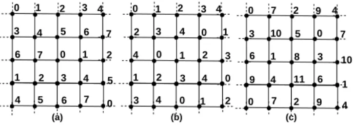
an optimal L(0, 1)-labeling for squared grids, that is reg-ular grids of degree 4 (see Figure (b)). Battiti, Bertossi and Bonuccelli (1) found an optimal L(1, 1)-labeling for hexagonal, squared and triangular grids (that is, respec-tively, regular grids of degree 3, 4 and 6, see Figures (a), (b) and (c)). The L(2, 1)-labeling problem of regular grids of degree ∆, denoted G∆, has been studied independently by different authors (3; 7) proving that λ2,1(G∆) = ∆ + 2 by means of optimal coloring algorithms. More recently, Fertin and Raspaud (10) determined several bounds on λh,kfor d-dimensional squared grids.
In (5) some values of λh,k for regular grids of degree 3, 4, and 6 are exactly computed, while in some intervals different upper and lower bounds are given ; moreover, the case h < k is not considered at all. Our goal in this paper is to improve some of those bounds, as well as to consider the case h < k. Moreover, we extend this study to a new class of graphs, namely grids of degree 8. Grids of degree 8 can be defined as the strong product of two infinite paths (15) (see also Figure for a graphical representation of the four types of grids we study in this paper). Grids of degree 8 can also be seen as a natural extension of grids of degree 6, who themselves are an extension of grids of degree 4 (see Figures (a), (b) and (c)).
Figure 1 Grids studied in this paper: (a) G3, (b) G4, (c) G6
and (d) G8
(a) (b)
(c) (d)
Before going further, we observe that when h < k (a case that we will consider in this paper), there are actually two ways to define the L(h, k)-labeling problem:
• The first one is the distance-based model, which asks that two neighbors in the graph differ by at least h, while two nodes at distance 2 differ by at least k. This means that when two nodes are at the same time con-nected by a 1-path and a 2-path (hence when there is a cycle of length 3 in the graph), we consider the distance to be 1, and thus impose only the condition on h.
• The second one is the max-based model, which asks that two nodes connected at the same time by a 1-path and a 2-1-path differ by at least max{h, k} ; in that
sense, this model is more restrictive than the distance-based model. In particular, this model imposes that any cycle of length 3 to be always labeled with three labels at least max{h, k} apart from each other. Note that when h ≥ k, the two definitions coincide, since max{h, k} = h. The same occurs when the considered graph has no triangles, which is the case for G3 and G4. In this paper, in the study of G6 and G8, when h < k, we chose to consider the max-based problem.
As mentioned above, we study in this paper the L(h, k)-labeling problem on regular grids of degree 3, 4, and 6 for those values of h and k whose λh,k is either not known or not tight, and we also study the L(h, k) labeling problem in a new class of graphs, namely grids of degree 8. For all considered grids, in some cases we provide exact results, or we give close upper and lower bounds (see Figure 6.2 at the end of the paper for a summary of results).
The paper is organized as follows: in Section , we give a few technical lemmas that will help to obtain general lower and upper bounds for the considered types of graphs, while in Sections , 3.2, 4.2 and 4.2, we improve bounds on the L(h, k) number of grids for degree 3, 4, 6 and 8, respec-tively.
Note finally that if no confusion arises, we will speak in-terchangeably, in the rest of this paper, of a node and its label.
2 PRELIMINARIES
In this section, we show four different lemmas, which will prove to be useful in the rest of the paper. Lemmas 1 and 1 are concerned with lower bounds for the L(h, k) num-ber, while Lemmas 2 and 3 deal with upper bounds. Theorem 1. λh,k(G∆) ≥ h + (∆ − 1)k when h ≤ k, for ∆ = 3, 4.
Proof. Consider an optimal L(h, k)-labeling of G∆, h ≤ k, ∆ = 3, 4, and let x be a node labeled 0. The smallest label among those of its neighbors must be at least h. Further-more, the ∆ neighbors of x are all connected by a 2-length path and hence their labels must differ by at least k from each other. It follows that the greatest label must be at least h + (∆ − 1)k.
Lemma 1. λh,k(G∆) ≥ ∆k when h ≤ k, for ∆ = 6, 8. Proof. Observe that G6 and G8 are characterized by the property that each pair of adjacent nodes is also connected by a 2-length path. This implies that, given an optimal L(h, k)-labeling of G∆, h ≤ k, ∆ = 6, 8, starting from a node x labeled 0, the smallest label, among those of their neighbors must be at least k. With reasonings analogous to those of the previous proof, the claim follows.
Lemma 2. For any graph G and any h ≤ k, λh,k(G) ≤ k· λ1,1(G).
Proof. Consider an optimal L(1, 1)-labeling, say L, of G. Consider the labeling L0 obtained from L by substituting every label i with label ik (i = 0, 1, . . . , λ1,1(G)). We claim that L0 is an L(h, k)-labeling of G with span k · λ1,1(G), provided h ≤ k. Indeed, any two neighbors, which differ by at least 1 in L, differ by at least k ≥ h in L0 ; moreover, any two nodes connected by a 2-length path, which differ by at least 1 in L differ by at least k in L0.
Lemma 3. For any graph G and any h ≥ k
2, λh,k(G) ≤ h· λ1,2(G).
Proof. Analogously to the proof of Lemma 2, consider an L(1, 2) labeling, say L, of G. Consider the labeling L0 obtained from L by substituting every label i with label ih (i = 0, 1, . . . , λ1,2(G)). Since h ≥ k
2, L0 is an L(h, k)-labeling of G with span h · λ1,2(G). Indeed, any two neigh-bors, which differ by at least 1 in L, differ by at least h in L0; moreover, any two nodes connected by a 2-length path, which differ by at least 2 in L differ by at least 2h ≥ k in L0.
3 REGULAR GRIDS OF DEGREE 3
3.1
Upper Bounds for G
3Proposition 1. λh,k(G3) ≤ h + 2k when h ≤ k 2.
Proof. Consider an optimal L(1, 2)-labeling of G3over the set of labels {0, 1, . . . , 5}, whose general pattern is depicted in Figure 3.1(a). The idea is to substitute h to 1, k to 2, h+k to 3, 2k to 4, and h+2k to 5. In that case, the labeling that is produced is a feasible L(h, k)-labeling. Indeed, each pair of consecutive labels differs by either h or k − h, but since we supposed h ≤ k
2, we have k − h ≥ h and thus any two consecutive labels differ by at least h. Similarly, any other pair of distinct labels differs by at least k. Moreover, the largest label used is h + 2k, hence the result.
Figure 2 General patterns for L(h, k)-labelings of G3:
(a) L(1, 2)-labeling ; (b) L(1, 1)-labeling
(a) 0 1 2 5 0 4 3 3 5 0 1 4 1 2 2 4 3 5 0 4 2 1 5 3 (b) 1 2 0 0 3 0 3 1 0 2 1 0 3 2 3 1 2 0 1 3 2 1 3 2
Proposition 2. λh,k(G3) ≤ min {5h, 3k} when k2 ≤ h ≤ k.
Proof. By Lemma 3, since k
2 ≤ h and since there exists an L(1, 2)-labeling of G3that is of span 5 (see for instance the general pattern shown in Figure 3.1(a)), we know there exists an L(h, k)-labeling of G3 of span 5h.
Analogously, since h ≤ k, we obtain an L(h, k)-labeling of span 3k by Lemma 2 ; indeed, there exists an L(1, 1)-labeling of G3 that is of span 3 (whose general pattern is shown in Figure 3.1(b), see also (1)).
3.2
Lower Bounds for G
3Proposition 3. λh,k(G3) ≥ h + 2k when h ≤ k. Proof. This bound directly comes from Lemma 1. Figure 3 Neighborhood of a node labeled 0 in G3
Proposition 4. λh,k(G3) ≥ 3k when 2k
3 ≤ h ≤ k.
Proof. Consider an optimal L(h, k)-labeling of G3. Sup-pose, by contradiction, that λh,k(G3) < 3k. Let us consider a node labeled 0, and let x, y, and z be its 3 neighbors. Without loss of generality, suppose x < y < z. In view of the L(h, k)-constraints, we must have x ≥ h, y≥ x + k ≥ h + k, and z ≥ y + k ≥ h + 2k. Furthermore, from the hypothesis λh,k(G3) < 3k, we have that z < 3k, hence y ≤ z − k < 2k, and x ≤ y − k < k. Let x1and x2, y1 and y2, z1 and z2 be the not 0 neighbors of x, y, and z, respectively (see Figure 3.2).
Let us first prove that if ym = min{y1, y2} and yM = max{y1, y2}, then ym < y < yM. Indeed, if y < ym, then ym ≥ y + h ≥ 2h + k, and consequently yM ≥ 2h + 2k. However, 2h + 2k ≥ 3k (because we supposed h ≥ 2k3 ≥
k
2), a contradiction to the fact that λ <3k. On the other hand, if yM < y, then y ≥ yM + h. And since yM ≥ ym+ k ≥ 2k, we end up with y ≥ h + 2k. However, by hypothesis we know that y < 2k, a contradic-tion since h ≥ 0. Thus we conclude that in all the cases, we have ym< y < yM.
Now, in order to prove the statement, we will show that under the hypothesis λh,k(G3) < 3k, both cases x1 < x2 and x1> x2lead to a contradiction.
Case 1: x1 < x2. In this case x1 ≥ k, as x1 is connected by a 2-length path to node 0 (via x) and x2 ≥ x1+ k ≥ 2k. If x1 < x, then x ≥ x1+ h ≥ k + h, a contradiction since x < k. Hence, x < x1 < x2. It follows that x1 ≥ x + h ≥ 2h and x2≥ x1+ k ≥ 2h + k. Let us now consider y1and y2.
Case 1.1: y1 < y2. Hence we know that y1 < y < y2.
In such a case y1≥ k and y1≤ y − h < 2k − h. Note that y1 < x2 as y1<2k − h and x2 ≥ 2k. Let us consider the common neighbor of x2 and y1, α, and let us study the relative position of its label with respect to x2 and y1.
• α < y1< x2. Then α ≤ y − k < k: if x < α we have α≥ x+k ≥ h+k, a contradiction ; on the other hand, if α < x then α ≤ x − k < 0, a contradiction too. • y1 < x2 < α. Then x2 ≤ α − h < 3k − h ; from
previous hypotheses we also have x2 ≥ 2h + k, and this leads to a contradiction as 3k − h ≤ 2h + k when h≥2k3.
• y1< α < x2. We have again two cases. If y1< α < y then α ≤ y − k < k and y1 ≤ α − h < k − h that is a contradiction as y1 ≥ k. If y1 < y < α then α ≤ x2 − h < 3k − h, y ≤ α − k < 2k − h, and y1≤ y − h < 2k − 2h that is a contradiction as y1≥ k and k ≥ 2k − 2h when 2k
3 ≤ h ≤ k.
Case 1.2: y1 > y2. Thus we have y1 > y > y2. This implies that y1 ≥ y + h ≥ 2h + k. Hence, y1 lies in the interval [2h + k; 3k[. However, we also know that x2 lies in the interval [2h + k; 3k[. Since this interval is of width w <2k−2h, we conclude that w < k (because we supposed h≥ 2k3 and hence h ≥
k
2). This leads to a contradiction because y1and x2must be at least k away from each other. Case 2: x1 > x2. With considerations analogous to those done for case x1 < x2, we can derive x < x2 < x1 and 2h + k ≤ x1<3k and 2h ≤ x2<2k. Now, let us look at y1 and y2.
Case 2.1: y1 < y2. We thus have y1 < y < y2. However, this leads to a contradiction. Indeed, y1 > k as it is connected by a 2-length path to node 0, then x2≥ y1+ k > 2k.
Case 2.2: y1 > y2. We then have y2 < y < y1. This implies that y1 ≥ y + h ≥ 2h + k and hence y1 > x2 as x2<2k. Now consider α, the common neighbor of x2 and y1.
• x2 < y1 < α. Then α ≥ y1+ h ≥ 3h + k ≥ 3k, a contradiction since we supposed λ < 3k.
• α < x2 < y1. Then α ≤ x2− h < 2k − h. If α > y then α ≥ y + k ≥ h + 2k, a contradiction ; if α < y then α ≤ y − k ≤ k. However, we know that x < k ; moreover, because α < k and α must lie at least k away from x, this leads to a contradiction.
• x2< α < y1. Then α ≤ y1−h < 3k −h. If α > y then α≥ y + k ≥ h + 2k that is greater than 3k − h under the hypothesis h ≥ 2k
3, a contradiction ; if α < y then α≤ y − k ≤ k that again contradicts the fact that α must lie at least k away from x.
Altogether, we see that every possible case leads to a contradiction. This proves that the initial assumption, λ < 3k, is false, and consequently the proposition is proved.
Proposition 5. λh,k(G3) ≥ 3h when k ≤ h ≤3k 2.
Proof. The proof is analogous to the previous one, i.e., by contradiction we assume that there exists a L(h, k)-labeling with span λ < 3h, we start from node labeled 0, we look at its neighbors and prove that neither x1 < x2 nor x1 > x2 can occur. Wlog, let us assume x < y < z. Hence, x ≥ h, y ≥ h + k and z ≥ h + 2k. On the other hand, z < 3h, y < 3h − k and x < 3h − 2k. Let x1 and x2, y1 and y2, z1 and z2 be the not 0 neighbors of x, y, and z, respectively (see Figure 3.2).
We first prove that if ym = min{y1, y2} and yM = max{y1, y2}, then ym < y < yM. Indeed, if y < ym, then ym ≥ y + h ≥ 2h + k, and consequently yM ≥ 2h + 2k. However, 2h + 2k ≥ 3h (because we supposed h ≤3k2 ), a contradiction to the fact that λ < 3h. On the other hand, if yM < y, then y ≥ yM+ h. And since yM ≥ ym+ k ≥ 2k, we end up with y ≥ h + 2k. However, by hypothesis we know that y < 3h − k, a contradiction since 3h − k ≤ h + 2k, because we supposed h ≤ 3k
2. Thus we conclude that in all the cases, we have ym < y < yM. Now, as in the previous proof, let us consider x1 and x2 (see Figure 3.2), and show that, under the hypothesis λ <3h, none of the cases x1< x2 and x1> x2 can occur. Case 1: x1 < x2. This implies x1 ≥ k, as x1 is connected by a 2-length path to node 0 (via x). If x1< x, then x ≥ x1 + h ≥ h + k, that is a contradiction as x <3h − 2k ≤ h + k under the hypothesis h ≤ 3k
2 . Hence, x < x1 < x2. It follows that x1 ≥ x + h ≥ 2h and x2≥ x1+ k ≥ 2h + k. Let us consider now y1and y2.
Case 1.1: y1 < y2. Then we know that y1 < y < y2. Note that y1< x2as x2≥ 2h+k and y1≤ y−h ≤ y2−2h < 3h − 2h = h. Now, let us consider α, the common neighbor of y1 and x2.
• y1 < x2 < α. The contradiction comes from the in-equality α ≥ x2+ h ≥ 3h + k.
• α < y1< x2. Then y1≥ α + h ≥ h, y ≥ y1+ h ≥ 2h and y2≥ y + h ≥ 3h, a contradiction.
• y1 < α < x2. Since we have y1 ≥ k, this implies α≥ y1+ h ≥ h + k and α ≤ x2− h < 2h. It is easy to see that the same bounds hold also for y. Hence y and α both lie in the interval [h + k; 2h[, of width w < h− k, that is w ≤ k. The contradiction comes from the fact that α and y being connected by a 2-length path, they must lie at least k away from each other.
Case 1.2: y1 > y2. Thus, we know that y1 > y > y2. We know that x2and y1must be at least k away from each other. Moreover, 2h + k ≤ x2<3h and 2h + k ≤ y1<3h. Hence, both x2and y1lie in an interval of width w < h−k. Since we supposed h ≤ 3k
2, we conclude w < k, a contra-diction.
Case 2: x1 > x2. We can easily see that in that
case we must have x1 > x2 > x. Indeed, x2 ≥ k, since it is connected by a 2-length path to node 0. Hence, if x > x2, then x ≥ h + k. However, we know that x < 3h − 2k, a contradiction since h ≤ 3k
2. Hence we conclude that x1> x2> x, which implies x2≥ x + h ≥ 2h and x1≥ x2+ k ≥ 2h + k. Now let us consider y1 and y2. Case 2.1: y1 < y2. Let us then consider α, the common neighbor of y1 and x2, and let us look at its relative position compared to x and y. There are three possible cases.
• α > y > x. We recall that we are in the case x1 > x2 > x, that is x2 ≥ x + h ≥ 2h. If α > x2 then α ≥ x2+h ≥ 3h, a contradiction to the hypothesis λ < 3h. Now, if α < x2, α ≤ x2−h. Since x2≤ x1−k < 3h−k, we conclude α ≤ 2h − k. But y ≥ h + k and α ≥ y + k, that is α ≥ h + 2k. This is a contradiction since 2h − k ≤ h + 2k, by the hypothesis that h ≤ 3k2. • y > α > x. We then conclude that α ≤ y−k < 3h−2k.
On the other hand, we have α ≥ x + k ≥ h + k. This is a contradiction since h + k ≥ 3h − 2k due to the fact that we supposed h ≤3k
2.
• y > x > α. In that case, if α < y1, then y1≥ α + h ≥ h, which implies y ≥ 2h and y2≥ 3h, a contradiction to the hypothesis λ < 3h. Now, if α > y1, then α ≥ h, which in turns means that x ≥ h + k and y ≥ h + 2k. However, we know that y < 3h − k, a contradiction since 3h − k ≤ h + 2k due to the fact that we supposed h≤3k
2.
Case 2.2: y1 > y2. Here, we consider the three nodes z, z1 and z2. We first show that if zm = min{z1, z2} and zM = max{z1, z2}, then zm< zM < z. Indeed, if zM > z then zM ≥ z + h, and since we know z ≥ h + 2k, we conclude zM ≥ 2h + 2k, a contradiction to the fact that λ <3h since 2h + 2k ≥ 3h. Now let us look at the relative positions of z1and z2. There are two cases to consider.
• z1> z2. In that case, we have z > z1> z2. Now let us look at β, common neighbor of z1 and y2, and let us consider the relative positions of β and y.
– β < y. First, we note that β < z1. Indeed, z2≥ k (it is connected by a 2-length path to node 0), thus z1≥ 2k. However, β < y by hypothesis, hence β ≤ y − k, that is β < 2h − k. Moreover, 2h − k ≤ 2k since we are in the case h ≤ 3k
2, and thus we conclude that β < z1. This implies β≤ z1−h, that is β ≤ z −2h ; and since z ≤ λ < 3h, we get β < h. On the other hand, y2 < y, thus y2 ≤ y − h. But since y < 2h, we then have y2 < h. Hence, both β and y2 lie in the interval [0; h[. However, they are neighbors and thus should have labels that are at least h away, a contradiction.
– β > y. Then we have β ≥ y + k, that is β ≥ h+ 2k. However, we know that z ≥ h + 2k as
well. Thus, β and z lie in the interval [h + 2k; λ[, where λ < 3h by hypothesis. Thus the width of this interval w satisfies w < 2h − 2k, and thus w < kbecause we supposed h ≤ 3k
2. However, β and z are neighbors, and thus should have labels at least differing by h, a contradiction with the fact that w < h.
• z2> z1. In that case, we know that z > z2 > z1. In particular, this means that z2<2h, and z1<2h − k. However, z1 ≥ k since it is connected by a 2-length path to node 0. We also have y ≤ z −h < 2h, and thus y2 ≤ y − h < h ; and since h ≥ k, we conclude that y2≤ 2h − k. Moreover, y2≥ k since it is connected by a 2-length path to node 0. Hence, both z1 and y2 lie in the interval [0; 2h − k[, of width w < 2h − 2k, that is w < k since we supposed h ≤ 3k2. However, z1 and y2 are connected by a 2-length path, and thus should have labels at least differing from k, a contradiction. Altogether, we see that every possible case leads to a contradiction. This proves that the initial assumption, λ < 3h, is false, and consequently the proposition is proved. Proposition 6. λh,k(G3) ≥ h + 3k when 3k2 ≤ h ≤ 2k. Proof. Consider an optimal L(h, k)-labeling of G3 with span λ. By contradiction, suppose λ < h + 3k. Let us consider a node labeled 0, and let x, y, and z be its 3 neighbors. Without loss of generality, suppose x < y < z. In view of the L(h, k)-constraints, we must have x ≥ h, y≥ x + k ≥ h + k, and z ≥ y + k ≥ h + 2k. Furthermore, for the hypothesis λ < h + 3k, z < h + 3k, hence y≤ z − k < h + 2k, and x ≤ y − k < h + k. Let x1and x2, y1 and y2, z1 and z2 be the not 0 neighbors of x, y, and z, respectively (see Figure 3.2).
Let us first prove the following, which will be useful in the rest of the proof: if ym = min{y1, y2} and yM = max{y1, y2}, then ym < y < yM. Indeed, if y < ym < yM, we have ym ≥ y + h ≥ 2h + k, and yM ≥ ym+ k ≥ 2h + 2k. However, this contradicts the fact that λ < h + 3k, because 2h + 2k ≥ h + 3k (since we supposed h ≥ 3k
2). Now suppose ym < yM < y. Then ym≥ k, because it is connected by a 2-length path to node 0. Thus yM ≥ ym+ k ≥ 2k, and y ≥ yM + h ≥ h + 2k, which contradicts the fact that y < h + 2k. Altogether, we conclude that the only possible case is ym< y < yM (1). In the following we show that, under the hypothesis λ < h+ 3k, both cases x1 < x2 and x1 > x2 lead to a contradiction, which will prove the statement.
Case 1: x1 < x2. This implies x1 ≥ k, as x1 is connected by a 2-length path to node 0 (via x) and x2 ≥ x1+ k ≥ 2k. If x1 < x, then x ≥ x1+ h ≥ k + h, that is a contradiction as x < h + k. Hence, we have x < x1 < x2. It follows that x1 ≥ x + h ≥ 2h and x2 ≥ x1+ k ≥ 2h + k. Moreover, x1 ≤ x2− k < h + 2k and x ≤ x1− h < 2k. Let us now consider y1and y2.
Case 1.1: y1< y2. By (1) above, we have y1< y < y2. Let us now consider α (common neighbor of y1 and x2), and let us study its relative position compared to x and y (we recall that x < y by hypothesis).
• α > y > x. Hence we have α ≥ y + k ≥ h + 2k. But x2 ≥ 2h + k ≥ h + 2k as well. Hence, both α and x2 lie in the interval [h + 2k; h + 3k[, of width w < k ≤ h. However, x2 and α are neighbors, thus they must be at least h away, a contradiction.
• y > α > x. In that case, α ≤ y − k < 2k. But we also have α ≥ x + k ≥ h + k, a contradiction.
• y > x > α. Since x < 2k, we conclude that α ≤ x− k < k. However, we know y1 ≥ k (because it is connected by a 2-length path to node 0). Thus α < y1, hence y1≥ α + h ≥ h. But we know y1< y < y2, thus y1 ≤ y − h, and y ≤ y2− h < 3k, thus y1 <3k − h. But we cannot have y1 ≥ h and y1 <3k − h, since h≥3k
2.
Case 1.2: y2< y1. By (1) above, we have y2< y < y1. Hence y1≥ y +h ≥ 2h+k. We also know that x2≥ 2h+k, since x < x1< x2. Thus y1and x2share the same interval [2h + k; h + 3k[, of width w < 2k − h ≤ k. But y1 and x2 are connected by a 2-length path, and thus must be at least k away, which is impossible.
Hence, at this point we conclude that necessarily x1> x2. Thus let us consider this case.
Case 2: x2 < x1. In that case, it is easily seen that actually x1 > x2 > x, since x > x2 would imply x ≥ x2 + h ; and since x2 ≥ k (it is connected by a 2-length path to node 0), we would have x ≥ h + k, a contradiction to the fact that x < h + k. Now let us look again at the relative positions of y1 and y2.
Case 2.1: y1< y2. By (1) above, we have y1< y < y2. This implies that y ≤ y2− h < 3k. And since we know by hypothesis that x < y, we conclude that x ≤ y − k < 2k.
• α > y > x. Then α ≥ y + k ≥ h + 2k. However, we know x2< x1, that is x2≤ x1− k < h + 2k, hence we conclude α > x2. Thus α ≥ x2+ h, and since x2> x we have x2 ≥ x + h ≥ 2h, we conclude α ≥ 3h, a contradiction to the fact that λ < h + 3k, since we supposed h ≥ 3k
2.
• y > α > x. Then α ≥ x + k ≥ h + k, and α ≤ y− k < 2k. This is a contradiction since h + k ≥ 2k by hypothesis.
• y > x > α. Then α ≤ x − k < k. However, y1 ≥ k (it is connected by a 2-length path to node 0). Thus y1 > α, which means y1 ≥ α + h ≥ h. But we know that y1 < y, that is y1 ≤ y − h < 3k − h. This is a contradiction since h ≥ 3k − h by hypothesis.
Case 2.2: y1> y2. By (1) above, we have y2< y < y1. Let us now look at the relative positions of z, z1and z2. We
first note that if zm= min{z1, z2} and zM = max{z1, z2}, then zm< zM < z. Indeed, if zM > z then zM ≥ z + h, and since we know z ≥ h + 2k, we conclude zM ≥ h + 3k, a contradiction.
• z1> z2. Hence z > z1> z2, by the argument above. Let us derive here some inequalities that will be useful in the following. Since z < h + 3k and z1≤ z − h, we conclude z1<3k. Moreover, we know that z2≥ k and z1> z2, thus we conclude z1 ≥ z2+ k ≥ 2k. Finally, we recall that h + 2k ≤ z < h + 3k. Now let us look at the relative positions of β and y.
– β < y. Then β ≤ y − k < 2k. Since z1 ≥ 2k, we conclude β < z1. Thus β ≤ z1− h ≤ 3k − h. We also know that y2≤ 3k − h because y2< y≤ y− h, and because y < 3k. Hence, both β and y2 are contained in the interval [0; 3k − h[, of width w <3k − h. But 3k − h ≤ h by hypothesis, and since β and y2 must be at least h away, this is impossible.
– β > y. Then β ≥ y + k ≥ h + 2k. This implies that both β and z lie in the interval [h + 2k; h + 3k[, of width w < k. However, β and z must be at least k away from each other, a contradiction. • z2 > z1. Hence z > z2 > z1. In particular, we have k≤ z1<2k. But we also know that k ≤ y2<3k−h ≤ 2k. Thus y2 and z1 both lie in the interval [k; 2k[, of width w < k. But they must be at least k away, a contradiction.
Altogether, we have shown that every possible case leads to a contradiction. This proves that the initial assumption, λ < h+ 3k, is false. This proves the proposition.
4 REGULAR GRIDS OF DEGREE 4
4.1
Upper Bounds for G
4Proposition 7. λh,k(G4) ≤ h + 3k when h ≤ k 2.
Proof. Consider the L(1, 2)-labeling whose general pattern is depicted in Figure 4.1(a). This labeling has span 7. If we now substitute labels 0, h, k, h + k, 2k, h + 2k, 3k, h + 3k to labels 0, 1, . . . , 7, the new labeling we obtain is an L(h, k)-labeling of G4. Indeed, it is easy to see that when h ≤
k
2, each pair of consecutive labels differs by at least h, while each other pair of distinct labels differs by at least k. Moreover, the largest label used is h + 3k, hence the result.
Proposition 8. λh,k(G4) ≤ min {7h, 4k} when k2 ≤ h ≤ k.
Figure 4 General patterns for L(h, k)-labelings of G4:
(a) L(1, 2) ; (b) L(1, 1) ; (c) L(3, 2) 3 4 5 6 7 6 7 0 1 2 1 4 2 3 4 5 5 6 7 0 2 4 1 3 3 0 2 4 4 1 3 0 1 2 2 4 0 3 0 1 3 6 9 0 10 1 4 7 5 8 11 2 0 7 10 1 4 3 6 9 (a) (b) (c) 0 1 2 3 4 0 1 2 3 4 0 7 2 9 4
Proof. By Lemma 3, since k
2 ≤ h and since there exists an L(1, 2)-labeling of G4 that is of span 7 (as shown in Figure 4.1(a)), we know there exists an L(h, k)-labeling of G4of span 7h.
Analogously, since h ≤ k, we obtain an L(h, k)-labeling of span 4k by Lemma 2 ; indeed, there exists an L(1, 1)-labeling of G4that is of span 4 (whose pattern is shown in Figure 4.1(b), see also (1)).
Proposition 9. λh,k(G4) ≤ 3h + k when 3k 2 ≤ h ≤
5k 3. Proof. Consider the L(3, 2)-labeling of G4 whose general pattern is depicted in Figure 4.1(c). This labeling has span 11. If we now substitute labels 0, h − k, k, h, 2h − k, h + k,2h, 3h − k, 2h + k, 3h, 4h − k, 3h + k to labels 0, 1, . . . , 11, the new labeling we obtain is an L(h, k)-labeling of G4. By construction, any pair of labels that are at least 3 away in the list differs by at least h, while any pair of labels that is at least 2 away in the list differs by at least k, because we supposed 3k2 ≤ h. Moreover, the largest label used is 3h + k, hence the result.
Proposition 10. λh,k(G4) ≤ 11k 2 when 11k 8 ≤ h ≤ 3k 2. Proof. It is known (see (5)) that λh,k(G4) ≤ 4h when h ≥ k. Since λh,k is a non decreasing function, Proposition 9 implies that λh,k(G4) ≤11k 2 when 11k 8 ≤ h ≤ 3k 2.
4.2
Lower Bounds for G
4Proposition 11. λh,k(G4) ≥ h + 3k when h ≤ k. Proof. This bound directly comes from Lemma 1.
5 REGULAR GRIDS OF DEGREE 6
Proposition 12. λh,k(G6) = 6k when h ≤ k.
Proof. The upper bound is proved observing that since h ≤ k, we obtain an L(h, k)-labeling of span 6k by Lemma 2 ; indeed, there exists an L(1, 1)-labeling of G6 of span 6, whose general pattern is shown in Figure 4.2 (see also (1)). The lower bound directly comes from Lemma 1.
Figure 5 General pattern of an L(1, 1)-labeling of G6of span 6 0 1 2 3 4 3 4 5 6 2 6 0 1 5 4 6 1 0 1 2 3 2 3 4 5
6.1
Upper Bounds for G
8Proposition 13. λh,k(G8) ≤ 8k when h ≤ k.
Proof. Since h ≤ k, we obtain an L(h, k)-labeling of span 8k by Lemma 2 ; indeed, there exists an L(1, 1)-labeling of G8 of span 8 (whose general pattern shown in Fig-ure 6.1(a)).
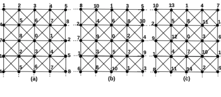
Figure 6 General patterns for L(h, k)-labelings of G8:
(a) L(1, 1) ; (b) L(2, 1) ; (c) L(3, 1) (a) 1 4 7 1 4 2 4 5 5 6 7 8 2 5 8 8 2 5 0 3 6 1 4 7 3 10 13 1 4 7 2 5 8 11 14 9 12 0 3 6 1 4 7 10 13 8 11 14 2 9 8 10 1 3 5 2 4 6 8 10 7 9 0 2 4 3 5 7 9 1 6 1 8 10 3 (b) (c)
Proposition 14. λh,k(G8) ≤ min {8h, 10k} when k ≤ h≤ 2k.
Proof. Once again we exploit the L(1, 1)-labeling of G8 whose general pattern is depicted in Figure 6.1(a). If we substitute 0, h, 2h, . . . 8h to labels 0, 1, . . . , 8, the new la-beling we obtain is an L(h, k)-lala-beling of G8. Indeed, it is easy to see that each pair of consecutive labels differs by at least h, and thus by at least k since k ≤ h. Moreover, the largest label used is 8h, hence the result.
The upper bound of 10k comes from the L(2, 1)-labeling of G8 whose general pattern is shown in Figure 6.1(b). If we substitute 0, k, 2k, . . . 10k to labels 0, 1, . . . , 10, the new labeling we obtain is an L(h, k)-labeling of G8. Indeed, it is easy to see that when k ≤ h ≤ 2k, each pair of non consecutive labels differs by at least 2k ≥ h, while any pair of distinct labels differs by at least k. Moreover, the largest label used is 10k, hence the result.
Proposition 15. λh,k(G8) ≤ min {5h, 14k} when 2k ≤ h≤ 3k.
Proof. Consider the L(2, 1)-labeling whose general pat-tern is described in Figure 6.1(b). This labeling has span 10. If we now substitute 0, k, h, h + k, 2h, 2h + k, 3h, 3h + k,4h, 4h + k, 5h to labels 0, 1, . . . , 10, the new labeling we
obtain is an L(h, k)-labeling of G8. Indeed, it is easy to see that each pair of non consecutive labels differs by at least h. On the other hand, since 2k ≤ h, any pair of distinct labels differs by at least k. Moreover, the largest label used is 5h.
Analogously, the other bound is given using an L(3, 1)-labeling, such as the one whose general pattern is shown in Figure 6.1(c). This labeling is of span 14. If we now substitute 0, k, 2k, . . . , 14k to labels 0, 1, . . . , 14, the new labeling we obtain is an L(h, k)-labeling of G8. Indeed, when h ≤ 3k, each pair of labels that are at least 3 away in the list differs by at least 3k ≥ h, while any pair of distinct labels differs by at least k. Moreover, the largest label used is 14k, hence the result.
Proposition 16. λh,k(G8) ≤ 4h + 2k when 3k ≤ h ≤ 6k. Proof. Starting from the L(3, 1)-labeling used in the pre-vious proof (cf. also Figure 6.1(c)) of span 14, we substi-tute labels 0, k, 2k, h, h + k, h + 2k, 2h, 2h + k, . . . , 4h, 4h + k,4h+2k to labels 0, 1, . . . , 14. This new labeling is also an L(h, k)-labeling of G8. Indeed, each pair of labels that are at least 3 away in the list differs by at least h by construc-tion, while any pair of distinct labels differs by at least k because h ≥ 3k. Moreover, the largest label used is 4h+2k, hence the result.
Proposition 17. λh,k(G8) ≤ 3h + 8k when h ≥ 6k. Proof. Consider the labeling whose general pattern is de-picted in Figure 6.1(a). This labeling is an L(1, 1)-labeling of span 11, with the additional property that the only con-secutive labels that can appear on neighboring nodes are of the form 3i + 2 and 3(i + 1). We now replace any label l of this labeling by a new label, thanks to the following rule (cf. Figure6.1(b)): any label of the form l = 3i + j (i = 0, 1, 2, 3, j = 0, 1, 2) is replaced by l0= (h + 2k)i + jk. In this new labeling, any pair of labels of the form 3i + 2 and 3(i + 1) is now separated by h. Moreover, the labeling we started from is an L(1, 1)-labeling, and any two differing labels in the new labeling are at least k away. Thus, this new labeling is an L(h, k)-labeling, of span 3h + 8k. Figure 7 (a) General pattern of an L(1, 1)-labeling of G8 ;
(b) general pattern of the L(h, k)-labeling we derive
0 3 6 9 0 7 10 1 4 7 2 6 1 4 7 10 1 9 0 3 6 2 5 8 11 0 h+2k 2h+4k 3h+6k 0 2h+5k 3h+6k 0 k k k h+3k h+3k 2k 2k 3h+7k 3h+7k 2h+6k h+4k 3h+8k h+2k 2h+4k 2h+5k 2h+5k 2h+4k
6.2
Lower Bounds for G
8Proof. This bound directly comes from Lemma 1. Proposition 19. λh,k(G8) ≥ 2h + 6k when k ≤ h ≤ 3k. Proof. Consider any optimal L(h, k)-labeling of G8. Let λ be the greatest label. Let us consider a label x which is neither 0 nor λ (note that there must exist one since G8 contains K3 as an induced subgraph ; note also that necessarily, x lies in the interval [h; λ − h]). Now, consider its 8 neighbors, say v1. . . v8. Then no other label than x can be used in the interval ]x−h; x+h[ for the vis. However, all the vis are pairwise connected by 2-length paths, so they must be at least k away from each other. If there are α (resp. β) labels for the vis in the interval [0; x − h] (resp. [x + h; λ]), then we must have (x − h) − (α − 1)k ≥ 0 and λ≥ (x+h)+(β −1)k, with α+β = 8. Since λh,k(G8) = λ, we conclude that λh,k(G8) ≥ 2h + (α + β − 2)k, hence the result.
Proposition 20. λh,k(G8) ≥ 3h + 3k when h ≥ 3k. Proof. First, observe that we have λh,k(G8) ≥ 3h + k. In-deed, consider an optimal L(h, k)-labeling of G8, a node labeled 0, and the set of its neighbors (see Figure 6.2). Wlog, suppose min{a, b, c} ≤ min{e, f, g}. Since a, b and c are neighbors of 0, then we have min{a, b, c} ≥ h. And since any node among e, f and g are connected by a 2-length path to any node among a, b and c, we conclude that min{e, f, g} ≥ h + k. Finally, since e, f and g induce a K3, we have max{e, f, g} ≥ 3h + k.
Figure 8 Neighborhood of a node labeled 0 in G8.
0 c g a b h e d f
However, we can derive a better lower bound of 3h + 3k, taking into account nodes d and h in ad-dition to the previous study. This bound then de-rives from a very tedious case by case analysis that is not developed here. Instead, we have run an ex-haustive search by computer on the grid restricted to those nine nodes. The source and binary codes cor-responding to this search are available at the following URL: http://www.sciences.univ-nantes.fr/info/perso/perma-nents/fertin/Lhk/Lhk.c).
7 CONCLUDING REMARKS
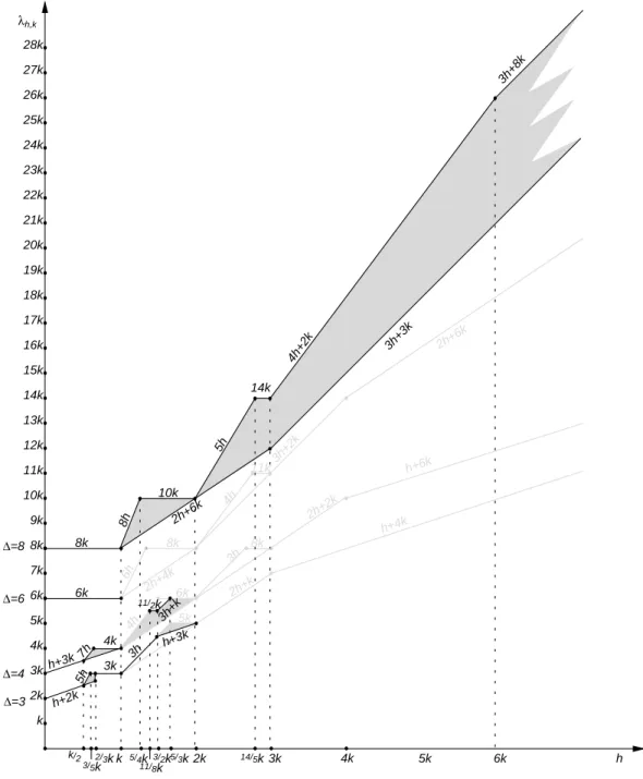
In this paper, we have studied the L(h, k)-labeling problem on regular grids of degree 3, 4, 6 and 8, and we have improved, in many different cases, the bounds on the L(h, k) number in each of these classes of graphs. A graph-ical representation of our results is depicted in Figure 6.2:
bold lines in this figure are results from this paper, grey lines are previously known results, and grey zones repre-sent the gaps that still exist between the known lower and upper bounds.
Though we managed to obtain tight bounds in several cases, there are still some other cases for which the gap is not closed, and it actually looks difficult to improve the bounds without using case by case analysis arguments, as we have sometimes done in this paper. However, a natural question consists in closing the gaps that still remain in all the four classes of graphs considered here.
Moreover, as observed in the introduction, when h < k we have considered in this paper the max-based model, that imposes a condition on labels of nodes connected by a 2-length path instead of using the concept of distance 2 (we recall that when h ≥ k, the two definitions coincide). Hence, it is also natural to ask for a similar study in the case h < k, but using this time the distance-based defi-nition. We note that this makes sense only for G6 and G8, since there are no triangles in G3 and G4, and thus in that case the two definitions coincide. Moreover, since the max-based model is by definition more restrictive than the distance-based model, the upper bounds we obtain in the max-based model also apply in the distance-based model, while this is not a priori the case for lower bounds.
REFERENCES
[1] R. Battiti, A.A. Bertossi and M.A. Bonuccelli. Assign-ing Codes in Wireless Networks: Bounds and ScalAssign-ing Properties. Wireless Networks, 5:195–209, 1999. [2] A.A. Bertossi and M.A. Bonuccelli. Code Assignment
for Hidden Terminal Interference Avoidance in Mul-tihop Packet Radio Networks. IEEE/ACM Trans. on Networking, 3:441–449, 1995.
[3] A.A. Bertossi, C.M. Pinotti and R.B. Tan. Channel assignment with separation for interference avoidance in wireless networks. IEEE Transactions on Parallel and Distributed Systems 14:222–235, 2003.
[4] H.L. Bodlaender, T. Kloks, R.B. Tan and J. van Leeuwen. λ-Coloring of Graphs. In Proc. of STACS 2000. LNCS 1770, 395–406, 2000.
[5] T. Calamoneri. Exact Solution of a Class of Frequency Assignment Problems in Cellular Networks and Other Regular Grids. Proc. 8th Italian Conference on The-oretical Computer Science (ICTCS’03), LNCS 2841, 163–173, 2003.
[6] T. Calamoneri. The L(h, k)-Labelling Problem: A Survey. Tech. Rep. 04/2004 Univ. of Rome “La Sapienza”, Dept. of Computer Science, 2004.
[7] T. Calamoneri and R. Petreschi. L(h, 1)-Labeling Subclasses of Planar Graphs. Journal on Parallel and Distributed Computing 64(3): 414-426, 2004.
Figure 9 Summary of the results achieved in this paper: bold lines are results from this paper, grey lines are previously known results, and grey zones represent the gaps that still exist between the known lower and upper bounds.
λh,k k 2k 3k 4k 5k 6k 7k 8k 9k 10k 11k 12k 13k 14k 15k k 3/2k 2k 3k 4k 2h+6 k 3h+2 k 8k 6h ∆=6 2h+2 k 6k 4h ∆=4 3h 3h ∆=3 2h+k 5k 5/3k 4h h+4k 11k 8k h+6k 2h+4 k h+2k k/2 2/3k 3/5k 3k 5h h+3k h+3k 7 h 11/2k 3h+k 6k ∆=8 8k 2h+6 k 10k 8h 5/4k 14k 5h 4h+ 2k 14/5k 11/8k 16k 17k 5k 6k h 18k 19k 20k 21k 22k 3h+8 k 3h+3 k 23k 24k 25k 26k 27k 28k 4k
[8] G.J. Chang, W.-T. Ke, D. Kuo, D.D.-F. Liu and R.K. Yeh. On L(d, 1)-labelings of graphs. Discrete Mathe-matics 220:57–66, 2002.
[9] G.J. Chang and D. Kuo. The L(2, 1)-labeling Problem on Graphs. SIAM J. Disc. Math., 9:309–316, 1996. [10] G. Fertin and A. Raspaud. L(p, q) Labeling of
d-Dimensional Grids. Discrete Applied Mathematics, to appear.
[11] J.R. Griggs and R.K. Yeh. Labeling graphs with a Condition at Distance 2. SIAM J. Disc. Math, 5:586– 595, 1992.
[12] W.K. Hale. Frequency assignment: theory and appli-cations. Proc. IEEE, 68:1497–1514, 1980.
[13] P.K. Jha, A. Narayanan, P. Sood, K. Sundaram and V. Sunder. On L(2, 1)-labeling of the Cartesian prod-uct of a cycle and a path. Ars Combin. 55:81–89, 2000. [14] P.K. Jha. Optimal L(2, 1)-labeling of Cartesian prod-ucts of cycles with an application to independent dom-ination. IEEE Trans. Circuits & Systems I: Funda-mental Theory and Appl. 47:1531–1534, 2000. [15] D. Korˇze and A. Vesel. L(2,1)-labeling of strong
prod-ucts of cycles. Information Processing Letters 94:183-190, 2005.
[16] T. Makansi. Transmitter-Oriented Code Assignment for Multihop Packet Radio. IEEE Trans. on Comm., 35(12):1379–1382, 1987.
[17] B.H. Metzger. Spectrum Management Technique. In Proc. 38th National ORSA Meeting, LNCS 1770, 395– 406, 1970.
[18] M. Molloy and M.R. Salavatipour. Frequency channel assignment on planar networks. In Proceedings of 10th Annual European Symposium on Algorithms (ESA), LNCS 2461, 736–747, 2002.
[19] D. Sakai. Labeling Chordal Graphs: Distance Two Condition. SIAM J. Disc. Math, 7:133–140, 1994. [20] M.A. Whittlesey, J.P. Georges and D.W. Mauro. On
the λ number of Qn and related graphs, SIAM J. Discr. Math. 8:499-506, 1995.