2011 — Calibration of a serial robot using a laser tracker

(1)

ÉCOLE DE TECHNOLOGIE SUPÉRIEURE UNIVERSITÉ DU QUÉBEC

MÉMOIRE PRÉSENTÉ À

L’ÉCOLE DE TECHNOLOGIE SUPÉRIEURE

COMME EXIGENCE PARTIELLE À L’OBTENTION DE LA MAÎTRISE EN GÉNIE DE LA PRODUCTION AUTOMATISÉ M.Ing. PAR Albert NUBIOLA

CALIBRATION OF A SERIAL ROBOT USING A LASER TRACKER

(2)

Cette licence signifie qu’il est interdit de reproduire, d’enregistrer ou de diffuser en tout ou en partie, le présent document. Le lecteur qui désire imprimer ou conserver sur un autre media une partie importante de ce document, doit obligatoirement en demander l’autorisation à l’auteur.

(3)

PRÉSENTATION DU JURY CE MÉMOIRE A ÉTÉ ÉVALUÉ

PAR UN JURY COMPOSÉ DE

M. Ilian Bonev, directeur de mémoire

Département de génie de la production automatisée à l’École de technologie supérieure

M. Vincent Duchaine, président du jury

Pascal Bigras, membre du jury

IL A FAIT L’OBJET D’UNE SOUTENANCE DEVANT JURY ET PUBLIC LE 15 JUILLET 2011

(4)

(5)

ACKNOWLEDGEMENTS

I would like to thank my supervisor Prof. Ilian Bonev for his constant support and motivation to keep me working on my studies. He gave me all the necessary means and equipment to complete my project.

I would like to thank Dr. Torgny Brogardh, from ABB headquarters, for his comments and suggestions on our results. I would also like to thank Dr. Mohamed Slamani for his help.

I thank my family for their support. My mother, Judith, and my father, Jordi, always took care of me and gave me the right advice at the right time. Thanks to my parents I ended up studying in the field of robotics.

Last but not least I thank Lauren, for her loving support and patience helping me to improve my English. Thanks to Lauren it was much easier for me to write this thesis.

(6)

VI

ÉTALONNAGE D’UN ROBOT SÉRIEL AVEC UN SYSTÈME DE LASER DE POURSUITE

Albert NUBIOLA RÉSUMÉ

La performance en positionnement d’un robot industriel ABB IRB 1600-6/1.45 a été étudiée avec un système de laser de poursuite (« laser tracker »). En faisant l’analyse axe par axe, on trouve que les axes 2, 3 et 6 ont un comportement non géométrique. Un modèle à 34 paramètres d’erreur a été utilisé pour modéliser le robot réel. Ce modèle d’erreur tient en compte les défauts géométriques de fabrication ainsi que quatre paramètres d’erreur concernant la rigidité (provenant des axes 2 et 3) et quatre autres paramètres d’erreur pour modéliser le comportement non linéaire du sixième axe avec une série de Fourier de deuxième ordre. L’algorithme d’optimisation non linéaire Nelder-Mead a été utilisé pour trouver les paramètres d’erreur qui correspondent aux mesures prises du robot.

Une fois les 34 paramètres identifiés, on ne peut pas appliquer une solution algébrique pour calculer la cinématique inverse du modèle à 34 paramètres d’erreur. On propose une solution numérique itérative à la cinématique inverse. Au maximum trois itérations sont nécessaires pour obtenir les angles des moteurs correspondants à une pose de l’outil.

Pour comparer la précision entre le modèle nominal et le modèle corrigé (à 34 paramètres d’erreur) on a fait des tests similaires à ceux proposés dans la norme ISO 9283. La validation de l’amélioration de la précision absolue est faite avec de nombreuses mesures. Pour le modèle à 34 paramètres, l’erreur de position moyenne/maximale est réduite de 0.979 mm / 2.326 mm à seulement 0.329 mm / 0.916 mm (vérification faite avec environ 1000 mesures arbitraires), avec une charge de l’outil de 6 kg (soit, le maximum), pour huit points sur l’outil et pour tout l’espace de travail du robot (ou presque, car il y avait quelques obstacles proches du robot à éviter).

On a fait des analyses avec l’erreur attendue, qui permettent de « prévalider » les modèles sans devoir prendre plus de mesures. On trouve que cette « prévalidation » est proche à la validation réelle.

Mots-clés : étalonnage robotique, laser tracker, erreur de position, erreur d’orientation, cinématique inverse, paramètres d’erreur, optimisation, IRB1600-6/1.45, ISO 9283.

(7)

VII

CALIBRATION OF A SERIAL ROBOT USING A LASER TRACKER Albert NUBIOLA

ABSTRACT

The positioning performance of an industrial robot ABB IRB 1600-6/1.45 has been studied with a laser tracker. Performing some axis-by-axis analyses, we found that axes 2, 3 and 6 have a non-geometrical behavior. A 34-parameter model was used to represent the real robot. This error model takes into account the geometrical errors due to fabrication as well as four error parameters related to stiffness (in axes 2 and 3) and four other error parameters used to fit a second-order Fourier series to the non-linear behavior of axis 6. The Nelder-Mead non linear optimization technique was used to find the error parameters that best fit the measures acquired with the laser tracker.

An algebraic solution for the inverse kinematics is not possible for the 34-parameter model. We therefore propose a numerical and iterative inverse algorithm to recalculate the robot targets into so-called fake targets. No more than three iterations are needed to accurately obtain the joint angles corresponding to a given pose of the end-effector.

Similar tests to the ones proposed by the ISO 9283 norm are performed to compare the accuracy of the nominal and improved robot models. The validation of the accuracy is done with a large number of measures. For the 34-parameter model the mean / maximum position errors are reduced from 0.979 mm / 2.326 mm to 0.329 mm / 0.916 mm (verification performed with around 1000 measurements), at a 6 kg payload, for eight points on the end-effector and for the complete robot workspace (or almost complete, since we had to avoid some obstacles).

Analyses were performed with the expected errors. They allow to “pre-validate” the models without having to take extra measurements. It was found that this pre-validation is very close to the real validation.

Keywords: robot calibration, laser tracker, position error, orientation error, inverse kinematics, error parameters, optimization, IRB1600-6/1.45, ISO 9283.

(8)

(9)

TABLE OF CONTENTS

Page

INTRODUCTION ...1

1. Absolute vs. relative calibration ...3

2. Open-loop vs. closed-loop calibration ...4

3. Thesis organisation ...4

CHAPTER 1 LITERATURE REVIEW ...7

1.1 Robot calibration process ...7

1.2 Tool calibration ...7 1.3 Robot calibration ...8 1.3.1 Level-1 models ... 8 1.3.2 Level-2 models ... 9 1.3.3 Level-3 models ... 9 1.4 Kinematic modeling ...10

1.5 Inverse kinematics computation ...10

1.5.1 Algebraic ... 11 1.5.2 Iterative ... 11 1.6 Optimization algorithms ...12 1.6.1 Line-search methods ... 13 1.6.2 Trust-region method... 13 1.6.3 Nelder-Mead ... 13

1.7 Commercial solutions for robot calibration ...14

1.7.1 Dynalog ... 14

1.7.2 Nikon Metrology ... 15

1.7.3 Teconsult ... 16

1.7.4 Wiest AG ... 16

1.7.5 American Robot Corporation ... 17

1.8 Recent calibration results reported in the literature ...18

CHAPTER 2 OBJECTIVES AND METHODOLOGY ...21

2.1 Thesis objectives ...21

2.2 Methodology ...22

CHAPTER 3 KINEMATIC CALIBRATION ...25

3.1 Kinematic parameter extraction from identified joint axes ...25

3.1.1 Method to find the axis of each joint ... 26

3.1.2 Placing the link frames... 27

3.1.3 Dealing with parallel axes ... 29

3.1.4 Error parameters needed for a full calibration ... 29

3.1.5 Homogeneous transformation ... 30

3.2 Base frame definition ...31

(10)

X

3.4 End-effector calibration ... 34

3.4.1 End-effector design ... 35

3.4.2 End-effector calibration for unknown dimensions ... 36

3.4.3 End-effector calibration for known dimensions ... 38

3.4.4 Experimental values ... 39

3.5 Kinematic parameter optimization ... 40

CHAPTER 4 ANALYSES OF THE BEHAVIOR OF EACH JOINT ... 43

4.1 Axis error analysis ... 44

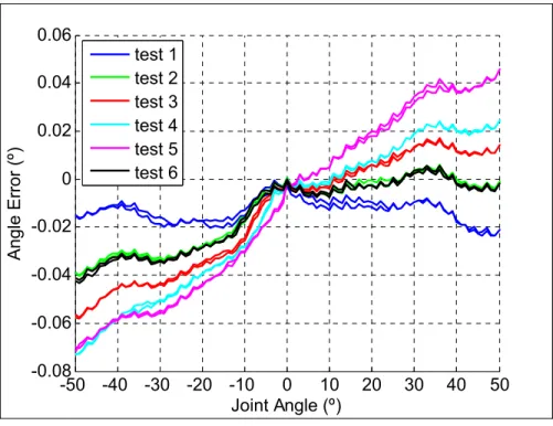
4.2 Detailed analysis of joint 6 ... 46

4.3 Detailed analysis of the 2nd axis ... 48

4.3.1 Effect of the tool weight ... 48

4.3.2 Robot arm stiffness effect ... 51

CHAPTER 5 ERROR MODELS ... 53

5.1 Nominal direct kinematics ... 53

5.2 Axis 6 model ... 55

5.3 Stiffness model ... 57

5.4 Direct kinematic models ... 61

5.4.1 Nominal model ... 61

5.4.2 11-parameter model ... 61

5.4.4 Kinematic calibration ... 62

CHAPTER 6 INVERSE KINEMATICS ... 65

6.1 Nominal inverse kinematics ... 65

6.1.1 Finding q1, q2 and q3 ... 65

6.1.2 Case with C=0 ... 67

6.1.3 Case with C≠0 ... 67

6.1.4 Finding q4, q5 and q6 ... 69

6.1.5 Wrist singularity (q5=0) ... 70

6.2 Iterative inverse calculation ... 71

CHAPTER 7 CALIBRATION METHODS ... 75

7.1 Procedure for taking measurements ... 75

7.2 Points needed for calibration ... 77

7.3 Calibration procedure ... 79

7.4 Verification procedure ... 80

7.5 Error vs. iterations ... 81

7.6 Expected error vs. real position error ... 83

7.7 Verification results ... 84

7.7.1 Results from nominal kinematics model ... 85

7.7.2 Results from entire kinematic calibration model ... 86

(11)

XI

7.7.4 Results found for 34-parameter calibrations from 80 to 200

measurements ... 99

7.7.5 Worst random 34-parameter procedures from 80, 120, 180 and 200 measurements ... 102

CONCLUSION ...109

ANNEX I POSITION REPEATABILITY OF THE ABB IRB 1600-6/1.45 ...113

ANNEX II FARO ION LASER TRACKER ACCURACY ...117

ANNEX III FARO ION LASER TRACKER REPEATABILITY ...121

ANNEX IV FARO ION LASER TRACKER 24-HOUR TEST ...123

ANNEX V ABB IRB 1600-6/1.45 POSITION STABILIZATION TIME ...127

ANNEX VI CIRCLE PATH ACCURACY TESTS WITH A TELESCOPIC BALLBAR ...129

(12)

(13)

LIST OF TABLES

Page

Table 3.1 xyz coordinates of the 9 targets (CAD + real points) ...40

Table 4.1 Range of motion for each joint ...45

Table 4.2 Tests for 6th_{axis analysis ...46}

Table 4.3 Maximum TCP errors ...51

Table 4.4 Tests for stiffness analysis ...51

Table 5.1 Nominal DHM parameters for the ABB IRB 1600 robot ...54

Table 5.2 Coefficients of the Fourier fit ...56

Table 5.3 Nominal robot model ...61

Table 5.4 Robot model for 11 parameters ...62

Table 5.6 Full robot kinematic model ...63

Table 6.1 Stabilization of the iterative inverse kinematics ...74

Table 7.1 Expected position error for the nominal kinematic model for 8 targets. ...86

Table 7.2 Expected position error for the kinematic calibration model (3 kg). ...86

Table 7.3 Expected position error for the kinematic model (6 kg). ...87

Table 7.4 Position errors for a 34-parameter calibration from 200 identification measurements (3 kg) ...89

(14)

XIV

Table 7.8 ISO 9283 position and orientation errors for the four models (3 kg) ... 93

Table 7.9 Position and orientation errors found for the four models (3 kg) ... 95

Table 7.10 Relative position errors (from virtual frame, 3 kg) ... 98

Table 7.11 Relative position errors (from 3 targets, 3 kg) ... 99

Table 7.12 Position and orientation errors for the 34-parameter procedures (3 kg) . 100 Table 7.13 Worst expected errors from pose measurements for the 34-parameter procedures (3 kg) ... 103

Table 7.14 Position statistics for the five 34-parameter procedures chosen (6 kg) .. 104

Table 7.15 Position statistics reduced to the 6th axis for the five 34-parameter procedures (3 kg) ... 105

(15)

LIST OF FIGURES

Page

Figure 3.1 Axis-by-axis rotation for identification ...26

Figure 3.2 Placing frame i ...28

Figure 3.3 Position of the nominal and real robot base frame ...32

Figure 3.4 Three points that determine the base frame ...33

Figure 3.5 End-effector used for holding the nine SMRs ...35

Figure 3.6 Identifying 5th and 6th axes ...36

Figure 3.7 Placing the 6th frame ...37

Figure 3.8 Geometry to find the 6th frame ...38

Figure 4.1 The IRB 1600 robot of which the positioning performance was analyzed using a Faro laser tracker ...43

Figure 4.2 Axis error analysis ...44

Figure 4.3 Position and angular errors at the TCP when moving each joint one by one ...45

Figure 4.4 Position representation for each of the five tests. ...47

Figure 4.5 Joint 6 angle errors ...47

Figure 4.6 Moving axis 2 to evaluate stiffness ...48

Figure 4.7 Picture of the real measurement points ...49

Figure 4.8 Stiffness effect with fully extended arm and a payload of 1.8 kg ...50

Figure 4.9 Stiffness effect with fully extended arm and a payload of 4.8 kg ...50

Figure 4.10 Equivalent θ2 error ...52

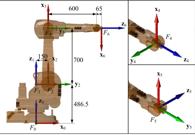
Figure 5.1 Frames corresponding to the DHM notation for the ABB IRB 1600 robot ...55

(16)

XVI

Figure 5.3 Robot arm representation ... 57

Figure 5.4 Estimating ΔL ... 58

Figure 5.5 Equivalent θ2 error ... 60

Figure 5.6 Equivalent θ2 error for a different combination of parameters ... 60

Figure 6.1 Solutions for q3 ... 68

Figure 6.2 Block diagram of the algorithm ... 72

Figure 6.3 Iterative inverse kinematics representation for iteration i ... 72

Figure 7.1 Random ISO cube points (left) and all range points (right) with respect to the robot and laser tracker. ... 79

Figure 7.2 Evolution of calibration step ... 82

Figure 7.3 Analysis of the expected error ... 83

Figure 7.4 Position error in ISO cube area (3 kg) ... 91

Figure 7.5 Position error in all robot range area (3 kg) ... 91

Figure 7.6 Position error in ISO cube area (6 kg) ... 92

Figure 7.7 Position error in all robot range area (6 kg) ... 92

Figure 7.8 ISO 9283 position errors reduced to the 6th axis (3 kg) ... 94

Figure 7.9 ISO 9283 orientation errors (3 kg) ... 94

Figure 7.10 Position errors reduced to the 6th_{axis for the four models (3 kg) ... 96}

Figure 7.11 Orientation errors for the four models (3 kg) ... 96

Figure 7.12 Position of the 434 sphere points chosen for relative analysis ... 97

Figure 7.13 Relative position errors from a virtual frame (3 kg) ... 98

Figure 7.14 Relative position errors from 3 targets (3 kg) ... 99

Figure 7.15 Position errors reduced to the 6th axis for the four 34-parameter procedures (3 kg) ... 101

(17)

XVII

Figure 7.17 Position errors for the five 34-parameter procedures chosen (6 kg) ...104 Figure 7.18 Position errors reduced to the 6th axis for the five 34-parameter

procedures (3 kg) ...106 Figure 7.19 Orientation errors for the five 34-parameter procedures (3 kg) ...106

(18)

(19)

LIST OF ABBREVIATIONS AND ACTONYMS CPC Complete and parametrically continuous

DH Denavit-Hartenberg

DHM Denavit-Hartenberg modified, as defined in (Craig, 1986)

DBB Double-ball bar

DOF Degree of freedom

TCP Tool center point

SMR Spherically-mounted reflector s(θ) sin(θ)

c(θ) cos(θ) si sin(qi)

ci cos(qi)

Trans(x,y,z) Geometrical translation {x,y,z}

Rot(v,θ) Geometrical rotation of θ around unit vector v

RMS Root mean square

(20)

(21)

LIST OF SYMBOLS AND UNITS OF MEASUREMENT kg Kilogram g Gram N Newton Hz Herz (measures/second) s Second ms Millisecond

º Degree (“deg” is used in some figures) rad Radian

m Meter mm Millimeter µm Micrometer

Nm Newton-meter (torque)

(22)

(23)

INTRODUCTION

Nowadays, two measures are commonly used for describing the positioning performance of industrial robots: repeatability and accuracy.

Loosely speaking, pose repeatability is the ability of a robot to repeatedly return to the same pose. In robotics, repeatability, as defined in ISO 9283 and used by all industrial robot manufacturers, actually refers to unidirectional repeatability only, i.e., the ability to return to the same pose from the same direction, thus minimizing the effect of backlash. Multidirectional repeatability can be twice the unidirectional repeatability or even worse.

Repeatability can be improved by either using direct-drive motors (as in some SCARA robots), high-precision gear trains (as in most Staübli robots) or by placing high-resolution encoders at the output of the gear trains. All of these solutions, however, considerably raise the manufacturing cost of an industrial robot.

Loosely speaking, volumetric (also called absolute) accuracy is the ability of the robot to attain a command pose with respect to a fixed reference frame. Since identifying such a reference frame is not always simple, accuracy is most typically tested in relative measurements, e.g., distance accuracy is the ability of the robot to displace its tool center point (TCP) a prescribed distance.

Accuracy is obviously affected by the same factors as multidirectional repeatability; actually it is lower bounded by the multidirectional repeatability of the robot. Accuracy is influenced mostly by geometric inaccuracies and elasticity, present in both the links and the transmissions. Fortunately, these two types of errors can be modeled to some extent in a process known as robot calibration (Abderrahim et al., 2007).

The demand for industrial robots having better repeatability and higher volumetric accuracy has been constantly growing in the past decade, especially in the aerospace sector (Summers,

(24)

2

2005). Today, most industrial robot manufacturers and a few service providers (such as Dynalog in the USA) offer robot calibration services. Furthermore, most industrial manufacturers now adopt the ISO 9283 norm, which was not the case a decade ago (Greenway, 2000; Schröer, 1999). Nevertheless, the only upfront information regarding the positioning performance of an industrial robot continues to be a single measure specified as “positioning performance according to ISO 9283”, which actually refers to the average unidirectional position repeatability and accuracy at five poses obtained from thirty cycles. A few additional performance measures might sometimes be obtained from the robot manufacturer (e.g., found in the product manual of the robot), such as linear path

repeatability and linear path accuracy, but even this information is highly insufficient and

impossible to use for comparison purposes.

The absolute accuracy of a given robot is virtually never specified by its manufacturer. The accuracy of a robot is not important as long as poses of the robot end-effector are manually taught. In this case we only want the robot to be repeatable. However, in offline programming the accuracy becomes an important issue since positions are defined in a virtual space from an absolute or relative coordinate system. There are also some industrial applications where a robot is used as a measurement system; in this case, the accuracy of the robot is the accuracy of the measurement system.

Improvement of the robot accuracy requires a study of the direct kinematic model. Using the nominal kinematic model of a robot and adding error parameters we can find a mathematical model that represents the robot better than the nominal kinematic model. This improved model must reduce position and orientation errors, i.e., improve the robot accuracy.

In this thesis, we propose different mathematical models which take into account different combinations of error parameters to represent the positioning behavior of the robot. These calibration methods are applied and tested on an ABB IRB 1600-6/1.45 industrial robot using a Faro laser tracker. The main objective of this project is to improve the accuracy of our robot.

(25)

3

As summarized by (Andrew Liou et al., 1993; Karan and Vukobratovic, 1994) there are five factors that cause robot errors: environmental (such as temperature or the warm-up process), parametric (for example, kinematic parameter variation due to manufacturing and assembly errors, influence of dynamic parameters, friction and other nonlinearities, including hysteresis and backlash), measurement (resolution and discretisation of joint position sensors), computational (computer round-off and steady-state control errors) and application (such as installation errors).

Although robot calibration has been studied for more than two decades, the theory remains quite the same as in the early 1980s (Barker, 1983). What is different nowadays is that robots are built better (i.e., their repeatability is greater) and the sources of errors (with respect to their nominal models) are somewhat different. Measurement equipment is also better, i.e., more accurate, though certainly not much more affordable. The mathematical models that used to work for robots a decade or two ago are no longer optimal for today’s robots. Furthermore, the accuracy required today in some potential robot applications is much higher than a decade ago.

Robot calibration can be divided into several categories and subcategories: absolute and relative calibration, open-loop and closed loop calibration, with or without feedback, etc.

1. Absolute vs. relative calibration

An absolute calibration takes into account where the robot base is placed whereas a relative calibration disregards the actual location of the robot base. In other words, if we want more than one robot to share the same coordinate system they need to be “absolute” calibrated to agree with the same “absolute” reference frame (also called world frame). A relative calibration is of interest when we are positioning the robot relatively to a local frame (also called object or user frame), so we need a tool, such as a touch probe, which allows us to locate objects in the robot working space. An absolute calibration needs six more parameters than a relative calibration because we need to represent the relative frame with respect to an absolute frame.

(26)

4

2. Open-loop vs. closed-loop calibration

Whenever we use a measurement system to directly measure the pose of the robot tool, such as a laser tracker, we apply an open-loop calibration. We can find several methods used for measuring robot position as the measuring technology has improved a lot in the past two decades.

Some examples of open-loop methods are acoustic sensors (Stone and Sanderson, 1987), visual systems such as cameras (Meng and Zhuang, 2001; Puskorius and Feldkamp, 1987), coordinate measuring machines (CMM) (Driels et al., 1993; Lightcap et al., 2008; Mooring and Padavala, 1989) and, of course, laser tracking systems (Shirinzadeh, 1998). There has also been some research work that allows a laser tracking system to identify the 6 parameters of the tool pose (Vincze et al., 1994).

On the other hand, a closed-loop method is used if the robot tool is constrained to lie on a reference object of precisely known geometry. This method only needs a switch such as a touch probe to detect the contact with an obstacle. When the robot is placed at the contact position the joint values given by the encoders are registered.

One example of closed-loop calibration is the MasterCal commercial product from American Robot, where the constraints are the diameter of two spheres and the distance between their centers. Other examples are the use of planar constraints (Ikits and Hollerbach, 1997), or point constraints (Meggiolaro et al., 2000) or (Houde, 2006).

3. Thesis organisation

This project is organized into seven chapters. Chapter 1 presents a literature review on robot calibration. Chapter 2 defines the project objectives and methodology. Chapter 3 describes a preliminary kinematic robot calibration performed by moving each axis individually. It also presents the theory of the full kinematic calibration making reference to the work done before using Sklar’s method (Mooring et al, 1991, p. 177). Once the robot is calibrated, we need to

(27)

5

set the base frame and the tool frame to establish a relationship with the external world. Chapter 3 also specifies how to establish an arbitrary and/or absolute base and proposes two tool calibrations: one in case we do not know the end-effector’s geometry and another in case we perfectly know this geometry (e.g., by measuring the end-effector on a CMM).

Chapter 4 discusses the axis-by-axis tests performed to the robot. These tests are based on axis identification and angle offset analysis for each joint of the robot, i.e., level 2 calibration. In this chapter, we find that the 6th axis has a peculiar non-linear behavior and that the robot arm weight is high enough to affect the linearity of axes 2 and 3.

Chapter 5 describes the kinematic and non-kinematic error models proposed in this thesis. We show how the compliances of axes 2 and 3 are modeled and how the motion pattern of axis 6 is fitted to a second order Fourier function.

Chapter 6 shows the nominal inverse kinematics and a slightly novel method to iteratively find the inverse kinematic solution of a fully calibrated and generic 6-revolute-axes serial robot.

In Chapter 7 we show all tests we performed to reach satisfactory calibration results. We describe a generic calibration procedure which corresponds to 120 measurements detailing the measurement acquisition, calibration method and verification tests.

(28)

(29)

CHAPTER 1 LITERATURE REVIEW

In this chapter we describe the generic calibration methods established in the literature, more precisely the robot calibration process, the three levels of robot calibration, the kinematic representation used for calibrated robots and the optimization methods used for parameter identification. We also mention the most relevant commercial solutions for robot calibration and some recent robot calibration results reported in literature.

The kinematic representation allows modeling the robot with parameters that define the geometry of the robot. Once we obtain a model to represent the behavior of the robot it is necessary to find a way to calculate the inverse kinematics for a given pose.

1.1 Robot calibration process

A typical robot calibration process consists of four sequential steps (Roth et al, 1987): modeling, measurement, identification and correction. The modeling step consists of representing the real robot through its direct kinematics equations. It is the mathematical model that takes into account the various error parameters. Data from the real robot allows generating the equations that the identification algorithm will use to find an improved robot model, better than the nominal kinematic model.

We could divide a full and complete robot calibration solution in three main steps: tool calibration, robot calibration and inverse kinematics computation.

1.2 Tool calibration

We may usually calibrate the tool at the same time as the robot is being calibrated. However, a separate tool calibration must be taken into account when the tool which we want to be precisely positioned is not the one that we use during calibration.

(30)

8

1.3 Robot calibration

By robot calibration researchers usually mean finding a new direct kinematics model that can represent the real robot better than the nominal model. The nominal model is the one used in the robot controller, and for robots with so-called inline wrists (the axes 4, 5 and 6 intersect at one point), the inverse kinematics of the nominal model are relatively simple and can be solved analytically. A robot calibration implies error parameters inserted to design parameters (nominal model) that represent the real source of errors. These parameters are called error parameters which must be found by the calibration method.

Although optimization algorithms are not primordial when calibrating a robot they can be very helpful improving precision if they are used appropriately. Some optimization algorithms are described in Section 1.6.

A robot calibration can be divided into three levels. The calibration method will be defined depending on which real error factor it represents and how many error parameters it uses. As explained in (Mooring et al., 1991), there are three levels of robot calibration.

1.3.1 Level-1 models

A level-1 calibration is also known as a “joint level” calibration. The purpose is to correctly define the relationship between the desired joint position (θd) and the real joint position (θr).

In a nominal model we consider θr=θd, but in real life we have a complex relationship

f ( )

r d

θ = θ . This relationship may be difficult to find but we can reach good approximations with linear functions. The most basic one would be:

1 0

r k d k

θ = θ + (1.1)

(31)

9

1.3.2 Level-2 models

A level-2 calibration is defined as the entire robot kinematic calibration. That means that some (or all) of the geometric design parameters are changed. Distance and angle offsets are added as error parameters to the robot’s nominal design. At the same time, a level-2 model can include a level-1 model to calibrate the joints.

When an entire kinematic calibration is needed we can identify the robot’s joint axes and extract the kinematic parameters placing frames that relate each joint axis with the next one. The calibration needs the “virtual” joint axes all in the same absolute reference frame and the geometry of the tool (end-effector) referred to the robot’s tool frame. To extract the virtual axes we must set all robot joints at 0º, and each joint has to be moved one by one taking measures by intervals (Mooring et al, 1991, p. 177). A circle that minimizes the sum of error squares can fit these points. From this circle we can extract the axis.

This idea was developed independently by several researchers. Once we have the virtual robot axes there are two basic methods to extract the kinematic parameters: Stone’s method and Sklar’s method (Mooring et al, 1991, p. 177). Stone’s method (Stone., 1986) finds the kinematic model known as “S-model” (6 parameters per joint) and Sklar’s method finds the DH representation of the robot placing the frames at the appropriate place. Both methods are explained and compared in (Mooring et al., 1991).

1.3.3 Level-3 models

The level-3 calibration takes into account the non-geometrical error sources. Non-geometrical sources of errors can be stiffness, friction, backlash, dynamical parameters, etc. Level-3 calibration is usually combined with a level-2 and level-1 calibration. Most common robot calibrations include a full kinematic calibration (level-2) and sometimes a few parameters describing the stiffness of the robot’s arm (level-3).

(32)

10

1.4 Kinematic modeling

For a nominal kinematic modeling, the best-known four-parameter representation is the one given by Denavit-Hartenberg (Denavit and Hartenberg, 1955). This so-called DH notation is widely used in robotics.

There is also a very similar and well-known representation commonly referred to as Denavit-Hartenberg Modified (DHM) notation which is the notation defined by Craig (1986). The main difference between the last two representation methods remains on the order of the geometrical transformations. Both make a translation and rotation over the X and Z axis (one translation and one rotation each). The DH notation starts with the X axis while the DHM notation starts with the Z axis (translation and rotation around the same axis can be alternated with no final effect). For a detailed review of the direct kinematic modeling, see (Craig, 1986; Paul, 1981; Slotine and Asada, 1992).

The DH notation has been used by several researchers for robot calibration, such as Wu (1984) or Ma et al. (1994). However, this representation introduces singularity problems when two consecutive axes are parallel or almost parallel (Hayati, 1983). The CPC model eliminates this problem (Zhuang and Roth, 1992) by representing the relationship between each link with three translations and one rotation instead of two translations and two rotations.

Other types of representations have also been used. There is five-parameter representation for prismatic joints (Hayati and Mirmirani, 1985) or even six parameter representation (Stone., 1986), but if we insert more than four parameters the calibration problem becomes redundant.

1.5 Inverse kinematics computation

We should normally describe how we are going to solve the inverse kinematics of the calibrated robot. There are many inverse kinematics solutions but not all of them are suitable

(33)

11

to all robot calibration methods. Depending on which type of calibration we use we will need one or another inverse kinematics solution. Inverse kinematics calculation can be divided in two main types: algebraic and iterative.

1.5.1 Algebraic

We should usually try to find an algebraic solution from our direct kinematics model. However, as we add error parameters to our basic kinematic model, the simplifications that we can usually do on a nominal model can no longer be done.

1.5.2 Iterative

When an algebraic solution cannot be found, an iterative method must be applied. This numerical method approaches to the solution at each iteration. Industrial robots often have path motion planners that divide a trajectory into a large quantity of points, and inverse kinematics must be applied to each point of the path.

Any of the optimization methods previously described for robot calibration could be used, however, better optimization methods exist as the problem is more specific. In the worst case we have to find as many parameters as the number of joints that the robot has.

The iterative (or numerical) methods can be divided into two types (Chen and Parker, 1994; Wang and Chen, 1991): (1) Newton-Raphson and predictor-corrector-type algorithms, and (2) optimization techniques by formulating a scalar cost function.

Examples of the first type can be found in (Angeles, 1985) who uses Newton-Raphson method and in (Goldenberg et al., 1987) or (Tsai and Orin, 1987) who use a predictor-corrector-type algorithm. The problems of these methods appear when the Jacobian matrix is singular.

(34)

12

Examples of the second type can be found in (Chen and Parker, 1994; Goldenberg et al., 1987; Goldenberg and Lawrence, 1985; Wang and Chen, 1991). These predictor-corrector-type algorithms are numerically more stable since the Jacobian matrix is not used.

1.6 Optimization algorithms

Once we have defined a model (kinematic or non-kinematic) we must find the error parameters by measures taken from the real robot. The optimization algorithm which is suitable for most types of robot calibration is nonlinear and unconstrained. Different methods and algorithms have been developed, such as the CPC error model (Complete and Parametrically Continuous). It establishes an error model with a minimum number of parameters (Motta and McMaster, 1999; Zhuang and Roth, 1992).

Plenty of algorithms, more precisely the genetic algorithm (Wang, 2009), represent small variations of direct kinematic parameters and the end-effector error is represented by a fitness function. At every generation, a population of parameters is created and brings a better solution to replace the existing solution. This technique does not need complex calculations like the inverse of the Jacobian matrix.

Other alternatives for robot calibration have been tested, like Taguchi method (Karan and Vukobratovic, 1994) or (Judd and Knasinski, 2002). The work (Zhuang and Roth, 2002), for example, uses different methods (similar to the CPC model) to identify the unknown parameters.

All optimization methods can be mainly classified into two types: line-search methods and trust-region methods. We can also mention an optimization method that differs from the first two types: the Nelder-Mead method.

(35)

13

1.6.1 Line-search methods

There are various line-search methods. They differ by the way they compute the line search direction. We can find the following line-search methods: Newton’s method, gradient descent method and Quasi-Newton method (Bonnans and Lemaréchal, 2006).

Newton’s method is also known as Newton-Raphson method. Newton algorithms are implemented in Matlab’s optimization toolbox in the functions fsolve, fminunc and lsqcurvefit.

1.6.2 Trust-region method

The trust-region method is also known as restricted step method. It handles the case when the Jacobian matrix is singular and is useful when the initial guess is far from a local minimum. This method approximates the objective function with a simpler function in the neighborhood of the solution at each iteration.

Trust region methods are dual to line search methods. The first one chooses a step size before a search direction while the second one chooses a search direction and then a step size.

1.6.3 Nelder-Mead

This optimization algorithm was proposed by John Nelder and Roger Mead (Nelder and Mead, 1965). It is also called simplex method (a non linear method that is different from the known linear simplex method). It evaluates the objective function over a polytope in the parameter space. If we have two parameters, the polytope is a triangle as we are in a 2D plane. If there are n-dimensions, we have an (n+1)-sided polytope.

The algorithm compares these n+1 points and deletes the worst one. The worst point is replaced by its reflection through the remaining points in the polytope. This algorithm is

(36)

14

simple and does not need gradient information but it takes time to achieve a solution when we have more than six variables. This method is also implemented in Matlab’s optimization toolbox, in the function fminsearch.

1.7 Commercial solutions for robot calibration

Most robot manufacturers offer calibration as an option. For example, in the case of ABB Robotics, most (but not all) of its robots can be calibrated at the factory with the CalibWare software for about C$2,000, using a Leica laser tracker, a single SMR (Spherically-mounted reflector) and around 40 error parameters. However, ABB does not offer an on-site calibration service, unlike KUKA. ABB also has a tool to improve resolver offsets due to motor exchange and maintenance: the calibration pendulum.

As an example, L-3 MAS Canada at Mirabel use Motoman industrial robots and have them calibrated on-site by Motoman, who use a third-party calibration software (from Dynalog). Similarly, Messier-Dowty at Mirabel use three KUKA industrial robots and have them calibrated on-site by KUKA.

1.7.1 Dynalog

Dynalog is a Detroit-based privately held company founded in 1990 by Dr. Pierre De Smet, then professor at Wayne State University. Dynalog is by far the most renowned expert in robot calibration. While the company offers several products improving the accuracy of industrial robots, the two of greatest interest are the CompuGauge hardware and the DynaCal software. The first is a 3D (x, y ,z) measurement device based on four string encoders that intersect at one point. Dynalog claims that the volumetric accuracy of the CompuGauge measurement device is 0.150 mm and its repeatability is 0.020 mm inside a cubic working volume of side 1.5 m. The price of this device is at least US$9,000, but while not expensive, the device is quite bulky and difficult to install.

(37)

15

DynaCal is software for robot calibration that accepts measurement data from the CompuGauge device or from any other precision 3D or 6D measurement device. The software and here adapters for fixing SMRs are sold to industry for more than US$40,000. While all demonstrations of DynaCal show the use of a laser tracker and a single SMR, it seems that DynaCal can also work with three SMRs, thus calibrating the complete pose of the end-effector.

Dynalog also has a specific patented product to calibrate robots that is going to be used for piece inspections (De Smet, 2001). Dynalog offers a complete robot library which makes it possible to calibrate any robot from any brand.

1.7.2 Nikon Metrology

Metris International Holding was purchased by Nikon in 2009 to create Nikon Metrology. Metris, a market leader for CMM based laser scanning, was founded in 1995 and is headquartered in Belgium. In 2005, Metris acquired Belgium-based Krypton, which was specializing in robot calibration since 1989.

Nikon Metrology offers a large number of metrology systems, but the two that are of particular interest to us are the K-Series Optical CMM and the ROCAL software. The first one is basically a three-camera system that measures the spatial coordinates of up to 256 infrared LEDs (thus, it can provide 6D measurements). The volumetric accuracy of the K-Series Optical CMM is better than 0.090 mm which is close to the laser tracker accuracy and certainly sufficient for robot calibration. Its price is about C$80,000.

ROCAL is software for robot calibration, very similar to Dynalog’s DynaCal. It seems that some of the differences are a better integration with some robot brands (KUKA, Mitsubishi and COMAU) and the software’s incompatibility with measurement devices other than the K-Series Optical CMM. The software also relies on complete pose measurement data.

(38)

16

1.7.3 Teconsult

Teconsult is a Germany based university spin-off offering a unique 3D optional measurement device called ROSY and the robot calibration software that goes with it. Teconsult was founded by Prof. Lukas Beyer in 1999. ROSY is a measuring tool based on a videometric principle with two digital CCD cameras. Two cameras are used in order to get a more uniform volumetric accuracy. The tool is attached to the robot flange and is used to measure, with respect to the robot flange frame, the spatial position of the center of a small white ceramic ball that is fixed with respect to the robot’s base. The ROSY device itself is calibrated on a CMM before shipment.

The calibration procedure consists of reorienting the tool and measuring the position of the ball for 40 different poses (Beyer and Wulfsberg, 2004), for a single location of the ceramic ball. According to reference (Beyer and Wulfsberg, 2004) the volumetric accuracy of ROSY is ±0.020 mm inside a spherical measurement range of ±2 mm. However, ROSY is offered in several different sizes, and there is no information whether that volumetric accuracy is for a small or for a large ROSY device.

ROSY is rather bulky and requires removal of the end-effector from the robot. Furthermore, it requires several relatively thick cables to be run along the robot arm. A complete ROSY system for tool, base and robot calibration is about €17,500 (US$21,000). However, it seems that Teconsult does not offer any means to calculate the inverse kinematics.

1.7.4 Wiest AG

Wiest is another Germany based university spin-off offering another unique 3D optical measurement device called LaserLAB and the robot calibration software that goes with it. Wiest AG was founded by Dr. Ulrich Wiest who has been working in the field of robot calibration since 1996 (he obtained his doctoral degree in 2001).

(39)

17

LaserLAB is patent-pending (Wiest, 2003) and consists of five small-range one-dimensional laser distance sensors mounted to a common frame and with their lasers intersecting at a common point. A ball is attached to the end-effector of the robot while the LaserLAB device is stationary. By measuring the five distances to the ball (when the center of the ball is approximately at the lasers intersecting point), the spatial coordinate of the center of the ball with respect to the LaserLAB are determined. The repeatability of the LaserLAB is ±0.020 mm, while its volumetric accuracy is better than ±0.100 mm (typically ±0.035 mm), inside a measurement range of 39.5 mm × 38.5 mm × 36.5 mm.

One disadvantage of the LaserLAB is the high likelihood of the sphere colliding with the measurement device while the robot is re-oriented. Furthermore, the only way to measure with a wide range of robot configurations is to use extension rods of different lengths at the end of which a sphere is mounted, rendering that solution practically inconvenient and therefore realistically inaccurate.

1.7.5 American Robot Corporation

American Robot Corporation (ARC) is a US company based in Pittsburg, Pennsylvania. ARC was established in 1982 and is a manufacturer of industrial robot controllers, industrial robots, and automation systems. It has three major product lines, the Universal Robot Controller, the Merlin articulated six axis robot, and the Gantry 3000 modular gantry robot. ARC also offers a robot calibration software called MasterCal, which makes use of a standard touch probe attached to the flange of a robot and two fixed precision balls separated by a precisely known distance.

The MasterCal calibration procedure was invented and patented by Mr. Wally Hoppe (Hoppe, 2008), a Group Leader and Senior Research Engineer at the University of Dayton Research Institute in Ohio, USA. The basic concept for Mr. Hoppe’s calibration method is an extension of (Meggiolaro et al., 2000), where a single ball-in-socket mechanism was used. Mr. Hoppe’s institution had a huge military contract for robot inspection of aircraft engines

(40)

18

and this is how he ended up devising a robot calibration method (he no longer works in robotics). In the course of the patent application, he eventually came across some inventions that are pretty close to this one, although he worked with his lawyer to demonstrate that they do not infringe. The closest method to his invention is by ABB (Snell, 1997). That method uses a single large-diameter precision ball of known diameter and a touch probe. Another very close invention is (Knoll and Kovacs, 2001), which is very general and does not give a lot of detail.

1.8 Recent calibration results reported in the literature

Recent research has been mainly focused on level-2 and level-3 calibrations. An example of a level-3 calibration using a stiffness model is (Lightcap et al., 2008), that applies a torsional spring model to represent the flexibility of the harmonic drives by physically meaningful parameters, this model takes into account the flexibility caused by the end-effector. The model improves the mean / maximum values from 1.77 mm / 4.0 mm to 0.55 mm / 0.92 mm for a Mitsubishi PA10-6CE when loaded at 44 N (validated with only ten measurements on a CMM). This method is more simple than the one proposed in (Khalil and Besnard, 2002) as it does not need the computation of the generalized Jacobian. Also (Caenen and Angue, 1990) represented the angular deformation caused by gravity force. A similar method exists dealing with joint angle dependent errors (Jang et al., 2001).

An example of kinematic calibration is given in (Ye et al., 2006), where an absolute calibration was performed to an IRB 2400/L with a Faro Xi laser tracker. The mean position error is reduced from 0.963 mm to 0.470 mm for twenty measurements (maximum values are not given, the area of calibration is not given either).

Another example of absolute calibration with a laser tracker is (Newman et al., 2000). Using a Motoman P8 robot, the 27 error parameters from their kinematic model are identified by measuring 367 targets moving each axis separately. The kinematic model that gave best results (for a validation of 21 measurements) corresponds to a “circle-point” algorithm that improves the RMS error from 3.595 mm to 2.524 mm.

(41)

19

We can finally mention the work performed by (Bai et al., 2003) that uses a modified CPC model (MCPC) (Zhuang et al., 1993) to improve the kinematics of a PUMA 560 with 30 error parameters and a laser tracker measure system. Using 25 measures for parameter identification and 15 measures for verification they reach a mean position error of 0.1 mm, however, when they use a CMM they find that the same position error is 0.4-0.5 mm. The CPC model avoids the singularities associated with parallel axes.

Other examples of stiffness kinematic models that do not use meaningful parameters are (Jang et al., 2001; Meggiolaro et al., 2005). As explained by Lightcap et al. (2008), it is better to use meaningful parameters to be able to extrapolate to unknown charges.

In the IRB 1600 product documentation, it is stated that the typical mean/maximum positioning accuracy is 0.300 /0.650 mm. We know from Dr. Torgny Brogardh, that this is validated for one tool target (apparently the same target used for calibration). However, we do not have more information regarding the validation procedure, such as the number of measurement poses.

(42)

(43)

CHAPTER 2

OBJECTIVES AND METHODOLOGY

This section describes the objectives of this project and the methodology followed.

2.1 Thesis objectives

The main objective of this project is to establish a robust and efficient calibration method for our ABB IRB 1600 industrial robot. Another objective is to investigate and compare the performance of several level-1, level-2 and level-3 calibration methods. No dynamic calibration will be taken into account.

The calibration methods proposed will be compared to the nominal model, which will include the calibration of the robot base and the end-effector. The calibration of the base is taken into account in the nominal model since we are not able to measure the robot base, so the results are more favorable for the robot manufacturer. The calibration of the tool is also taken into account since we do not have the exact measures of the tool with respect to the tool flange of the robot.

Once the robot parameters are identified, we need to modify the original desired targets (poses) into so-called “fake” targets. To do so, we need to use an iterative inverse kinematics algorithm based on the new direct robot model to calculate the corrected joint values for the desired end-effector pose.

Once we have an improved model of the robot and the procedure to generate the fake targets is established, we will be able to validate our model. To validate our models we are going to use a large number of measures in contrast to other researchers. Many researchers and companies usually use from 50 to 100 measures to find a calibrated model and no more than 50 measures to validate the model found. In this case it is not possible to have a good

(44)

22

estimation of the maximum error value found with the new model. However, we will use about 1000 measures to validate our models.

We will also validate our models with at least three points from the tool (most validation tests will be performed with eight tool-point measurements). So if we improve the position error of at least three tool-points (which are not in the same line), this will mean that we also improve the orientation errors. In addition, tests for evaluating the improvement of the orientation errors will also be performed.

2.2 Methodology

All calibration models will be tested with an ABB IRB 1600-6/1.45 robot and using a Faro ION laser tracker as a measurement system. They are both controlled by a PC running Matlab and an Ethernet local area network (LAN).

A laser tracker is relatively simple to use and can quasi-continuously (typically every millisecond) measure the position of a single SMR or even measure the complete pose in static mode (by measuring the positions of three SMRs, however, using ADM only), in the entire workspace of an industrial robot. Unfortunately, laser trackers are excessively expensive ($100K or more) and very sensitive to air turbulences. Furthermore, their volumetric accuracy and repeatability is much worse than that of two high-precision single-axis measurement instruments commonly used for machine tool calibration: the laser interferometer system and the telescoping bar. These are, however, not described in the ISO guide and are rarely used in conjunction with industrial robots.

The mathematic representation chosen to model the kinematics of the robot is the one defined by Craig (Craig, 1986) and also known as the DHM notation (Denavit Hartenberg Modified). Using the methods explained by Mooring et al (1991, p. 177) and adapting the kinematic parameter extraction to the DHM notation we can find the kinematic model of a robot. In addition we consider some additional error parameters representing the behavior of the 6th

(45)

23

An end-effector was manufactured to hold nine spherically-mounted reflectors (SMRs). This end-effector allows a wide range of poses in which at least one (or three) SMR are visible by the laser tracker. The weight of this end-effector is 3 kg (holding all SMRs). Extra weight can be added by up to eight steel discs (each disc weights 375 g), so the maximum end-effector weight is 6 kg.

(46)

(47)

CHAPTER 3

KINEMATIC CALIBRATION

This chapter describes the first step of our robot calibration study, namely, what we can loosely refer to as preliminary robot calibration. Basically, we directly identify each of the six robot axes by rotating the joints one by one.

The base frame should normally be measured directly, by measuring the mounting pattern on the bottom of the robot’s base. However, once the robot is installed, this can only be done if the robot was mounted using the guide holes on a precise base plate with, for example, three tooling balls (the location of the centers of which are precisely known with respect to the robot’s base mounting pattern). In our case, and in most industrial installations, such a precise mounting base plate is not used. Similarly, yet this is much simpler, the geometry of the tool can be measured exactly on a CMM (i.e., the location of the TCP with respect to the flange reference frame, i.e., tool0 for an ABB robot). However, this is not always done in practice. Hence, we find the optimal base and tool reference frames through two separate calibration processes.

Finally, when the kinematic parameters (concerning the base, the robot geometry and the tool) have been found, we can add other error parameters that do not correspond to geometric errors, as explained in Chapter 5.

3.1 Kinematic parameter extraction from identified joint axes

A complete and full kinematic calibration is explained, which neither needs special computer power nor iterations to minimize an error function. The procedure is similar to other procedures explained by Mooring et al. (1991, p.177), who made an extraction of kinematic parameter from joint axes for a DH model (Sklar method) and for an S-model (Stone method). The calibration needs the “virtual” joint axes all in the same absolute reference and the dimensions of the used tool referred to the robot’s tool frame.

(48)

26

If the errors in the real robot were due only to kinematic errors, with this entire kinematic calibration we can extract the real geometric links of the robot obtaining an error equivalent to the noise measurement. That’s what we found by simulating the method explained in this chapter. In simulation, if the measurement noise is forced to zero, the position error is zero.

3.1.1 Method to find the axis of each joint

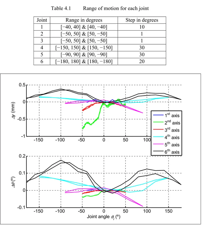
Starting from the home configuration in which all robot joints are at 0º, each joint has to be moved one by one in equal increments, each time measuring the position of the TCP. A circle that minimizes the sum of all error squares can be fitted to these points for each axis. From this circle we can extract the robot axis.

axis 1 (-40º, 0º, 40º) axis 2 (-40º, 0º, 40º) axis 3 (-40º, 0º, 40º)

axis 4 (-40º, 0º, 40º) axis 5 (-40º, 0º, 40º) axis 6 (-40º, 0º, 40º) Figure 3.1 Axis-by-axis rotation for identification

(49)

27

Although we need to fit a number of points in 3D space to a circle, for which many algorithms exist, they all require an initial estimate for the center and the plane of that circle. This initial estimate can be obtained analytically from any three points, ideally equally distanced along the circle.

Let the coordinates of three points P1, P2, and P3, be denoted by the vectors p1, p2, and p3,

respectively. Also let the unit vector that is normal to the plane (that contains these three points) be denoted by vaxis:

(

)

(

)

(

1 2

) (

3 2

)

axis 1 2 3 2 − × − = − × − p p p p v p p p p (3.1)

It can be easily shown that the coordinates x, y, and z, of the center of the circle are the solution of the following system of linear equations (representing three planes passing through the center of the circle, the first also passing through all three points, the second also normal to line p1p2 and the third also normal to p3p2):

1 2 3 det 0 1 1 1 1 c   =       p p p p (3.2)

(

1 2

)

2 2 1 1 2 T T T 0 c − + − = p p p p p p p (3.3)

(

3 2

)

2 2 3 3 2 T T T 0 c − + − = p p p p p p p (3.4)

where pc=[x,y,z]T. A different solution is explained in (Schneider and Eberly, 2003, Section

13-10).

Once the initial estimate for vaxis and pc is found, we can use the Gauss-Newton least-squares

fitting method (Gander et al., 1994).

3.1.2 Placing the link frames

Once we find the axes of all joints, the next step is to place the frame of each joint i with the information of the axis i and the axis i+1. All frames must be referenced to the same absolute

(50)

28

coordinate system, which can be the base frame of the measure system (a particular case for the robot’s base and for parallel axis is explained below).

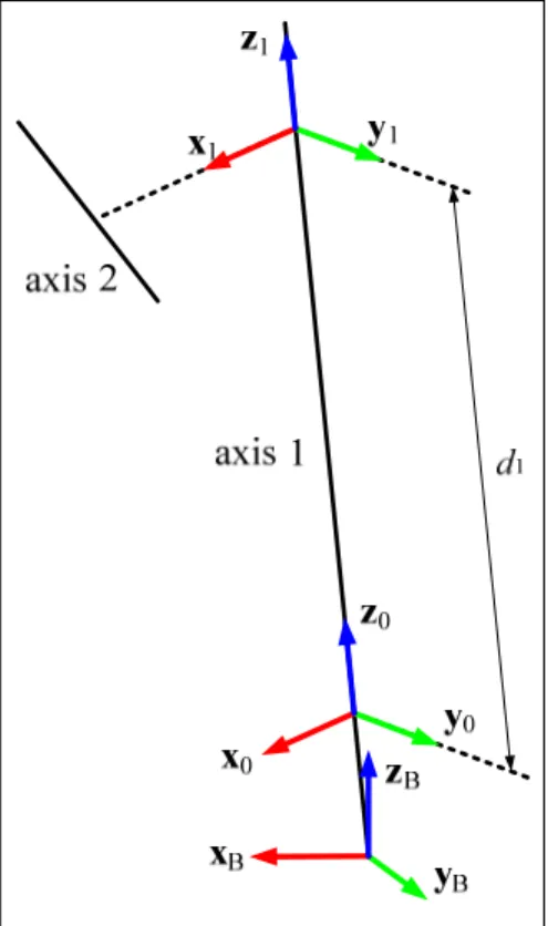
To make all transformations suitable to a DHM representation we will use the information between two consecutive axes (like the common normal line, its distance or the angle between two axes). Figure 3.2 shows two consecutive axes and the common normal line that connects them (dotted line). To place the frame i we must follow next steps if a DHM notation is used.

Figure 3.2 Placing frame i

We will always place first the vector zi in the direction of the ith axis. The origin is at the

intersection between the ith axis and the common normal line (or the intersection of both axes if they intersect). The component xi is found by x_i = ×z z , which corresponds to the _i _i₊₁

common normal vector if the two axis are not coincident. Finally, we have that y_i = ×z x . _i _i

In this way it is possible to make a DHM representation suitable between two consecutive frames. This happens because only with a translation and rotation around the common normal line (vector xi) we can make the transformation from zi to zi+1. After that, it is

possible to make a rotation and translation around the zi+1 axis to place the origin, xi+1 and

(51)

29

However, a DHM representation will not be possible from an arbitrary base frame F0 because

its z vector will never be perfectly perpendicular to the base plane xy (F0 has its z vector in

the same direction as the first axis, see Section 3.2).

3.1.3 Dealing with parallel axes

When we have two parallel axes we can use a threshold tolerance to consider those axes parallel or not. In other words, two axes will never be parallel because there is an alignment angle error. If this error is considerable we can use the method described before to place the frames.

If the alignment error is very small it is possible to force both axes to be parallel. That means that the center point of each axis is kept but we apply the same direction for both of axes. In this case, the center is the origin of the new frame.

In the case where the alignment error is very small but we do not force the axes to be parallel, if we use the DHM model, a small variation of parameters can result into big kinematic changes. In this case it is important to take into account that the CPC model can be more suitable than the DH or DHM models since this problem is attenuated.

3.1.4 Error parameters needed for a full calibration

As described before, all link transformations can suit a DHM representation except for the first one, which needs two extra error parameters if we consider an arbitrary base. So we have six parameters for the first joint and four parameters for the other five joints which make 26 error parameters to determine. If we want a relative calibration we can skip the first six parameters of the base frame.

(52)

30

Finding those parameters is direct once we have identified the axes of the robot, finding the axes may take a few seconds if there are a lot of points that define each axis. No computational power is needed and the solution can be obtained directly.

We mentioned that 26 parameters are required to complete the robot calibration. However, in this robot calibration the end-effector is represented by a DHM transformation, so only two parameters are taken into account for the position of the TCP relative to the end-effector due to the kinematic representation chosen (which only takes into account 4 parameters per link). In this case, if we want to consider the TCP as part of the calibration process we must add one error parameter (because to define a position with respect to a frame we need 3 parameters). Summarizing, a total of 27 error parameters are needed for a complete kinematic calibration for the position the TCP with respect to an arbitrary base. This corresponds to the minimality justification from Bernhardt and Albright (1993, p.163).

3.1.5 Homogeneous transformation

Sometimes we will need to represent a homogeneous transformation in its six descriptive parameters. A 4×4 homogeneous transformation matrix can hold up to six parameters. Here we show one method to extract these six parameters. This transformation is represented by a translation along the xi, yi and zi axes followed by rotations about the xi, yi and zi axes

consecutively:

(

) (

) ( )

Trans , , Rot , Rot , Rot ,

j i = x y zi i i αi βi γi A x y z , (3.5)

( ) ( ) ( )

c( )c( ) c( )s( ) s( ) s s c c( )s( ) s s s c( )c( ) s( )c( ) c s c s( )s( ) c s s s( )c( ) c( )c( ) 0 0 0 1 i i i i i i i i i i i i i i i i i i i j i i i i i i i i i i i i i i x y z β γ β γ β α β γ α γ α β γ α γ α β α β γ α γ α β γ α γ α β −    ₊ ₋ ₊ ₋    =_ _ − + +     A . (3.6)

It is possible to extract the original parameters {xi, yi, zi, αi, βi, γi} if we have the generic Aij

(53)

31

obtained proceeding with next steps, imposing the cosine positive for βi to obtain values

closer to zero:

(

2

)

1,3 atan2 j , 1 sin ( j) i i i β = A + − A (3.7)

Once we obtain , and are completely defined:

( )

2,3 3,3 atan2 , cos( ) cos j j i i i i i α β β  −  = _ _   A A (3.8) 1,2 1,1 atan2 , cos( ) cos( ) j j i i i i i γ β β  ₋  = _ _   A A (3.9)

Obviously, this generic representation can suit a DHM representation but not vice versa.

3.2 Base frame definition

In robotics, the xy base plane is placed perpendicularly to the first axis (z0 is placed along the

first robot axis). This plane will never be exactly the same as the “tangible” reference plane (the plane of the base mount) since we are looking for a geometrical error. Consider Figure 3.3, where the first frame F1 is placed as explained before and errors are exaggerated.

The definition of the base is important if we want to calibrate the robot for a specific, physical and measurable frame (see the comparison between an absolute and a relative calibration in the introduction). We could call FB the real base frame (composed by {xB, yB,

zB}) and F0 the nominal base frame (composed by {x0, y0, z0}). The first one is tangible but

the second one is not. It is possible to find the second one by the information of the first and second axes and the nominal parameters.

(54)

32

Figure 3.3 Position of the nominal and real robot base frame

In the case where we consider the base frame as the “official” tangible base frame, provided by the manufacturer, F0 and FB should be very close. If the first and second axis were exactly

in its nominal position (so there are no errors for the first and second axis), frames F0 and FB

(nominal and real robot base frame respectively) would be exactly the same. The real base frame FB is found by measurements on the robot base plane (which is the same as xByB

plane) and has the origin on the intersection of this plane with the first axis line. zB is

perpendicular to the robot’s real floor plane and xB and yB can be placed arbitrarily on the

floor plane.

The nominal base frame F0 is found by a translation along −z1 of the nominal distance d1

from the F1 frame (no error parameters are included in this step):

1= 0 Trans(0,0, )d1

F F (3.10)

(55)

33 0 0 = B B F H F (3.11) 0 B ≅I4 H (3.12) Ideally, 0 B

H should be equal to the identity matrix. However, with errors it can hold up to six parameters for a geometrical transformation. If our base frame definition is important (in other words, if the link between FB and F0 is important) we must use those six parameters.

Otherwise, we have six parameters to place this FB frame wherever we want or we can force

those six error parameters to be zero (then, F0 and FB are coincident).

To have an idea, if we consider that the robot base is the nominal base F0 for the ABB IRB

1600-6/1.45 robot, we find a maximum position error of 2.1 mm for 337 measurements. However, if we consider that the real robot base FB has its origin placed at the intersection of

the tangible robot base plane xy with the 1st axis, zB perpendicular to this plane and xB

through the projection of x0 to the floor plane, we get errors up to 15 mm for the same 337

measures.

3.3 Finding the base from three points

Usually we will not be able to measure the exact position of the robot’s base. We must find some characteristic points on the floor plane where the robot is placed. We describe here one method to find the origin pB and xB, yB, zB axis of the robot base from the 3 points shown in

Figure 3.4.

(56)

34

These three points are:

1. The first one on the axis ±xB.

2. The second one on the axis ±xB, this one must be on the direction of +xB in comparison to

the first point.

3. The third one on the axis +yB.

From the figure we can obtain xB, yB, zB :

2 = 2− 1 v p p (3.13) 3 = −3 1 v p p (3.14) 2 B 2 = v x v (3.15) 2 3 B 2 3 × = × v v v v z (3.16) B = ×B B y z x (3.17)

Finally, to find the origin pB we can project the point p3 on the line p1+tv2 (Schneider and

Eberly, 2003):

(

)

2 0 2 T 1 T 3 2 t = v p −p v v (3.18) B = +1 t0 2 p p v (3.19) 3.4 End-effector calibration

An end-effector was manufactured to hold all of our nine spherically-mounted reflectors (SMRs), namely five 1.5-inch and four 0.5-inch SMRs. This end-effector increases the range of poses in which at least three SMRs are visible by the laser tracker, thus allowing measurements of the complete pose of the robot end-effector.