Universit´e de Montr´eal
Multi-Prover and Parallel Repetition in Non-Classical Interactive Games
par Tommy Payette
D´epartement d’informatique et de recherche op´erationelle Facult´e des arts et des sciences
M´emoire pr´esent´e `a la Facult´e des arts et des sciences en vue de l’obtention du grade de Maˆıtre `es sciences (M.Sc.)
en informatique
Aoˆut 2009
c
Universit´e de Montr´eal Facult´e des arts et des sciences
Ce m´emoire intitul´e:
Multi-Prover and Parallel Repetition in Non-Classical Interactive Games
pr´esent´e par: Tommy Payette
a ´et´e ´evalu´e par un jury compos´e des personnes suivantes: Alain Tapp pr´esident-rapporteur Louis Salvail directeur de recherche Gilles Brassard codirecteur Geˇna Hahn membre du jury
R´
esum´
e
Depuis l’introduction de la m´ecanique quantique, plusieurs myst`eres de la nature ont trouv´e leurs explications. De plus en plus, les concepts de la m´ecanique quantique se sont entremˆel´es avec d’autres de la th´eorie de la complexit´e du calcul. De nouvelles id´ees et solutions ont ´et´e d´ecouvertes et ´elabor´ees dans le but de r´esoudre ces probl`emes informatiques. En particulier, la m´ecanique quantique a secou´e plusieurs preuves de s´ecurit´e de protocoles classiques.
Dans ce m´emoire, nous faisons un ´etalage de r´esultats r´ecents de l’implication de la m´ecanique quantique sur la complexit´e du calcul, et cela plus pr´ecis´ement dans le cas de classes avec interaction. Nous pr´esentons ces travaux de recherches avec la nomenclature des jeux `a information imparfaite avec coop´eration. Nous exposons les diff´erences entre les th´eories classiques, quantiques et non-signalantes et les d´emontrons par l’exemple du jeu `a cycle impair. Nous centralisons notre attention autour de deux grands th`emes : l’effet sur un jeu de l’ajout de joueurs et de la r´ep´etition parall`ele. Nous observons que l’effet de ces modifications a des cons´equences tr`es diff´erentes en fonction de la th´eorie physique consid´er´ee.
Mots cl´es: preuves int´eractives `a plusieurs prouveurs, jeux du cycle impair, nonlocalit´e, complexit´e du calcul quantique, intrication.
Abstract
Since the introduction of quantum mechanics, many mysteries of nature have found explanations. Many quantum-mechanical concepts have merged with the field of computational complexity theory. New ideas and solutions have been put forward to solve computational problems. In particular, quantum mechanics has struck down many security proofs of classical protocols.
In this thesis, we survey recent results regarding the implication of quantum mechanics to computational complexity and more precisely to classes with inter-action. We present the work done in the framework of cooperative games with imperfect information. We give some differences between classical, quantum and no-signaling theories and apply them to the specific example of Odd Cycle Games. We center our attention on two different themes: the effect on a game of adding more players and of parallel repetition. We observe that depending of the physical theory considered, the consequences of these changes is very different.
Keywords: multi-prover interactive proofs, Odd Cycle Games, non-locality, quantum computational complexity, entanglement.
Contents
R´esum´e i
Abstract iii
Contents iv
List of Symbols and Abbreviations vii
List of Figures viii
Acknowledgements ix
1 Introduction 1
1.1 Incompleteness of Classical Theory . . . 1
1.2 Related Works . . . 2
1.3 Contribution . . . 3
1.4 Structure of the Thesis . . . 3
2 Quantum Information 5 2.1 The Qubits . . . 5
2.2 Systems of Qubits and their Evolution . . . 6
2.3 The Trace Function . . . 8
2.4 Measurements . . . 9
2.5 Entanglement . . . 12
3 Computational Complexity Theory 15 3.1 Definitions and Non-Interactive Classes . . . 15
3.2 Interaction with a Single Prover . . . 17
3.3 Interaction with Many Provers . . . 20 iv
CONTENTS v
3.4 Interaction with Entanglement . . . 22
4 Two-prover One-round Games 27 4.1 Games Parameters . . . 28
4.2 Strategies of the Provers . . . 28
4.3 Value of a Game . . . 30
4.4 Relationship with Complexity Theory . . . 32
4.5 Upper Bound for XOR Games . . . 33
4.6 Example: The Odd Cycle Game . . . 38
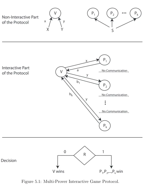
5 The Power of Many Provers 45 5.1 Many-Prover Classical Games . . . 46
5.2 Many-Prover Non-Classical Games . . . 48
5.3 Many-Prover Odd Cycle Games . . . 51
6 Parallel Repetition of Two-Prover One-Round Games 55 6.1 Parallel Repetition of Classical Games . . . 56
6.2 Parallel Repetition of Non-Classical Games . . . 60
6.3 Parallel Repetition of Odd Cycle Games . . . 66
7 Conclusion 73 7.1 Future Work . . . 74
Bibliography 75 A Mathematical Optimization 85 A.1 Optimization Problems . . . 85
A.1.1 Convex Optimization Problems . . . 86
A.1.2 Linear Optimization Problems . . . 87
A.2 Duality . . . 88
A.2.1 The Lagrange Dual Function . . . 88
A.2.2 Dual Problems . . . 89
List of Symbols
and Abbreviations
Abbreviation Description Definition
Z Set of natural number
R Set of real numbers
C Set of complex numbers
|ψ⟩ Quantum State page 5
I Identity matrix page 7
δ Kronecker delta function page 7
POVM Positive Operator-Valued Measure page 10
EPR Einstein-Podolsky-Rosen page 13
XOR Exclusive-OR page 23
List of Figures
3.1 Hierarchy of Complexity Classes. . . 18 3.2 Updated Hierarchy of Complexity Classes. . . 25 4.1 Two-Prover Interactive Game Protocol. . . 32 4.2 Impossibility of 2-Colourability of an Odd Cycle of Length 5. . . 39 5.1 Multi-Prover Interactive Game Protocol. . . 46 6.1 Two-Prover Interactive Game with Parallel Repetition. . . 56
Acknowledgements
I would like to thank my supervisors, Louis Salvail and Gilles Brassard, for their help and support. I would also like to thank my friends and my family for their encouragement, from which I found the motivation to complete this thesis.
Chapter 1
Introduction
Nowadays, information is a fundamental concept in computer science as well as in pure physics. Physicists and other scientists try to uncover the mys-teries behind nature using physical phenomena that can be explained, or at least approximated, to certain degrees with mathematical equations. At the same time, computer scientists work on a more abstract level to understand the amount of computational resources necessary to solve a problem. The two fields meet each other because any information system is implemented by physical means and is governed by a physical model. The link between physics and computer science is becoming even more important as computer components decrease in size. Indeed, at the limits of the nanometer scale, the choice of the physical model has a deep impact on the analysis of the computational resources. The most successful physical theory, quantum mechanics, has grown in popularity and has successfully explained many phenomena of nature.
1.1
Incompleteness of Classical Theory
It was proven in 1964 that a purely classical explanation of physical phenomena was incompatible with the predictions of quantum mechanics [Bel64]. At that time, some physicists thought that it was impossible for an event to have an effect instantaneously on another one. A local hidden theory is a theory that follows these lines of ideas. Another theory, quantum mechanics, allows in certain situation instantaneous correlations. It was proven in [Bel64] that predictions from quantum mechanics could
2 CHAPTER 1. INTRODUCTION
not be explained by local hidden theories.
This had many implications in the field of computational complexity theory since classification was made only with classical resources. When quantum mechanical concepts are taken into account, many classes of re-sources have to be redefined and new consequences emerge.
In this thesis, we present recent results about the differences of already established computational classes when non-classical physical resources are considered. We center our attention on classes with interaction and only to those with classical communication between the parties. To demonstrate the results, we use the framework of games, which are well suited for this type of classes. In particular, we survey how the addition of more players affects the outcome of a game and what consequences parallel repetition has on games.
1.2
Related Works
We are mainly interested in how quantum mechanics changes the setting of computational complexity classes with interaction, classical messages and cooperative provers. Other classes are described with different properties than the one we are interested. We give a brief summary of the related work.
There exist complexity classes for which interaction is done through a quantum channel: the class QIP (Quantum Interactive Proofs) [Wat03, KW00] and its multi-prover analogue, the class QMIP (Quantum Multi-prover Interactive Proofs)[KM02]. It has recently been shown [JJUW09] that QIP = PSPACE.
Other interactive complexity classes related to the subject include the classes RG (Referee Games) in the classical setting [Pap85, KM90] and QRG (Quantum Referee Games) in the quantum setting [Gut05, GW04, GW07]. In both of these classes, the provers are in competition with each other.
Some have studied zero-knowledge interactive classes in the classical set-ting [GMW91, GMR89] and in the quantum setset-ting [Wat02, Wat06, Kob07]. Finally, there are interesting results related to the hardness of approxi-mation of the value of games in [IKP+07, KRT07, KKM+08].
1.3. CONTRIBUTION 3
1.3
Contribution
The thesis describes many results and presents them in an organized manner to help the reader understand how the physical theory considered affects computational classification. It is not meant to be a comprehensive survey since this topic is still very active. However, results are chosen to indicate possible future lines of work, to the best of our knowledge. The contribution of the author is to group the research papers in a concise and organized manner through a unified notation for clear understanding.
1.4
Structure of the Thesis
The remainder of this thesis is divided into five chapters. Chapter 2 intro-duces the notions of quantum mechanics needed for this thesis. Chapter 3 introduces the notions of computational complexity theory and serves as a motivation for the study of games. Chapter 4 gives a description of the game framework. Chapters 5 and 6 are selections of results from recent papers. Chapter 5 presents results for multi-prover games and chapter 6, results on parallel repetition. Each of these chapters is divided into three sections: classical theory, non-classical theory and a section with a specific example.
Chapter 2
Quantum Information
The purpose of the present chapter is to introduce the reader to the notions of quantum information. This chapter is not intended to be a comprehensive introduction to the topic but rather presents essential tools of quantum information needed to understand this thesis. For more information on the topic, the reader is encouraged to consult [NC00]. Note that we assume that the reader is familiar with basic notions of linear algebra.
2.1
The Qubits
Like the classical bits, quantum bits, or qubits for short, are parts of a mathematical representation of a physical system. This abstraction is sim-ilar to the concept of states on and off in electronics for the underlying voltage measures they represent. There are many ways to construct the physical implementation to produce qubits but these techniques are beyond the scope of this thesis.
Analogously to the values 0 and 1 of a classical bit, a qubit can take values |0⟩ and |1⟩. Although classical bits are uniquely restricted to values 0 and 1, qubits can be in superposition of states |0⟩ and |1⟩ as in
|ψ⟩ = α|0⟩ + β|1⟩, (2.1)
where |ψ⟩ is used to describe the state and α and β are complex numbers with the restriction |α|2 +|β|2 = 1. Qubits can, therefore, be represented
in a two-dimensional complex vector space with orthonormal basis |0⟩ and |1⟩.
6 CHAPTER 2. QUANTUM INFORMATION
By the nature of quantum mechanics, it is not possible to measure di-rectly the values α and β to get a complete description of the state |ψ⟩. Rather, when a qubit is measured with respect to the orthonormal basis, the observation is 0 with probability |α|2 or 1 with probability |β|2.
2.2
Systems of Qubits and their Evolution
In general, the state of an n-qubit system can be represented in a 2n -dimensional vector space with complex inner product over C .
The standard notation in quantum mechanics is called the Dirac nota-tion. This notation represents a vector by |ψ⟩ where ψ is a label for the vector. In this formalism, the object|ψ⟩ is called a ket and the object ⟨ψ| is called a bra. The ket being a vector from a vector space, the bra is defined to be the conjugate transpose of the ket
⟨ψ| = ¯|ψ⟩T
=|ψ⟩†
where the dagger sign † indicates the conjugate transpose. We denote the inner and outer product between vector |φ⟩ and |ψ⟩ by ⟨φ|ψ⟩ and |φ⟩⟨ψ|, respectively. The name bra and ket have been taken from the definition of the inner product ⟨φ|ψ⟩ that is the bracket.
We describe a method to enlarge vector spaces. This is often erroneously called the tensor product but it should be really called the Kronecker prod-uct. The Kronecker product U ⊗ V of two matrices U and V of dimension M × M and N × N is calculated as follows. First, we write
u11V u12V . . . u1MV u21V u22V . . . u2MV .. . ... . .. ... uM 1V uM 2V . . . uM MV (2.2)
where uij is the element in the ith row and jth column of the matrix U .
Matrix (2.2) is a M × M matrix of N × N matrices. The final Kronecker product U ⊗ V is given by removing the parentheses for the matrices V in (2.2) producing an M N × MN matrix [Bra].
For notational convenience, when using the ket representation of vectors in Kronecker products, the symbol⊗ can be dropped. For example, we can write the Kronecker product of |0⟩ and |0⟩ by |0⟩ ⊗ |0⟩ = |0⟩|0⟩ = |00⟩.
It would be useless to describe the state of a physical system at a par-ticular time without being able to observe its evolution through time. In
2.2. SYSTEMS OF QUBITS AND THEIR EVOLUTION 7
fact, the evolution of a closed system can be described by transformations (unitary).
A transformation on a state can be represented either with matrix no-tation or by a set of linear transformations on the basis of this state. For example, transformations on qubits are represented by
U = [
u00 u01
u10 u11
]
or equivalently by the set of transformations |0⟩ U
7−→ u00|0⟩ + u10|1⟩
|1⟩ U
7−→ u01|0⟩ + u11|1⟩
where uij ∈ C with the condition that U is unitary.
Definition 2.2.1. [Unitary Transformations] A transformation U is said unitary if
U U† = I
where I is the identity matrix with the same dimensions as matrix U . Definition 2.2.1 is correct for finite Hilbert spaces. For infinite Hilbert spaces, we would also require U†U = I. Unitary transformations play an essential role in quantum mechanics. If the state of the system is |ψ⟩ at time t1 and |ψ′⟩ at time t2, then there exists a unitary transformation U
that relates the two closed states by
|ψ′⟩ = U|ψ⟩.
Note that quantum mechanics only indicate that the unitary transformation U exists; it does not indicate which unitary operator U it is.
It is worth mentioning at this point a very useful unitary transformation, the Hadamard transformation, defined by
H = √1 2 [ 1 1 1 −1 ]
and whose uses will be seen later.
In some cases, unitary transformations are not applied to the whole sys-tem. Take, for example, the case when the two qubits of a two-qubit system |ψ⟩ are physically separated. If a unitary transformation U is applied on
8 CHAPTER 2. QUANTUM INFORMATION
the second qubit only, the effect on the system is given by unitary trans-formation (I ⊗ U). In general for a two-qubit system, applying a unitary operation U1 on the first part of the system and U2 on the second part of
the system is equivalent to applying the unitary transformation U1⊗ U2 on
the whole system.
2.3
The Trace Function
A useful tool from linear algebra that will be used in this thesis is the trace function.
Definition 2.3.1 (Trace). The trace of a matrix A is defined to be the sum of its diagonal elements:
tr(A) =∑
i
Aii.
The trace has two important properties. For two matrices A and B whose products AB and BA exist, and a complex number z, the trace is linear
tr(zA + B) = ztr(A) + tr(B), and it satisfies
tr(AB) = tr(BA). (2.3)
For an operator A and a state|ψ⟩, it can be shown that property (2.3) of the trace implies
tr(A|ψ⟩⟨ψ|) = ⟨ψ|A|ψ⟩. (2.4)
For multi-qubit systems or systems of states, the trace can be taken only with respect to a certain qubit or state, this is called the partial trace. In this case, the qubit or the state in question is indicated as a subscript. Definition 2.3.2 (Partial Trace). Consider two states A and B with two vectors |a1⟩, |a2⟩ ∈ A and |b1⟩, |b2⟩ ∈ B from their appropriate state space
and a state described by ρ =|a1⟩⟨a2| ⊗ |b1⟩⟨b2|. Then the partial trace of ρ
with respect to B is given by
ρA= trB(ρ)
=|a1⟩⟨a2|tr (|b1⟩⟨b2|)
=|a1⟩⟨a2|⟨b1|b2⟩
where ρAis the reduced state of ρ on system A. The definition of the partial
2.4. MEASUREMENTS 9
2.4
Measurements
Now that we know that the state of a physical system can be represented by |ψ⟩ and its evolution in time by a unitary transformation U, we need to describe a mechanism to get information from a state. We obtain it by measuring the state but the information gained is dependent on the measurement made. Measurements are described by a collection {Mm} of
measurement operators living in the space of the state to be measured where the index m refers to the outcome of the measurement. The measurement operators are subject to the completeness equation
∑
m
Mm†Mm = I. (2.5)
If the system is in state |ψ⟩ immediately before measurement, then the probability that outcome m occurs after measurement is given by
Pr|ψ⟩[m] =⟨ψ|Mm†Mm|ψ⟩ = tr(Mm†Mm|ψ⟩⟨ψ|). (2.6)
The measurement changes the state of the system to |ψ′⟩ = √ Mm|ψ⟩
⟨ψ|M†
mMm|ψ⟩
Before giving an example of a measurement on a state, we define two important properties that an operator can have.
Definition 2.4.1 (Hermitian Operator). We say that an operator P is Hermitian if
P = P†. (2.7)
Definition 2.4.2 (Orthogonal Operator). We say that two operator Pm
and Pm′ are orthogonal if
PmPm′ = δm,m′Pm (2.8)
where δm,m′ is the Kronecker delta function defined by
δm,m′ =
{
1 if m = m′
0 if m̸= m′. (2.9)
To illustrate the effect of a measurement on a state, the example of the measurement of a qubit in the computational basis follows.
10 CHAPTER 2. QUANTUM INFORMATION
Recall that the state of the qubit can be given by equation|ψ⟩ = α|0⟩ + β|1⟩ (equation (2.1)) subject to |α|2 +|β|2 = 1. In the computational basis {|0⟩, |1⟩}, the outcomes m ∈ {0, 1} are obtained with measurement operators {M0, M1} defined by
M0 =|0⟩⟨0|,
and
M1 =|1⟩⟨1|.
Since M0 and M1 are Hermitian and M = M2, the probability of getting
measurement outcome 0 and 1 is given by
Pr|ψ⟩[m = 0] =⟨ψ|M0†M0|ψ⟩ = ⟨ψ|M0|ψ⟩ = |α|2,
and
Pr|ψ⟩[m = 1] =⟨ψ|M1†M1|ψ⟩ = ⟨ψ|M1|ψ⟩ = |β|2.
The state after outcomes 0 and 1 are obtained will be: |ψ′⟩ = M0|ψ⟩ |α| = α|0⟩ |α| , and |ψ′⟩ = M1|ψ⟩ |β| = β|1⟩ |β| ,
respectively. Since the statistics of the measurement of states α
|α||0⟩ and
|0⟩ and of states β
|β||1⟩ and |1⟩ are the same, the global phase factor can
effectively be ignored. After normalization, measuring a qubit in the state given by equation (2.1) with the computational basis {|0⟩, |1⟩} will lead to the final state
|ψ′⟩ = |0⟩ with probability Pr
|ψ⟩[m = 0] =|α|2,
and
|ψ′⟩ = |1⟩ with probability Pr
|ψ⟩[m = 1] =|β|2.
There are two cases of quantum measurements that are often seen in lit-erature: projective measurements and POVM (Positive Operator-Valued Measures). In some case, the use of these special cases simplifies the anal-ysis of a problem. Projective measurements with unitary transformations and auxiliary systems are POVM and POVM are equivalent to general mea-surements.
2.4. MEASUREMENTS 11
A projective measurement is described by an observable M that is a Hermitian operator with spectral decomposition
M =∑
m
mPm
where Pm is the projector onto the eigenspace of M with eigenvalue m.
The set of eigenvalues represents the set of possible outcomes. Similarly to general measurements, the outcome m occurs with probability
Pr|ψ⟩[m] =⟨ψ|Pm|ψ⟩
and after measurement, the state evolves to |ψ′⟩ = √Pm|ψ⟩
Pr|ψ⟩[m]
Being a special case of general measurements, projective measurements have an important property: the operators {Pm}M are orthogonal projectors.
This means that {Pm}M are Hermitian and orthogonal.
In order to describe an observable M , a complete set of orthogonal projectors {Pm}m is often given satisfying equations
∑
mPm = I as well as
equations (2.7) and (2.8). Moreover, when it is said to “measure in a basis {|m⟩}m”, this means to make the projective measurement with projectors
Pm =|m⟩⟨m|, where M =
∑
mmPm.
POVM are a particularly useful formalism. Let Mm be a measurement
operator such that ∑mMm†Mm = I describes a measurement on quantum
state |ψ⟩ and define
Em def
= Mm†Mm.
Then similarly to general measurements, {Em}m satisfies the completeness
relation (2.5). Each operator Em, also called POVM element, is sufficient to
determine the measurement outcomes and the set {Em}m is called POVM.
The practicality of the POVM formalism can be illustrated with a sim-ple examsim-ple. Suppose we are given one of two quantum states, |ψ1⟩ = |0⟩ or
|ψ2⟩ = (|0⟩+|1⟩)√2 , which are indistinguishable with perfect reliability but we
do not know which of the states it is. Although it is impossible to distin-guish the two states with perfect reliability, we can nonetheless devise an experiment that will distinguish the states some of the time and never make an error of mis-identification. Consider the POVM {E1, E2, E3} defined by
E1 =
√ 2
12 CHAPTER 2. QUANTUM INFORMATION E2 = √ 2 1 +√2 (|0⟩ − |1⟩)(⟨0| − ⟨1|) 2 , (2.11) E3 = I − E1− E2. (2.12)
These are clearly POVM since each operator is positive and satisfies the completeness relation (2.5). When we measure the state, we have that
⟨ψ1|E1|ψ1⟩ = 0, (2.13)
⟨ψ2|E2|ψ2⟩ = 0. (2.14)
By equation (2.6), equations (2.13) and (2.14) mean that the probability of measuring E1 and E2 from the state |ψ1⟩ and |ψ2⟩ respectively is 0.
Therefore, if the unknown state|ψ⟩ was indeed |ψ1⟩ there is zero probability
that E1 will be observed and if the state was |ψ2⟩ there is zero probability
that E2 will be observed. In other words, if the result of the experiment is
E2, the state was|ψ1⟩ and if the results is E1, the state was|ψ2⟩. When the
result is E3, it is impossible to know which state it was. In both cases, when
|ψ⟩ is |ψ1⟩ or |ψ2⟩, the probability of correctly identifying the unknown state
|ψ⟩ calculated from equation (2.6) is √1
2+2 ≈ 0.29. What is very interesting
from the standpoint of POVM is that this probability is higher than it would be possible with projective measurements. This example concludes the demonstration of how useful the POVM formalism is.
2.5
Entanglement
So far, we have explained how to represent the evolution of the state of a system, how to measure it and what information can be extracted as well as how the measure changes the state of the system. This section presents one of the most puzzling concepts in quantum mechanics: entanglement.
Consider a composite system of m + n qubits described by the state |ψ⟩. If |ψ⟩ can be written as |ψ⟩ = |ψ1⟩|ψ2⟩ with two separate states |ψ1⟩
and |ψ2⟩ of m and n qubits respectively, then it is called a product state.
If the state cannot be separated in this manner, we say the state |ψ⟩ is entangled. Entangled states play a crucial role in quantum information and it is probably the most astonishing phenomenon in quantum mechanics.
Well-known examples of entangled states in the literature are the two-qubit Bell states:
|Φ+⟩ = √1
2.5. ENTANGLEMENT 13 |Φ−⟩ = √1 2(|00⟩ − |11⟩), |Ψ+⟩ = √1 2(|01⟩ + |10⟩), |Ψ−⟩ = √1 2(|01⟩ − |10⟩),
where the last state is also called the Einstein-Podolsky-Rosen (EPR) pair, introduced in [EPR35].
To get a better understanding of the power of entanglement, an example will be used. Suppose Alice and Bob are separated and share an EPR pair where Alice keeps the first qubit and Bob keeps the second qubit. Suppose now that Alice measures her qubit. With probability 1
2, she will get the
outcome 0 and with probability 12, she will get the outcome 1. By the nature of the EPR pair, Alice then knows that Bob will get measurement outcome 1 or 0 with perfect probability before he measures. However, from the perspective of Bob, who does not know if Alice has measured yet or not, his state is still the EPR pair. Only if Alice tells him the result she got, will he know that his state is in fact |0⟩ (if Alice got outcome 1) or |1⟩ (of Alice got outcome 0). The troubling effect is that no matter who measured first, they will still get opposite outcomes.
You might think that when Alice measures her state a signal is sent to the state of Bob. But experiments indicate that if this is the case, it would be supraluminal and would violate special relativity. In [Bra], a paradoxical scenario is described that indicates how signalling theory is problematic:
[...]if the two particles are moving away from one another, rela-tivity allows for a paradoxical situation in which each particle is measured after the other in its own space-time frame, and there-fore it does not even make sense to say that the first-measured particle “decides” the outcome for both particles: neither par-ticle is measured first! This whole concept revolted Einstein to such an extent that he called it “spooky action at a distance”. Another explanation of the strange phenomenon might be that quantum mechanics is wrong and that each particle is already determined to be in the state |01⟩ or |10⟩ before Bob and Alice receive it. That is, randomness occurs before separation. Again in [Bra], an experiment that was made is described in which each participant Bob and Alice apply the Hadamard transformation upon receiving their state. For details of the experiment,
14 CHAPTER 2. QUANTUM INFORMATION
consult [Bra]. It is shown that the resulting statistical outcomes would be different in the case that the state would be already |01⟩ or |10⟩ and the case that the state is changed at measurement. Experiments have shown that the state is in fact changed after measurement and not at the separa-tion[FC72,ADR82,AGR82,TBG+98,TBZ+98].
All these results do not prove that quantum mechanics is correct but rather that a na¨ıve classical interpretation is not sufficient. Can there be another classical explanation? This question puzzled Einstein, Podolsky and Rosen but it was not until 1964, that Bell’s theorem ruled out any classical theory [Bel64].
Chapter 3
Computational Complexity
Theory
This chapter gives motivations for the study of games in chapter 4. The notion of games that will be presented in this thesis is linked to the notion of multi-prover interactive proofs in computational complexity. This is the reason we devote an entire chapter to this topic.
A short reminder of relevant complexity classes will be presented. We assume the reader is familiar with basic notions of complexity theory. For more details on the topic, consult [Sip06] for an introduction to complexity theory and [Wat] for more information on complexity theory classes with quantum information.
3.1
Definitions and Non-Interactive Classes
Computational complexity theory is the science that studies the amount of resources required by an algorithm to solve a given computational prob-lem. Common resources include time and space with respect to the size of the input, but also randomness, alternations, interaction and many more. The theory of computational complexity characterizes quantified amount of resources into computational classes.
Central elements in computational complexity theory are languages. A language is a set of strings (e.g.:{000110,1010}) over an alphabet Σ (e.g.:Σ1 = {0, 1}). In this setting, we can study the problem of
decid-ing whether of not a given strdecid-ing is in a language. An important set of 15
16 CHAPTER 3. COMPUTATIONAL COMPLEXITY THEORY
problems are decision problems: problems for which the solution is either yes or no. A particular set of decision problems, promise problems, are well suited for the game setting of the next chapter. A promise problem is a decision problem for which the input is a subset of all possible string Σ∗. We formalize the notion of promise problems with the following definition from [Wat].
Definition 3.1.1 (Promise Problems). A promise problem is a pair A = (Ayes, Ano) where Ayes, Ano ⊆ Σ∗ are sets of strings satisfying Ayes∩Ano =∅.
The sets Ayes and Ano are sets of yes-instances and no-instances having
answers yes and no respectively.
Adding the condition Ayes∪ Ano = Σ∗ to the definition of promise
prob-lems gives the definition of a language. We can group any probprob-lems, and in particular promise problems, of related complexity into classes. In the remaining of this section we will give the description of different complexity classes with respect to promise problems rather than just languages. The motivation for this transition will be clear in the next chapter.
In complexity theory, we are also interested by relations between differ-ent classes. If there exists a function f so that for all x∈ Ayes, f (x)∈ Byes
and for all x ∈ Ano, f (x) ∈ Bno then we say there is a reduction from the
class A to B, A≤ B. If there is as well a reduction from class B to A, B ≤ A, we say that the two classes are equivalent. There are some restrictions for the type of functions for this to be true, but for the results presented you can assume the function f is a classical polynomial-time function on inputs in Ayes∪ Ano.
In the literature, classes of problems are described in terms of languages and not on promise problems. In this thesis however, we will follow non-standard definitions based on the promises problems. We give the definition of some classes with which the reader should be familiar.
Two of the most discussed classes are the class P and NP. Their defini-tion with respect to promise problems is given [Wat].
Definition 3.1.2 (Class P ). A promise problem A = (Ayes, Ano) is in
P if and only if there exists a deterministic Turing machine M in time polynomial in the length of the input |x| that accepts every string x ∈ Ayes
and rejects every string x∈ Ano.
Definition 3.1.3 (Class N P ). A promise problem A = (Ayes, Ano) is in
NP if and only if there exists a polynomially bounded function p(|x|) and a deterministic Turing machine M in time polynomial in the length of the
3.2. INTERACTION WITH A SINGLE PROVER 17
input|x| with the following properties. For every string x ∈ Ayes, M accepts
(x, y) for some y ∈ Σp(|x|), and for every string x∈ Ano, M rejects (x, y) for
all strings y ∈ Σp(|x|).
Nowadays, the list of classes is very large. Many results in complexity theory put in relation one class to another or prove the equivalence of two classes. We give the definition of three more fundamental classes: PSPACE, EXP and NEXP.
Definition 3.1.4 (Class SPACE ). A promise problem A = (Ayes, Ano) is
in PSPACE if and only if there exists a deterministic Turing machine M running in space polynomial in |x| that accepts every string x ∈ Ayes and
rejects every string x ∈ Ano.
Definition 3.1.5 (Class EXP ). A promise problem A = (Ayes, Ano) is in
EXP if and only if there exists an deterministic Turing machine M in time exponential in the length of the input |x| (meaning time bounded by 2p(|x|), for some polynomial-bounded function p(|x|)), that accepts every string x∈ Ayes and rejects every string x∈ Ano.
Definition 3.1.6 (Class NEXP ). A promise problem A = (Ayes, Ano) is in
NEXP if and only if there exists a polynomially bounded function p(|x|) and a deterministic Turing machine M in exponential time in the length of the input |x| with the following properties. For every string x ∈ Ayes, M
accepts (x, y) for some y ∈ Σ2p(|x|), and for every string x∈ A
no, M rejects
(x, y) for all strings y ∈ Σ2p(|x|).
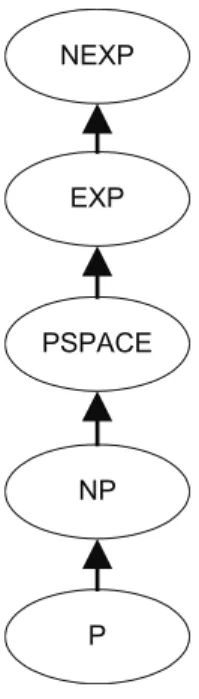
Note that we do not introduce the class NPSPACE for nondetermin-istic polynomial space since it was shown that PSPACE = NPSPACE in [Sav70]. Therefore, nondeterminism does not add more power to the class PSPACE. Figure (3.1) puts in relation the complexity classes described so far by drawing the more powerful complexity classes higher. Lines indi-cate containments; for example, NP contains P. Note that none of these containments are known to be strict.
Next, we give a brief overview of other classes along with some results that are going to be relevant to the rest of the thesis.
3.2
Interaction with a Single Prover
Introduced in [GMR85], an interactive proof system is a model of compu-tation in which a polynomial number of messages are exchanged between
18 CHAPTER 3. COMPUTATIONAL COMPLEXITY THEORY EXP NP PSPACE P NEXP
Figure 3.1: Hierarchy of Complexity Classes.
two parties: a prover and a verifier. We let the prover have unbounded computational power and the verifier be polynomial time but allowed to use randomness. The goal of the prover is to convince the verifier about the truth of a statement that might be beyond the reach of the verifier. The verifier wants to challenge the prover in order to verify his assertion. To do so, the verifier sends a question q ∈ Q to the prover for which the prover answers a ∈ A where Q and A are sets of possible questions and answers of polynomial size. A round of interaction is defined as a question from the verifier and an answer from the prover. After a certain number of rounds, based on the answers he received, the verifier either accepts or rejects the statement of the prover. If the answer is a member of the yes-instances Ayes, the verifier should accept it and if the answer is from the no-instances
Ano, the verifier should reject it.
Sometimes, the verifier cannot be convinced without doubt of the truth of the statement using a polynomial number of messages. This is why we introduce the completeness and soundness probabilities. In the formalism of promise problems, if x ∈ Ayes, the completeness probability is the
prob-ability that the verifier accepts it, that it does not reject a true statement. If a x ∈ Ano, the soundness probability is the probability that the verifier
accepts it, that he accepts a false statement. Formally, we define these two notions for interactive proofs with promise problems in the following
3.2. INTERACTION WITH A SINGLE PROVER 19
definitions.
Definition 3.2.1 (Completeness). Given a promise problem A = (Ayes, Ano), the completeness probability c is the minimum probability for
which the verifier V accepts any x∈ Ayes
Pr[V accepts x]≥ c. (3.1)
Definition 3.2.2 (Soundness). Given a promise problem A = (Ayes, Ano),
the soundness probability s is the maximum probability for which the veri-fier V accepts x∈ Ano
Pr[V accepts x]≤ s. (3.2)
We define the class BPP again with the non-standard promise problems formalism.
Definition 3.2.3 (Class BPP ). A promise problem A = (Ayes, Ano) is in
BPP (Bounded-error, Probabilistic, Polynomial time) if and only if there exists a probabilistic Turing machine M in time polynomial in the length of the input |x| with completeness probability 23 and soundness probability 13. The interactive proof system described above with the verifier given the power of the class BPP characterizes the class IP.
Definition 3.2.4 (Class IP ). A promise problem A = (Ayes, Ano) is in IP
(Interactive Proofs) if and only if there exists an interactive proof system for A given that the verifier has the power of the class BPP and the prover has unbounded computational power. The communication between the verifier and the prover remains classical.
Historically, some complexity theorists wanted to increase the power of the class NP by introducing interaction. It turns out that if the verifier is bounded by the class P only (without randomness), the resulting interactive class would be equal to the class NP [AB]. Therefore, having the power of NP with interaction does not add more power to the class. On the other hands, by letting the verifier be probabilistic as in the class BPP, it was shown that the class IP =PSPACE in [Sha92], which might increase the power of the class beyond NP and BPP if NP ̸= PSPACE. It was also shown by non trivial arguments that restricting the completeness probability to be 1 does not change the power of the class. However, restricting the soundness probability to be 0 reduces the power of the class IP to the class NP because the verifier becomes deterministic [AB].
20 CHAPTER 3. COMPUTATIONAL COMPLEXITY THEORY
To illustrate the concept of the class IP, an illustrative scenario borrowed and adapted from [AB] is presented. Suppose that Alice has a friend Bob who claims that he can distinguish the taste of two similar soda drink Cole and Petsi. To verify that assertion, Alice is going to prepare one cup of each drink labelled 1 and 2 in the absence of Bob and then present them to him. If after tasting them, Bob can correctly identify each one, Alice is more convinced that Bob is telling the truth. The promise in this case is that exactly one of the bottle of Alice contains Cole and exactly one contains Petsi. The query (two cups) from Alice and the answer of Bob constitute one round of interaction. However, Bob could give a random answer and with probability 12 give the right result. This is why Alice is encouraged to redo the test n times to increase her confidence level. At the end, Bob could have been lucky with probability only (12)n. Alice can choose the number n
of repetitions until she is satisfied and thus can detect a cheating Bob with probability 1− (12)n. Since Alice knows which cup has which soda drink, the completeness probability is 1 (i.e.: she will accept every good answer given by Bob). The probability that Bob will cheat successfully Alice, the soundness probability, is (12)n.
3.3
Interaction with Many Provers
Interactive proofs were generalized to more than one prover, resulting in the class MIP (Multiprover Interactive Proofs) in [BOGKW88]. Cryptographic purposes were originally the motivation behind this class. With this gen-eralization, all communication between any provers is forbidden as soon as interaction between provers and the verifier has started. However, since the provers are cooperative, they can initially agree on a shared strategy to convince the verifier. In the new paradigm, the verifier sends a question to each prover and makes his decision based on their answers. A round in multi-prover interactive proofs is a questions/answers tuple between the verifier and all provers.
Definition 3.3.1 (Class MIP ). A promise problem A = (Ayes, Ano) is in
MIP (Multi-prover Interactive Proofs) if and only if there exists a k-prover interactive proof system with k ≥ 2 for A, given that the verifier has the power of the class BPP and the provers have unbounded power. The com-munication between the verifier and the provers is classical and the provers cannot communicate once the interactive part of the protocol has started with the verifier.
3.3. INTERACTION WITH MANY PROVERS 21
For notational convention, MIPc,s[k, r] will be used to represent the class
of interactive proof systems with k-provers (k ≥ 2) and r-round (r ≥ 1) with completeness probability c and soundness probability s. We write simply MIP[k, r] when the specific values of c and s are not important and similarly. Similarly, we write MIP[k] when the value of r ≥ 2 is not important.
The original paper [BOGKW88] already demonstrated that increasing the number of provers to more than two does not change the power of the class, thus for any value k ≥ 2, MIP[k] = MIP[2]. It was further shown that NEXP = MIP[2, 1] [BFL90] and consequently that having more than one prover might increase the power of the class IP = PSPACE to MIP = NEXP (if PSPACE ̸= NEXP). After an increasing interest in two-prover one-round interactive proofs, several refinements [CCL90, Fei91, LS91] lead to the proof that every language in NEXP has a two-prover one-round interactive proof with perfect completeness and exponentially small soundness error [FL92]. Thus, the restriction of MIP1,s[2, 1] with
exponentially small soundness error s is as powerful as the more general MIP[k]. Later, the parallel repetition theorem for two-prover one-round interactive proofs appeared [Raz98].
To understand why more provers are more powerful than one prover, let’s revisit the experiment of distinguishing the taste of soda drinks Cole and Petsi. Let’s introduce another participant, Charlie, to the test. Now Charlie and Bob claim that they both can distinguish the taste of Cole and Petsi and want to convince Alice about that statement. Alice wants to make sure that BOTH participants tell the truth. She could do as before with each participant separately and detect each cheating participant with probability 1− (12)n after n repetition of the test. The probability that Alice detects
both participants if they cheat would then be (1− (12)n)2 because the two
events are independent of each other, enforced by the no-communication condition. In fact with two participants, to get the same probability as with one participant you just need to do more tests.
By looking at these results, one might think that two provers only affect the soundness of the experiment and by a right number of sequential rep-etitions it is possible to get the same results. If Alice does the experiment as mentioned, this is indeed so. However, with two provers, Alice could have less information and be as convinced as before. Suppose Alice has two bottles of unidentified cola. The promise is that one bottle contains Cole and the other contains Petsi. Now, Alice cannot verify the answers of the provers since she does not even know the answer herself. However, what she could do is to send the test to Bob and Charlie. Alice remembers which
22 CHAPTER 3. COMPUTATIONAL COMPLEXITY THEORY
liquid she had put in the two cup and gives one to Bob and the other to Charlie. If their answers do not contradict each other for a same cola noted by Alice, she is more convinced that they both tell the truth. If Alice had sent both cup to Bob, he could have cheated by comparing the first cup with the second one so that there is no contradiction. It does not prove that Bob can distinguish both liquids, it only proves that Bob can associate similar liquids from different queries. For example, Bob could have called the real Cole, Petsi, and the real Petsi, Cole and Alice would have not been able to verify the solution. When using Charlie to check the answers of Bob, we ensure that Bob makes less errors in misidentification by checking contradictions between the participants. It turns out that after n repeti-tions of the test, she will detect cheating provers with the same probability (
1− (12)n)2 as before.
With this example, one could conjecture that the power of the class MIP is larger than IP since it is possible to prove more results than the single prover scenario. With a single prover, it would have been impossible for Alice to verify the answer from Bob which she does not know. In the literature, the corroboration of the answers from the two provers as in the above scenario is called oracularization. The second prover serves as an “oracle” to check the answers provided by the first prover. This is what gives power to the class MIP.
3.4
Interaction with Entanglement
All the definitions of complexity classes seen so far were made when quan-tum information concepts were not applied to complexity theory. This has the consequence that all previous results were assuming classical strategies whereas in fact, the provers could harness the power of quantum mechanics. This led to the introduction of new classes including MIP∗ in [CHTW04]. The class MIP∗ is the same as MIP except that in this case the provers are allowed to share arbitrarily many entangled qubits beforehand.
Definition 3.4.1 (Class MIP∗). A promise problem A = (Ayes, Ano) is in
MIP∗ (Multi-prover Interactive Proofs) if and only if there exists a k-prover interactive proof system with k ≥ 2 for A given that the verifier has the power of the class BP P and the provers have unbounded computational power. The communication between the verifier and the provers is classical and the provers cannot communicate once the protocol has started. How-ever, the provers are allowed to share arbitrarily many entangled qubits.
3.4. INTERACTION WITH ENTANGLEMENT 23
Note that in MIP∗, the communication between the provers and veri-fier is purely classical as before. Other variants such as QIP and QMIP are defined with quantum provers/verifier communication but will not be discussed further in this thesis.
The interest in the class MIP∗ is strengthened by the fact that although the verifier can ensure the physical separation of the provers, he has no way to control the sharing of entanglement between parties before the interaction begins. Because of this limitation, the power of the class MIP∗ is of utmost importance to the field of cryptography. For example, entanglement has invalidated the security proof of previously believed-to-be secure protocols based on classical strategies [BOGKW88, May96, BCMS98].
Many results proved earlier for the class MIP are unknown to be valid for MIP∗ such as the relation between MIP∗[k, r], MIP∗[2, r] and NEXP except the trivial inclusions MIP∗[k, r] ⊆ MIP∗[k + 1, r] and MIP∗[k, r] ⊆ MIP∗[k, r + 1]. Increasing the number of rounds and provers have still to be studied in order to fully understand the power of MIP∗.
Much effort has been spent in order to establish the power of the class MIP∗. Two explanations for the difficulty of this problem are that 1) there is no bound for the amount of entanglement necessary for the player to have an optimal strategy and 2) the correlations emerging from entanglement are still not very well understood.
However, it was shown recently that the addition of a third player for MIP∗ produces interesting results: NP ⊆ MIP∗1,1/poly[3, 1] [KKM+08,
IKP+07] and NEXP⊆ MIP∗
1,1−2−poly[3, 1][KKM+08]. It is shown in [IKM08]
that two-prover one-round interactive proof system for PSPACE still achieves exponential small soundness error with entangled provers (and more strongly, no-signalling provers). It is also shown that every language in NEXP has a two-prover one-round interactive proof system of perfect completeness, albeit with exponentially small gap between completeness and soundness, in which each prover responds with only two bits.
Along those lines of research, one complexity class derived from MIP∗ has been widely studied and interesting results have been shown about it. The classical class ⊕MIP[2, 1] with its entangled counterpart ⊕MIP∗[2, 1] are similar to MIP[2, 1] and MIP∗[2, 1] with some restrictions. The verifier’s output is a function of only the exclusif-OR (XOR) of the bits of the provers. Definition 3.4.2 (Class ⊕MIP). A promise problem A = (Ayes, Ano) is in
⊕MIP if and only if there exists a one-round two-prover interactive proof system for A wherein the provers each send a single bit to the verifier, and
24 CHAPTER 3. COMPUTATIONAL COMPLEXITY THEORY
the verifiers decision to accept or reject is determined by the questions asked along with the XOR of these bits. The communication between the verifier and the provers is classical and the provers cannot communicate once the protocol has started. The verifier and provers remains classical all the time. Definition 3.4.3 (Class ⊕MIP∗). This class is similar to ⊕MIP, except that the provers may now share arbitrary entangled states.
It has been proven that classically ⊕MIPc1,s1[k, r] = NEXP for some
k ≥ 2 and r ≥ 1 and for some choice of probabilities c1 and s1 [BGS98,
H˚as01]. With entanglements, it was shown that ⊕MIP∗12 16,
11 16+ϵ
[2, 1] ⊆ NEXP[CHTW04] for all ϵ ∈ (1,161 ), which was further improved to ⊕MIP∗[2] ⊆ EXP[Weh06]. In [CGJ07], it was shown that NP ⊆
⊕MIP1−ϵ,12+ϵ[2, 1].
Returning to the Cole vs Petsi experiment, we could say that Charlie and Bob initially share two identical “magic” ice cubes. The cubes seem “magic” to the eye of Alice but in fact use the power of entanglement in a special manner. The ice cubes have the property that if they are put in a cola, they become red or blue with equal local probability. The magic of the ice cubes comes from the fact that if they are put in the same cola, they will be of the same colour and if they are put in a different cola, they will be of different colour. The power of these cubes will help Bob and Charlie make the difference between the tastes of the colas. Upon receiving their cup, Bob and Charlie randomly choose a cup and put the “magic” ice cube in. Charlie identifies a red cup by Cole and a blue cup by Petsi. Bob does the same procedure. Using this stratagem, they will be able to successfully answer the queries of Alice every time. If Alice is unaware of the stratagem, she could be completely misled by Charlie and Bob. Although the analogy required the use of “magic” ice cubes, it illustrates well the fact that Bob and Charlie can get extra information for the problem using quantum correlations. This extra information helps them to cheat Alice. In this analogy, Alice cannot prevent Bob and Charlie from using their ice cubes; all she can do is prevent the communication between them. The power of entanglement as it was explained in the previous chapter does not emit a signal and is therefore not a communicating tool. We will see in later sections that this does not necessarily extend to more than two provers.
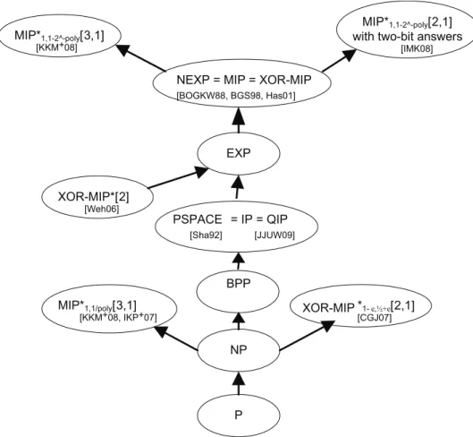
We summarize the complexity classes discussed so far in figure 3.2. This chapter concludes the motivation to study quantum mechanics from the perspective of complexity theory. In the next chapter, we will see that
3.4. INTERACTION WITH ENTANGLEMENT 25 EXP NP PSPACE [Sha92] = IP = QIP [JJUW09] P NEXP [BOGKW88, BGS98, Has01] = MIP = XOR-MIP BPP XOR-[Weh06] MIP*[2] MIP* [KKM+08, IKP+07] 1,1/poly[3,1] MIP* [KKM+08] 1,1-2^-poly[3,1] MIP*1,1-2^-poly[2,1]
with two-bit answers
[IMK08]
XOR-MIP *
[CGJ07]
1- e,½+e[2,1]
Figure 3.2: Updated Hierarchy of Complexity Classes.
the terminology of games is well adapted for the study of interactive classes with quantum mechanical concepts.
Chapter 4
Two-prover One-round Games
A better understanding of the effect of entanglement would give insight for the power of interactive classes extended with quantum mechanics. A natural framework to study these effects of nonlocality within interaction is through cooperative games with imperfect information. A cooperative game is a game in which players gain if they collaborate. The games studied have imperfect information, that is the players do not know the actions of the other players perfectly. In other words, no prover has access to the question that the other prover has received and therefore has to infer his likely actions. A game with perfect information is not interesting from the standpoint of information theory since the best actions are known in advance through the minimax decision rule [RN03]. In this thesis, we will concentrate on games with one round because of their simplicity. Note that in the game-theoretic framework, the verifier is in some cases referred to as the referee and the provers as the players.
In this chapter, we describe the framework of two-prover one-round games and explain its links with complexity theory, particularly with multi-prover interactive classes. This will serve as a basis to study the effect of quantum mechanics on these complexity classes. Following the work of [CHTW04], we prove the upper bound on the probability of winning in games for quantum provers in certain conditions. We then conclude the chapter with the description of a game that will serve as an example case in the forthcoming chapters.
28 CHAPTER 4. TWO-PROVER ONE-ROUND GAMES
4.1
Games Parameters
A two-prover one-round game is a game played by a verifier V against two provers P1 and P2 who cooperate with each other. The following definition
describes a two-prover one-round game.
Definition 4.1.1 (Two-Prover One-Round Game). A two-prover one-round game G = (X, Y, A, B, R, πXY) is defined by
• Finite sets of questions X and Y , • Finite sets of answers A and B,
• Winning Condition R : X × Y × A × B → {0, 1} and • Probability distribution πXY on the question set X × Y ,
4.2
Strategies of the Provers
For a two-prover one-round game G = (X, Y, A, B, R, πXY), the provers
share a joint strategy before interaction begins. Once the verifier is ensured that the provers cannot communicate (e.g: by physical separation), interac-tion can occur. The verifier samples quesinterac-tions (x, y) from X× Y according to the probability distribution πXY. He then sends the questions x and y
to provers P1 and P2, who respond with a ∈ A and b ∈ B, respectively.
The provers win the game against the verifier if R(x, y, a, b) = 1, otherwise, the verifier wins against the provers; R(x, y, a, b) is either 0 or 1. As a convention, the winning condition R(x, y, a, b) is rewritten R(a, b | x, y) to emphasize the fact that the answer (a, b) depends on the question (x, y). The provers can agree on a joint strategy for the game.
Definition 4.2.1 (Strategy). A strategy for the provers consists in a set S of probability distributions S(x,y) over A× B indexed by (x, y) ∈ X × Y
S = {S(x,y)}(x,y)∈X×Y. (4.1)
These can be interpreted as the provers giving joint answers (a, b) ∈ A× B to the questions (x, y) ∈ X × Y with probability S(a, b | x, y). Given that P1 has no access to question y and P2 has not access to question x, not
all probability distributions S(x,y) will be possible; we shall come back on
this issue later. The probabilities are normalized so that for all questions (x, y):
4.2. STRATEGIES OF THE PROVERS 29
∑
(a,b)
S(a, b| x, y) = 1.
We now introduce three classes of strategies based on the type of cor-related resources that the provers possess. Although, the provers are given unlimited computational power, they nonetheless cannot communicate in the interactive part of the process. However, the initial resources they share give them a certain amount of possible correlation during interaction.
In the weakest class of strategies, the class of classical or unentangled strategies, the provers are allowed to share any classical random variables before the game starts as well as any private source of randomness they wish to use once the game has started. Formally, a classical strategy for the provers P1 and P2 is described for any question pair (x, y) and answer pair
(a, b) by the following distributions S(a, b| x, y) =∑
e
p(e)S(a | x, e)S(b | y, e). (4.2)
where e can be seen as shared randomness. The optimal classical strategy is in fact deterministic since a probabilistic strategy is just a probability distribution over a finite set of deterministic strategies. So the provers can analyse every possible outcome of randomness and fix it so that it maximizes the winning probabilities of the game. We thus can see the set of classical strategies of P1 and P2 as a set of deterministic functions a(x) and b(y).
A stronger strategy class, the class of quantum strategies, encompasses strategies for which the provers are allowed to share a bipartite state |ψ⟩ ∈ CΣ×Γ. The quantum strategies of each prover consist in
perform-ing a quantum measurement for each question over their share of the state and by answering by the outcome of the measurement. Using the POVM formalism, for each x∈ X prover P1 has a POVM defined by
{Ea
x : a∈ A} ⊆ CΣ×Σ
and for each y ∈ Y prover P2 has a POVM defined by
{Eb
y : b∈ B} ⊆ CΓ×Γ
where each POVM satisfies completeness relation (2.5). Upon receiving the questions (x, y)∈ X × Y , the provers apply their POVM with respect to their question on their part of the state |ψ⟩. The outcomes (a, b) ∈
30 CHAPTER 4. TWO-PROVER ONE-ROUND GAMES
A× B of the measurements is sent to the verifier. From equation (2.6), the probability that the provers answers (a, b) ∈ A ⊗ B is given by
S(a, b| x, y) = ⟨ψ|Exa⊗ Eyb|ψ⟩. (4.3) Finally, the class of no-signalling strategies, or behavior, includes any possible strategies that cannot be used by the provers to communicate. For example, each prover could have a magical black box that can give them a kind of correlation that cannot be implemented in the physical world, provided it cannot be used to communicate. More formally, a no-signalling strategy imposes on the prover P1 that for any questions x ∈ X, y, y′ ∈ Y
and answers a ∈ A, the marginal distributions ∑
b∈B
S(a, b| x, y) = ∑
b∈B
S(a, b | x, y′).
Similarly for the prover P2, for any question y ∈ Y , x, x′ ∈ X and answers
b ∈ B, the marginal distributions ∑
a∈A
S(a, b| x, y) = ∑
b∈B
S(a, b | x′, y).
The class of strategies available to the provers directly influences the winning probability of two-prover one-round games.
Definition 4.2.2 (Winning Probability of a Strategy). In a two-prover one-round game G = (X, Y, A, B, R, πXY), the winning probability ˜ω(SK)of a
strategy S = {S(x,y)}(x,y)∈X×Y is given by
˜ ω(S) = ∑ (x,y)∈X×Y πXY(x, y) ∑ (a,b)∈A×B R(a, b| x, y)S(a, b | x, y) .
Sometimes we will say that a game is a classical game, quantum game or no-signalling game to indicate the kind of strategy used by the provers.
4.3
Value of a Game
From the winning probability ˜ω(S) of a strategy S, the value ωK(G) of a
4.3. VALUE OF A GAME 31
Definition 4.3.1 (Value of a Two-prover One-round Game). The value of a two-prover one-round game G = (X, Y, A, B, R, πXY) with strategy class
K over strategy S is given by
ωK(G) = sup S∈K ∑ (x,y)∈X×Y πXY(x, y) ∑ (a,b)∈A×B R(a, b| x, y)S(a, b | x, y) .
In particular, the value of a two-prover one-round game G with classi-cal strategy is described by ωc(G), with quantum strategies by ωq(G) and
with no-signalling strategies by ωns(G). The trivial relationship among the
different classes of strategies is
0≤ ωc(G)≤ ωq(G)≤ ωns(G)≤ 1. (4.4)
We open a parenthesis here to look at the definition of the value ωK(G) of
a game G with respect to the class of strategies K. We find a solution for the value by solving a linear program in variables S(a, b | x, y). The definition of the value constitutes the objective function. The constraints of the problem include positivity, normalization as well as the constraint imposed directly from the strategy class C. Positivity imposes that S(a, b | x, y) ≥ 1 and normalization that for all pairs (x, y):∑(a,b)S(a, b | x, y) = 1. The last constraint comes directly from the definition of the class of strategy C.
As we said, the value of a game constitutes a linear programming prob-lem referred to the primal probprob-lem. The probprob-lem of maximization in the primal problem with n variables and m constraints can be cast as a min-imization problem. This is referred as the dual problem. In optmin-imization theory, duality is the principle according to which the problem can be seen by either of the two perspectives: the primal or the dual problem. The dual problem is a linear combination of the m values in the primal problem that limit the constraints. In the dual problem, there are n dual constraints that make a lower bound on a linear combination of m dual variables. This means that even if we cannot solve the linear program, we can obtain an upper bound on the value of a game by constructing a solution to the dual program. Appendix A describes the formalism of mathematical optimiza-tion in more details.
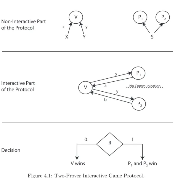
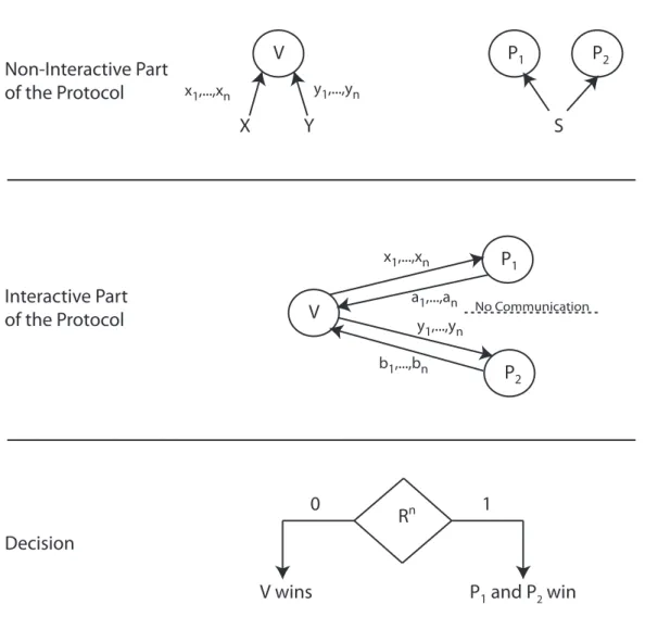
We summarize the process of interactive games in figure (4.1). The three steps of the protocol are depicted: the non-interactive part, the interaction and the decision of the verifier.
32 CHAPTER 4. TWO-PROVER ONE-ROUND GAMES Non-Interactive Part of the Protocol Interactive Part of the Protocol V P1 P2 X Y S x y V P1 P2 x y a b No Communication Decision R 0 1
V wins P1 and P2 win
Figure 4.1: Two-Prover Interactive Game Protocol.
4.4
Relationship with Complexity Theory
Besides the classification of games with respect to strategies, games are also categorized by other parameters. Two of these characterizations are: binary games and XOR games. Binary games are games for which the answers of both provers are single bits (i.e.:A = B = {0, 1}). XOR games are binary games for which the function R is a function of a⊕ b and not of a and b independently.
The relation with interactive complexity classes MIP[2, 1], ⊕MIP[2, 1], MIP∗[2, 1] and ⊕MIP∗[2, 1] should now seem evident. Consider a promise problem A = (Ayes, Ano) as introduced in definition (3.1.1). Given any
string s and a game G, if s ∈ Ayes, the value ωK(G) with respect to strategy
4.5. UPPER BOUND FOR XOR GAMES 33
Non-signalling strategies are useful since they can sometimes give an upper bound for quantum strategies in the case this bound is not known. However, for the game to be a valid proof system, the soundness must not to be 1. Otherwise, the provers will be able to cheat the verifier every time. An upper bound on the value of a game will give insight on conditions for the associated complexity class.
Promise problems represent more generally the formalism of games com-pared to languages since it is possible that some inputs will never occur and therefore there is no need for the corresponding output to be defined. Lan-guages have to be decision problems over all possible inputs.
Next, we prove an interesting result that puts an upper bound on the value of a XOR game with quantum strategies as a function of the classical value for that game. This upper bound will serve to prove the quantum value of the game in section 4.6.
4.5
Upper Bound for XOR Games
In [CHTW04], upper bounds for the value any XOR game with quantum strategies are proven. Preliminary to those results, it is demonstrated that the optimal value of two-prover binary games with quantum strategies is obtained by the provers doing projective measurements on their part of the shared state. Moreover, the parts of the shared state are of equal di-mension. Therefore, in the search of an optimal strategy, only projective measurements have to be considered.
We describe the orthogonal projections M0 and M1 of prover P1 subject
to M0 + M1 = I in terms of the observable M = M0− M1 and similarly with N = N0 − N1 for prover P
2. The observables of the two-outcome
projective measurement form a Hermitian matrix with eigenvalues +1 and −1 that can be mapped to answers 0 and 1 in that order.
A necessary result has to be stated before proving the bounds. The result in [Tsi87] relates the problem of finding the probability ⟨ψ|Ma
x⊗Nyb|ψ⟩ that
the provers answer by (a, b) ∈ A ⊗ B to questions (x, y) ∈ X ⊗ Y to the classical problem of finding two real unit vectors.
Theorem 4.5.1 ([Tsi87]). Let X and Y be finite sets and let |ψ⟩ be a pure quantum state with support on a bipartite Hilbert space H = A ⊗ B such that dim(A ) = dim(B) = n. For each x ∈ X and y ∈ Y , let Mx and Ny be