HAL Id: hal-02022629
https://hal.archives-ouvertes.fr/hal-02022629
Submitted on 17 Mar 2019
HAL is a multi-disciplinary open access
archive for the deposit and dissemination of
sci-entific research documents, whether they are
pub-lished or not. The documents may come from
teaching and research institutions in France or
abroad, or from public or private research centers.
L’archive ouverte pluridisciplinaire HAL, est
destinée au dépôt et à la diffusion de documents
scientifiques de niveau recherche, publiés ou non,
émanant des établissements d’enseignement et de
recherche français ou étrangers, des laboratoires
publics ou privés.
Efficient Bark Recognition in the Wild
Rémi Ratajczak, Sarah Bertrand, Carlos Crispim-Junior, Laure Tougne
To cite this version:
Rémi Ratajczak, Sarah Bertrand, Carlos Crispim-Junior, Laure Tougne. Efficient Bark Recognition
in the Wild. International Conference on Computer Vision Theory and Applications (VISAPP 2019),
Feb 2019, Prague, Czech Republic. �10.5220/0007361902400248�. �hal-02022629�
Efficient Bark Recognition in the Wild
R´emi Ratajczak
1,2,3, Sarah Bertrand
1, Carlos Crispim-Junior
1and Laure Tougne
11Univ Lyon, Lyon 2, LIRIS, F-69676 Lyon, France 2Unit´e Cancer et Environnement, Centre L´eon B´erard, Lyon, France 3Agence de l’Environnement et de la Maˆıtrise de l’Energie, Angers, France {remi.ratajczak, sarah.bertrand, carlos.crispim-junior, laure.tougne}@liris.cnrs.fr
Keywords: Bark recognition, texture classification, color quantification, dimensionality reduction, data fusion.
Abstract: In this study, we propose to address the difficult task of bark recognition in the wild using computationally efficient and compact feature vectors. We introduce two novel generic methods to significantly reduce the dimensions of existing texture and color histograms with few losses in accuracy. Specifically, we propose a straightforward yet efficient way to compute Late Statistics from texture histograms and an approach to iteratively quantify the color space based on domain priors. We further combine the reduced histograms in a late fusion manner to benefit from both texture and color cues. Results outperform state-of-the-art methods by a large margin on four public datasets respectively composed of 6 bark classes (BarkTex, NewBarkTex), 11 bark classes (AFF) and 12 bark classes (Trunk12). In addition to these experiments, we propose a baseline study on Bark-101, a new challenging dataset including manually segmented images of 101 bark classes that we release publicly.
1
INTRODUCTION
Automatic bark recognition applied to tree species classification is an important problematic that has gained interest in the computer vision community. It is an interesting challenge to evaluate texture classi-fication algorithms on color images acquired in the wild. Due to their low inter-class variability and high intra-class variability, bark images are indeed consid-ered as difficult to classify for a machine as for a hu-man.
In the context of tree species classification, barks have interesting properties compared to other
com-monly used attributes (e.g. leaves, fruits, flowers,
etc.). Firstly, they are non-seasonal: Whatever the season, the texture of a bark will not change. This property is particularly important to classify a tree during winter, when no leaves or fruits are present. Secondly, bark textures rarely change through short time periods (i.e. a year basis), but they do change over long periods (i.e. tenth year basis). This property enables the use of age priors for bark classification, but it makes the recognition even more challenging when these priors are unavailable. Finally, barks are easier to isolate and to photograph compared to fruits and leaves that may be unreachable on tall trees. In result, bark images have been used to recognize tree
species either alone [Bertrand et al., 2017], or in com-bination with other tree’s attributes [Bertrand et al., 2018]. In order to recognize trees, mobile
applica-tions like Folia1 [Cerutti et al., 2013] have been
de-veloped. These applications assume that users do not necessarily have an Internet connection, which is a very common situation in the wild. They should work on embedded devices by seeking a trade-off between accuracy, time complexity and space complexity to ensure state-of-the-art recognition rates while avoid-ing unnecessary energy consumption. Consequently, most of these applications are based on efficient hand-crafted filters.
In this context, we propose two novel approaches to drastically reduce the dimensionality of both tex-ture and color featex-ture vectors, while preserving ac-curacy. We focused our work on handcrafted meth-ods and decided not to use end-to-end Deep Convo-lutional Neural Networks (DCNNs) because existing datasets are not well suited to both train and evaluate deep learning algorithms: They contain relatively few images, up to 1632 for 6 classes in [Porebski et al., 2014]. Moreover, DCNNs have both high time and space complexity that make them unsuitable for em-bedded usage.
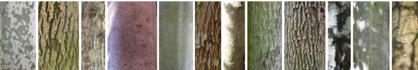
Figure 1: Examples of bark images from Bark-101 dataset.
To overcome the few numbers of segmented bark classes in existing datasets; up to 12 in [ ˇSvab, 2014]; we also release a novel and even more challenging dataset made of 101 segmented bark classes in high
resolution: Bark-1012(see Section 2.1). This dataset
has been conceived with a clear focus on the number of classes, involving high intra-class and low inter-class variabilities (see Figure 1).
The remainder of this study is organized as fol-low. Section 2 presents previous work related to bark recognition in the wild. Section 3 introduces and de-tails the proposed algorithms for efficient dimension-ality reduction of texture and color histograms. Sec-tion 4 presents the experiments we carried out and dis-cusses the results.
2
RELATED WORK
This section presents existing bark datasets and state-of-the-art methods for bark recognition.
2.1
Datasets
We propose to describe four state-of-the-art datasets that are publicly available and commonly used in the literature. In complement, we release an even more challenging dataset: Bark-101. The characteristics of these datasets are detailed below and summarized on Table 1.
BarkTex and NewBarkTex. BarkTex was the first dataset specialized on bark recognition. It was introduced by R. Lakmann [Lakmann, 1998]. It is composed of 6 classes, each corresponding to a dif-ferent tree species. Each class contains 68 color im-ages of trunks for a total of 408 imim-ages. The trunks are spatially centered in the images, but some back-ground can appear depending on the width of the trunk. NewBarkTex is derived from BarkTex. It was proposed in [Porebski et al., 2014] and it is also com-posed of 6 classes. A region of interest (ROI) of size 128x128 pixels was cropped from the center of the images of BarkTex. Then the ROI was separated in 4 sub-images of 64x64 pixels. Half of the sub-images
2http://eidolon.univ-lyon2.fr/~remi1/Bark-101/
were kept for training and the second half for testing. Therefore, NewBarkTex is made of 272 images per class for a total of 1632 images.
Trunk12. It is a bark dataset created in 2014 by Matic ˇSvab [ ˇSvab, 2014]. It consists of 360 color im-ages of barks corresponding to 12 different species of tree found in Slovenia. Each class consists of about 30 images. All images were taken with the same camera in the same conditions (20 cm distance, multiple trees per class, avoiding moss, same light conditions, taken in upright position).
AFF. This bark dataset was presented in [Wendel et al., 2011]. It has 11 classes of bark from the most common Austrian trees. It is composed of 1082 color images of bark. In AFF, tree species are separated in sub-classes according to the age of the tree. The texture of the trunk changes during the lifetime of a tree, starting from a smooth to a more and more coarse texture. In this study, we have chosen to not separate the classes according to the age of the trees.
Bark-101. We built the Bark-101 dataset among
the PlantCLEF3identification task, part of the
Image-CLEF challenge, designed to compare plant recogni-tion algorithms. PlantCLEF contains photos of mul-tiple yet not segmented plant organs (leaf, flower, branch, steam, etc.) taken by people in various un-supervised shooting conditions and gathered through
the mobile application Pl@ntNet4. More than 500
herb, tree and fern species centered on France are present in PlantCLEF [Go¨eau et al., 2014]. To con-struct Bark-101, we kept the tree stems available from PlantCLEF (i.e. the barks), and have manually seg-mented them to remove undesirable background in-formation. We decided to follow the authors of [Wen-del et al., 2011] by not constraining the size of the seg-mented images in Bark-101. This choice was made to simulate real world conditions assuming a perfect stem segmentation. As a matter of fact, in a real world setting not all trees would have the same di-ameter and not all users would photograph them at a pre-defined distance. The Bark-101 dataset is there-fore composed of 101 classes of tree barks from var-ious age and size for a total of 2592 images. Images
3https://www.imageclef.org/lifeclef/2017/plant 4https://identify.plantnet-project.org/
Table 1: Characteristics of bark datasets.
Dataset information BarkTex NewBarkTex Trunk12 AFF Bark-101
Classes 6 6 12 11 101
Total images 408 1632 393 1082 2592
Images per classes 68 272 30-45 16-213 2-138 Image size 256x384 64x64 1000x1334 1000x(478-1812) (69-800)x(112-804)
Illumination change 3 3 7 3 3
Scale change 3 3 7 3 3
Noise (shadows, lichen) 7 7 7 3 3
Train / Test splits 7 50/50 7 7 50/50
in Bark-101 contain noisy data like shadows, mosses or illumination changes (see Figure 1). Due to the unsupervised acquisition of the images and the varia-tion of bark textures over the lifespan of the tree, there is a high intra-class variability in Bark-101. Further-more, a large number of classes naturally leads to a small inter-class variability since the number of vi-sually similar species increases with the number of species. Consequently, Bark-101 can be considered as a challenging dataset in the context of bark recog-nition. We further demonstrate this statement in the experiments presented in Section 4.
2.2
Existing methods
Bark recognition is often considered as a texture
classification problem. In [Wan et al., 2004] the
authors compared different statistical analysis tools for tree bark recognition, like co-occurrence ma-trices, grayscale histogram analysis and run-length method (RLM). The use of co-occurrence matrices on grayscale bark images is also present in [Huang et al., 2006b]. The authors combined them with fractal di-mensions to characterize the self-similarity of bark textures at different scales. Spectral methods, such as Gabor filters, are also used. In [Huang et al., 2006a], the authors demonstrated that only four wave orienta-tions and 6 scales are sufficient to identify tree species by their bark. To avoid losing the information pro-vided by color, Wan et al. [Wan et al., 2004] applied their grayscale method individually to each channel of the RGB space. In [Baki´c et al., 2013], different color spaces were used to characterize color informa-tion, including RGB and HSV spaces. The authors of [Bertrand et al., 2017] proposed to combine texture and color hues in a late fusion manner. First, they ex-tracted orientation features using Gabor filters. Sec-ondly, they combined these features with a sparse rep-resentation of bark contours by encoding the intersec-tions of Canny edges with a regular grid. Lastly, they described bark colors using the hue histogram from the HSV color space. The resulting descriptor proved to increase the classification rate of tree recognition when combined with leaves [Bertrand et al., 2018].
Other commonly used descriptors for bark classi-fication are Local Binary Pattern-like (LBP-like) de-scriptors that were inspired by the original LBP ter proposed by [Ojala et al., 2001]. LBP-like fil-ters are generic local texture descriptors parametrized over a (P, R) neighborhood, with P the number of
pixel neighbors and R the radii. In the case of a
multiscale filter, the number Rs of radii R is strictly
greater than 1. LBP-like filters encode textural pat-terns with binary codes, whose aggregation result in
a texture histogram of high dimension (e.g. Rs×
2P for the original LBP). Recently, the authors of
[Boudra et al., 2018] proposed a texture descriptor called Statistical Macro Binary Pattern (SMBP) in-spired by LBP. SMBP encodes the information be-tween macrostructural scales with a representation us-ing statistical characteristics for each scale. The de-scriptor increases the classification rate on two barks
datasets compared to the state of the art. In
[Al-ice Porebski, 2018], the authors demonstrated the ac-curacy of color LBP-like descriptors with different color spaces, achieving above state-of-the-art perfor-mance, but with a very high dimensional feature vec-tor. Recent works on texture classification in the wild are also of interest for bark recognition. In particu-lar, the Light Combination of Local Binary Patterns (LCoLBP), proposed by [Ratajczak et al., 2019], and the Completed Local Binary Pattern (CLBP), pro-posed by [Guo, Z. et al., 2010], obtained equivalent results to popular DCNNs on historical aerial images classification for a small computational cost. Since the CLBP filter is often used as a baseline for bark recognition based on LBP-like filters [Junmin Wang, 2017] the LCoLBP may be a suitable candidate for bark recognition in the wild.
3
PROPOSED METHODS
Bark images acquired in the wild represent objects with discriminative texture patterns and colors. To represent these characteristics considering a trade-off between accuracy and feature space complexity, we propose two novel complementary methods to effi-ciently reduce the number of texture and color
fea-𝑅1 𝑅3 𝑅5 . . . . 𝑅𝑠× 𝑁ℎ× 2|𝒑=𝟖 𝑃 2 𝐿𝐶𝑜𝐿𝐵𝑃 𝑃 = 8 𝑅 = 1,3,5 𝑅𝑠= 3 𝑁ℎ= 5 𝑅𝑠× 𝑁ℎ× 𝑁𝑠 (= 105 𝑏𝑖𝑛𝑠) 1 0 mean variance entropy max min median kurtosis 1 0 . . . 1 0 . . . . . . 𝑅1 𝑅3 𝑅5 (= 240 𝑏𝑖𝑛𝑠) 80 16 32 48 64 80 16 32 48 64 𝐿𝑆-𝐿𝐶𝑜𝐿𝐵𝑃 80 16 32 48 64 . . . .
transpose & concatenate
. . . . . . . .
𝑁𝑠= 7
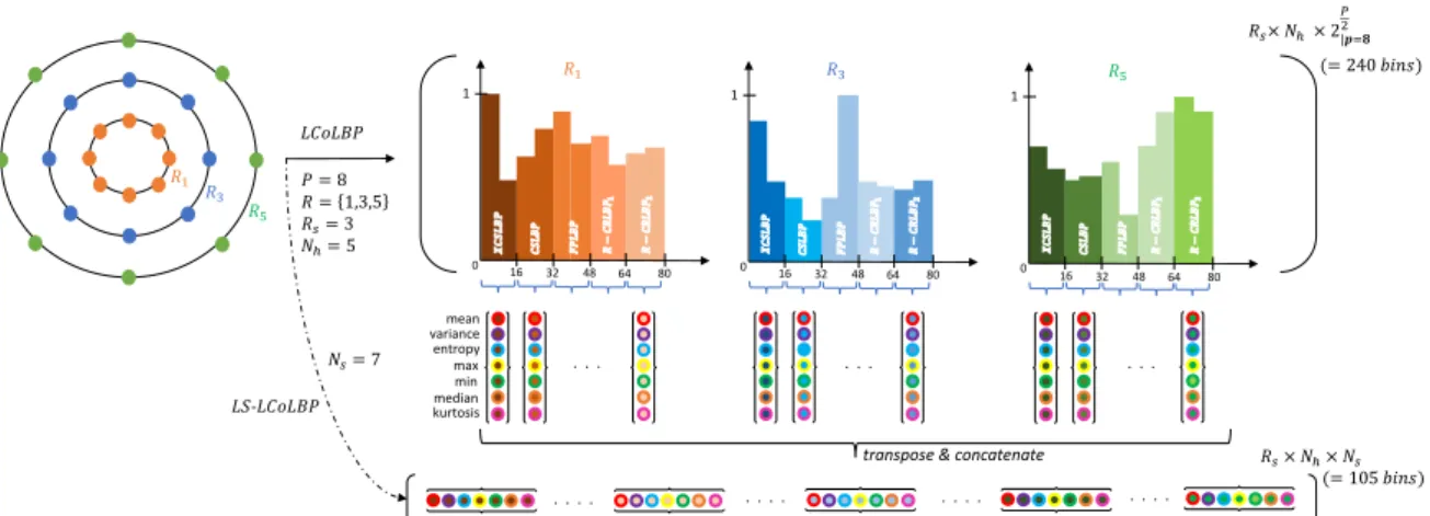
Figure 2: Late Statistics (LS) from a Light Combination of Local Binary Patterns (LCoLBP) with a 3-radii neighborhood (Rs= 3), 8 neighbors P, and 7 statistics Ns. Colored dots denote the statistics (outer colors) obtained from the Nh= 5 sub-histograms included in the LCoLBP histogram for each radius (inner colors). This configuration yields a 2.3 reduction factor.
tures. We considered these cues individually before combining them in a late fusion manner (concatena-tion). For the texture cues, we followed the com-mon use of LBP-like filters. Based on these filters, we developed a generic yet efficient statistical repre-sentation which preserves filters’ properties and does not require re-sampling or mapping operations (see Section 3.1). For the color cues, we were inspired by [Bertrand et al., 2017] and built a task-guided low dimensional histogram representation upon the HSV color space using bark priors (see Section 3.2).
3.1
From Textures to Late Statistics
We define the Late Statistics as a combination of statistical features calculated from LBP-like texture
histograms. Considering a texture histogram Ht,
it-self made of the concatenation of Nhknown and
or-dered sub-histograms {h1, h2, ..., hNh}, we calculate
Ns Late Statistics independently for each hi with i ∈
{1, ..., Nh}. Late Statistics are then concatenated in
the same order as the hi sub-histograms. Assuming
a single Ht per LBP-like radius, this process results
in a vector made of Rs× Ns× Nhfeatures, where Rs
is the number of radii (i.e. scales). It is represented
with Ns= 7 statistics and a grayscale 3-radii (Rs= 3)
LCoLBP filter on Figure 2. Note that each rotation of the R-CRLBP [Ratajczak et al., 2018], a sub-filter of the LCoLBP, is considered as an independent filter in this study.
Late statistics are defined as late in opposition to the early statistics proposed by [Boudra et al., 2018]. In [Boudra et al., 2018], the authors calculated statis-tics before calculating the texture histogram by re-sampling the local textural patterns of a LBP-like
fil-ter. In consequence, the statistical approach proposed by Boudra et al. would require new implementations with error-prone re-sampling operations to be applied to other LBP-like filters. The Late Statistics evade this constraint by considering texture histograms that have been already calculated. They do not need to operate on the local textural patterns but rather on the global histogram representations, so that they do not require any modification of the descriptor implemen-tations (i.e. no re-sampling).
Due to their nature, Late Statistics are expected to preserve common descriptor properties, like rota-tion and global illuminarota-tion invariance. This point should make the Late Statistics at least as robust to condition changes as the descriptors themselves. Fur-thermore, it should be observed that, similarly to the
earlystatistics used by [Boudra et al., 2018], the Late
Statistics naturally behave as a spatial normalization algorithm: A histogram will be summarized with a
fixed number of statistics Ns whatever its number of
bins. This property is particularly useful to combine different histograms in a balanced feature vector that contains the same quantity of information for each texture pattern.
Finally, one may observe that Late Statistics are an efficient way to summarize textural information in a very similar manner as Haralick features [Haralick et al., 1973]. However, while Haralick features repre-sent statistics calculated directly from an image, Late Statistics benefit from the efficient LBP-like represen-tation of textures.
0
b
add & shift add & shift
0
Iteration 2
N-1 to N-2 bins
add & shift
0 Iteration 1 N to N-1 bins Iteration 3 N-2 to N-3 bins Output N-3 bins I 𝑏𝑚, 𝐼 𝑏𝑚 = 𝑎𝑟𝑔𝑚𝑖𝑛(𝐼 𝑏 ) 𝑏𝑚1, 𝐼 𝑏𝑚1 = min(𝐼 𝑏𝑚− 1 , 𝐼 𝑏𝑚+ 1 ) 𝑏𝑚2, 𝐼 𝑏𝑚2 = m𝑎𝑥(𝐼 𝑏𝑚− 1 , 𝐼 𝑏𝑚+ 1 ) b I I I b b 𝑏 0
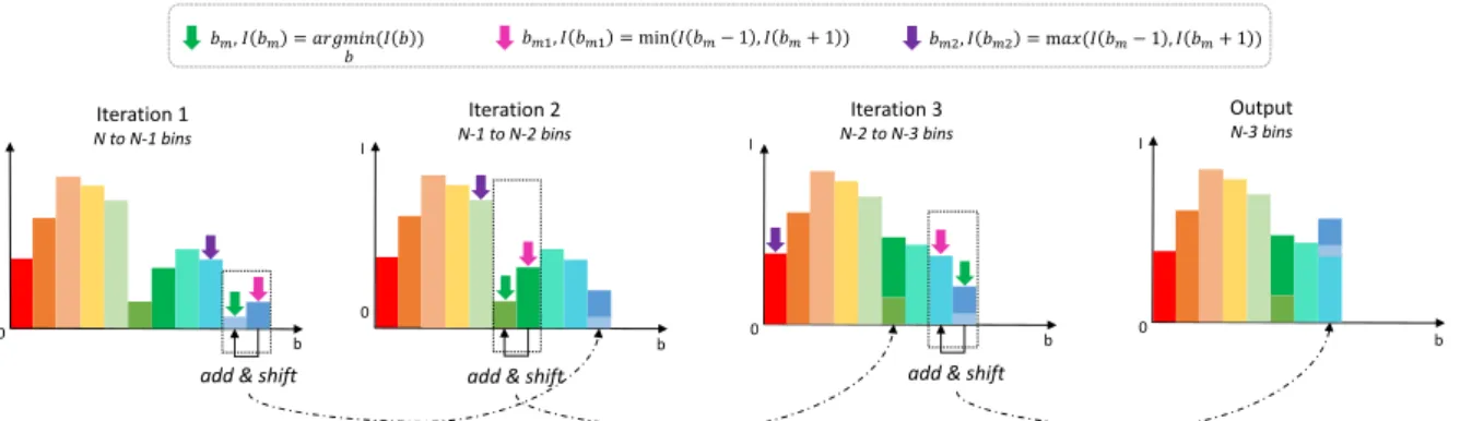
Figure 3: Schematic of the color histogram reduction applied with 3 iterations. The number of bins in the histogram is reduced by 1 after each iteration. The reduction is performed using a local add and shift strategy on the bin b with the smallest intensity I(b). A look-up table is used to map the modified bins.
3.2
Efficient Colors
We discussed in Section 2 that several bark descrip-tors work on grayscale images and that a few of them also include color data. Among these descrip-tors, hue information is commonly used [Baki´c et al., 2013, Bertrand et al., 2017]. The size of a hue his-togram H is usually of 360 bins. However, this value (360) cannot be stored on a single byte. For sam-pling reasons, it is preferable to transpose the hue color range [0;359] into the range [0;179] than into the range [0;255]. Therefore, the size of the hue his-togram is 180 bins, which represents a feature vector of a quite high dimensionality for task-specific appli-cations with color priors, like bark recognition in the wild. As visible on Figure 1, barks have dominant variations of brown, green and yellow colors. Based on this observation, we may expect that other colors like blue or purple may not provide significant contri-bution to the hue signature of a bark. However, com-pletely removing these colors may result in less dis-criminant histograms, making the bark classification process even more difficult.
To reduce the size of the hue histogram, we pro-pose to merge the least represented colors through a non-destructive iterative process. For a given dataset
Dmade of k color images splitted into a train set Tr
and a test set Te, we first calculate and sum all the hue
histograms of the images in Tr. We obtain a summed
hue histogram Hs from the train set Tr ⊂ D. This
summed histogram Hs is supposed to represent the
color prior on the whole dataset D. Secondly, on the
summedhistogram Hs, we iteratively add the
popula-tion of the bin b having the smallest intensity value (i.e. the smallest population) to the population of its neighbor of minimal population. After adding these bins, we shift the histogram to the left in order to re-duce its dimension. The iteration process is stopped
when the desired size, fixed by the user, is reached (see Section 4). Attention should be brought to the circularity of the hue channel in the HSV color space. The order and position of the add and shift operations
are stored in a look-up table M. On the test set Te,
the look-up table M is then used to calculate the
re-duced histograms of the input images LTeby applying
the add and shift operations in the same order as in
Tr. Consequently, the reduced histogram for an image
lTe ∈ LTe is generated in regard to the summed
his-togram, thus taking into account the color prior of the data. The add and shift process is illustrated on Fig-ure 3.
4
EXPERIMENTS AND RESULTS
4.1
Experimental Setup
For our experiments, we considered two state-of-the-art LBP-like filters made of complementary sub-descriptors to assess the efficiency of the Late Statis-tics: The Light Combination of Local Binary Patterns (LCoLBP) and the Completed Local Binary Pattern (CLBP). As explained in Section 2, these descrip-tors are efficient texture filters which obtained DC-NNs like accuracy rates on texture in the wild datasets [Ratajczak et al., 2019]. Since these filters may re-sult in very high dimensional histograms, we consid-ered a constant number of neighbors P on a 3-radii
(Rs= 3) neighborhood: (P = 8, R = {1, 3, 5}). To
as-sess the effectiveness of the Late Statistics on both mapped and unmapped LBP-like representations, we followed [Ratajczak et al., 2019] and applied the LCoLBP without any mapping, resulting in a
his-togram of Rs× 5 × 24bins (Nh= 5) with a (P = 8, R =
{1, 3, 5}) neighborhood. On the other hand, we
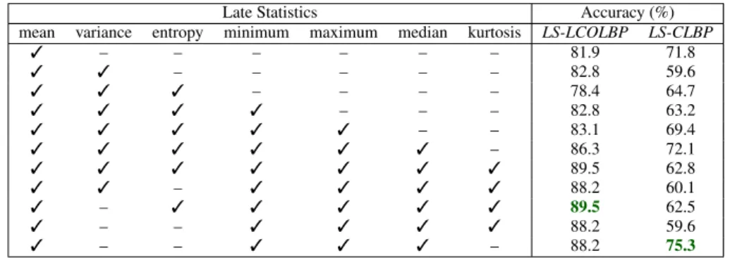
in-Table 2: Ablation study for the Late Statistics of the LCoLBP and CLBP filters on the BarkTex dataset. Late Statistics Accuracy (%)
mean variance entropy minimum maximum median kurtosis LS-LCOLBP LS-CLBP
3 – – – – – – 81.9 71.8 3 3 – – – – – 82.8 59.6 3 3 3 – – – – 78.4 64.7 3 3 3 3 – – – 82.8 63.2 3 3 3 3 3 – – 83.1 69.4 3 3 3 3 3 3 – 86.3 72.1 3 3 3 3 3 3 3 89.5 62.8 3 3 – 3 3 3 3 88.2 60.1 3 – 3 3 3 3 3 89.5 62.5 3 – – 3 3 3 3 88.2 59.6 3 – – 3 3 3 – 88.2 75.3
troduced by [Ojala et al., 2001] with the CLBP filter, resulting in a histogram of 3 × (2 + 2 × 10) bins in-stead of 3 × (2 + 2 × 256) bins without mapping for the same neighborhood.
We considered commonly used statistics in our ex-periments: Mean, variance, entropy, minimum, max-imum, median and kurtosis. Among them, we car-ried out an ablation study through gridsearch to de-termine the best combination of Late Statistics for each texture filter as presented on Table 2 for Bark-Tex. Ablation results obtained on other datasets were in concordance with Table 2 as well as with the fol-lowing observations. On Table 2, we can observe that naively adding more Late Statistics (first seven lines) may decrease the accuracy of the texture repre-sentations. We also demonstrate that the Late Statis-tics should be carefully and individually selected for each texture filter in order to maximize the accuracy rate (up to a difference of ˜15% on Table 2). This phenomenon highlight a minor drawback of the Late Statistics: While they are effective and easy to im-plement, they increase the number of parameters to
tune. Therefore, the number of statistics Ns was set
to 6 for the LCoLBP and 4 to CLBP. We did not ap-ply the Late Statistics on the first sub-histogram of the CLBP filter because it is made of only two bins. Late Statistics of the LCoLBP filter (LS − LCoLBP) result
in Rs× 5 × Ns features. Late Statistics of the CLBP
filter (LS −CLBP) result in Rs× (2 + 2 × Ns) features.
Concerning the bark colors, we verified that bark images are actually made of dominant colors on the extensive train set of the Bark-101 dataset because of the large variability of bark images and classes avail-able (see Section 2.1). The summed hue histogram
Hs for this dataset is visible on Figure 4. Based on
this figure, we can observe that the majority of barks present brownish, yellowish and greenish hues. In order to define a suitable dimension for the reduced color histogram, we observed the evolution of the classification rate according to the strategy defined in Section 4.2 on Bark-101 dataset (Figure 5). Despite
small variations in the species classification rate when quantifying the histogram, we can see that the accu-racy remains approximately constant over 30 bins. As the other bark datasets present smaller variance and are thus less representative of real world conditions, we decided to set the size of the reduced hue his-togram to 30 bins regardless of the bark dataset. We remind that a look-up table, to obtain the reduced his-tograms, is calculated for each dataset independently: Only the size of 30 bins has been fixed using Bark-101.
4.2
Evaluation and Metrics
We separated our evaluation into two classification
strategies, c1and c2, depending on the dataset
orga-nizations, visible on Table 1, and previous
state-of-the-art experiments. Strategy c1 stands for the
clas-sical train/test strategy. In c1, a part of the dataset is
used for training and the rest of the dataset is used for
testing. We performed c1on NewBarkTex and
Bark-101 following the train and test splits (50%/50%)
pro-vided by the authors. Strategy c2 is the
leave-one-out strategy (LOO). In c2, we considered an ensemble
S of N samples and we performed N iterations. At
each iteration i ∈ {1, ..., N}, we used a different sam-ple s(i) of S for evaluation (i.e. testing) and all the other samples of S − {s(i)} for training. If the eval-uation sample s(i) was successfully classified, the
re-Figure 4: Summed histogram of the hue channels from the train set of the Bark-101 dataset.
sult of the corresponding iteration was set to 1, and to 0 otherwise. The final accuracy was obtained by averaging the results of all iterations. In accordance
with [Boudra et al., 2018], we performed c2on
Bark-Tex, Trunk12 and AFF. For both c1 and c2 we used
the top-1 accuracy and a K-Nearest Neighbor clas-sifier (KNN) with K = 1 and the L1 distance. The 1-NN is the most commonly used classifier in the context of bark and texture recognition. The L1 dis-tance has been chosen arbitrarily. Additionally, for
c1, and in accordance with [Alice Porebski, 2018], we
used a multi-class non-linear Support Vector Machine (SVM) with radial basis kernel. The parameters of the SVM classifier have been optimized by grid search for each dataset and for each feature vector.
4.3
Results and Discussion
Results are visible on Table 3 and Table 4. They have been obtained considering the evaluation strategies described in Section 4.2. Highest accuracy rates from other studies have been reported and marked with a right-top star symbol. Specifically, for AFF, Trunk12 and BarkTex, we reported the results obtained with
MSLBP*and SLBP* from [Boudra et al., 2018]. The
results for NewBarkTex were reported for Wang17* [Junmin Wang, 2017], Sandid16* [Sandid and Douik, 2016], and Porebski18* [Alice Porebski, 2018]. We also considered the results proposed by the methods of [Bertrand et al., 2017] that we renamed GWs and GWs/H180. All other results correspond to our own implementations using OpenCV 3.4 in C++ for the texture and color descriptors. Scikit-learn in Python has been used for the Late Statistics and the classi-fiers. The texture cues were calculated on grayscale images. The color cues were calculated on bark im-ages in HSV color space. The following sections dis-cuss the results obtained.
Figure 5: Accuracy of the reduced hue histogram on the Bark-101 dataset depending on the final number of bins.
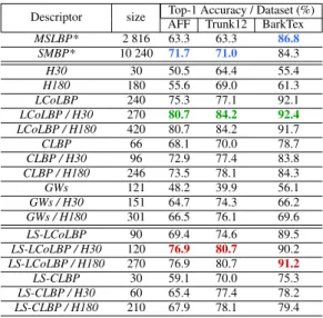
Table 3: Results of Late Statistics and reduced color his-tograms with KNN and leave-one-out strategy. Blue: High-est results of the literature. Green: highHigh-est results overall. Red: Highest late statistics results.
Top-1 Accuracy / Dataset (%) Descriptor size
AFF Trunk12 BarkTex MSLBP* 2 816 63.3 63.3 86.8 SMBP* 10 240 71.7 71.0 84.3 H30 30 50.5 64.4 55.4 H180 180 55.6 69.0 61.3 LCoLBP 240 75.3 77.1 92.1 LCoLBP / H30 270 80.7 84.2 92.4 LCoLBP / H180 420 80.7 84.2 91.7 CLBP 66 68.1 70.0 78.7 CLBP / H30 96 72.9 77.4 83.8 CLBP / H180 246 73.5 78.1 84.3 GWs 121 48.2 39.9 56.1 GWs / H30 151 64.7 74.3 66.2 GWs / H180 301 66.5 76.1 69.6 LS-LCoLBP 90 69.4 74.6 89.5 LS-LCoLBP / H30 120 76.9 80.7 90.2 LS-LCoLBP / H180 270 76.9 80.7 91.2 LS-CLBP 30 59.1 70.0 75.3 LS-CLBP / H30 60 65.4 77.4 78.2 LS-CLBP / H180 210 67.9 78.1 79.4
Table 4: Results achieved on NewBarkTex and Bark-101. Top-1 Accuracy / Dataset(%) NewBarkTex Bark-101 Descriptor size KNN SVM KNN SVM Porebski18* 10 752 – 92.6 – – Wang17* 267 84.3 – – – Sandid16* 3 072 – 82.1 – – H30 30 48.0 50.6 19.1 20.4 H180 180 48.5 53.6 22.2 20.9 LCoLBP 240 78.8 89.3 34.2 41.9 LS-LCoLBP 90 66.5 79.4 28.3 30.1 LS-LCoLBP / H30 120 71.9 82.0 27.6 32.1 LS-LCoLBP / H180 270 72.3 82.2 27.8 31.0 GWs / H30 151 60.4 74.1 28.2 31.7 GWs / H180 301 54.1 63.6 31.8 32.2 4.3.1 Color cues
On Tables 3 and 4, we can observe that all the tex-ture filters obtained higher accuracy rates when com-bined with color histograms of both 30 bins (H30) and 180 bins (H180). As a reminder, H30 is the reduced hue histogram and H180 is the complete hue his-togram. When used alone, H180 is, in average, only 3.3% more accurate than H30 on AFF, Trunk12 and BarkTex. However, we found that when combined with grayscale textures, the contribution of both color representations is equivalent. These results demon-strate the efficiency of the color histogram reduc-tion algorithm presented in Secreduc-tion 3.2. Moreover, these results confirm that color cues seem to be non-negligible features for bark recognition, in opposition to the assumption made by [Boudra et al., 2018] but in accordance with [Junmin Wang, 2017].
4.3.2 Late statistics
The Late Statistics decreased the size of the evaluated texture features with a multiplicative factor between 2.7 for the LCoLBP and 2.2 for the CLBP with an averaged reduction in accuracy of only 5.5% overall. The Late Statistics seem particularly efficient with a leave-one-out strategy (Table 3) with an averaged dif-ference of 3.7% between the LCoLBP and the LS-LCoLBP, and an averaged difference of 4.1% between the CLBP and the LS-CLBP. On the other hand, they are slightly less effective on the Train/Test strategies. These results may be explained by a lack of training data resulting in an under accurate statistical descrip-tion of the per-class texture histograms.
4.3.3 Overall performances
We can observe that the Late Statistics combined with the reduced hue histograms H30 outperform prior works on the AFF, Trunk12 and BarkTex datasets. LS-LCoLBP/H30 is in averaged 6.3% more accurate than the methods compared in [Boudra et al., 2018]. Moreover, it is about 100 times smaller than SMBP*. On NewBarkTex, Late Statistics combined with hue histograms and a SVM classifier achieve similar re-sults to Sandid16* with an accuracy of 82.0%. We observe that our method (LS − LCoLBP/H30) ob-tained slightly lower results than the most accurate algorithms from the literature on this dataset, but it does have a significantly smaller feature vector which is about 30 times smaller than Sandid16* and 100 times smaller than Porebski18*. On Bark-101, we can observe the lowest accuracy rates for all compared methods over all the datasets. These results are ex-plained by the higher number of classes in Bark-101 compared to existing datasets. It also demonstrates the challenge proposed by Bark-101. However, most methods including GWs/H30 achieved a top-1 recog-nition rate about 30%, which is far above the random guess of 0.9%.
5
CONCLUSION
In this study, we compared recent state-of-the-art descriptors in the context of tree bark recognition in the wild. We proposed two novel algorithms to re-duce the dimensionality of texture and color features vectors. We showed that the proposed algorithms out-perform state-of-the-art methods on four bark datasets with a considerable gain in space complexity. We be-lieve that these methods can be generalized on other histogram-like feature vectors. Furthermore, we re-leased a new dataset made of 101 bark classes of
seg-mented images with high intra-class variability. We demonstrated that the proposed dataset is particularly challenging for existing methods, enforcing the need for future prospects on bark recognition. Future work will investigate the proposed methods as a lightweight representation with multiple color spaces. We will also evaluate the proposed algorithms on mobile plat-forms, such as smartphones, to assess their perfor-mances on real-world settings.
ACKNOWLEDGEMENT
This work is part of ReVeRIES project (Recon-naissance de V´eg´etaux R´ecr´eative, Int´eractive et Ed-ucative sur Smartphone) supported by the French Na-tional Agency for Research with the reference ANR-15-CE38-004-01, and part of the French Environment and Energy Management Agency, Grant TEZ17-42.
REFERENCES
Alice Porebski, Vinh Truong Hoang, N. V. D. H. (2018). Multi-color space local binary pattern-based feature selection for texture classification. Journal of Elec-tronic Imaging, 27:27 – 27 – 15.
Baki´c, V., Mouine, S., Ouertani-Litayem, S., Verroust-Blondet, A., Yahiaoui, I., Go¨eau, H., and Joly, A. (2013). Inria’s participation at imageclef 2013 plant identification task. In CLEF Working Notes.
Bertrand, S., Ameur, R. B., Cerutti, G., Coquin, D., Valet, L., and Tougne, L. (2018). Bark and leaf fusion sys-tems to improve automatic tree species recognition. Ecological Informatics.
Bertrand, S., Cerutti, G., and Tougne, L. (2017). Bark recognition to improve leaf-based classification in di-dactic tree species identification. In VISAPP. Boudra, S., Yahiaoui, I., and Behloul, A. (2018). Plant
iden-tification from bark: A texture description based on statistical macro binary pattern. In ICPR.
Cerutti, G., Tougne, L., Mille, J., Vacavant, A., and Coquin, D. (2013). Understanding leaves in natural images - a model-based approach for tree species identification. Computer Vision and Image Understanding.
Go¨eau, H., Joly, A., Bonnet, P., Selmi, S., Molino, J.-F., Barth´el´emy, D., and Boujemaa, N. (2014). Lifeclef plant identification task 2014. In CLEF2014 Work-ing Notes. WorkWork-ing Notes for CLEF 2014 Conference, Sheffield, UK, September 15-18, 2014, pages 598– 615. CEUR-WS.
Guo, Z., Zhang, L., and Zhang, D. (2010). A Completed Modeling of Local Binary Pattern Operator for Tex-ture Classification. IEEE TIP, 19(6).
Haralick, R. M., Shanmugam, K., and Dinstein, I. (1973). Textural Features for Image Classification. IEEE Transactions on Systems, Man, and Cybernetics.
Huang, Z.-K., Huang, D.-S., Du, J.-X., Quan, Z.-H., and Guo, S.-B. (2006a). Bark classification based on gabor filter features using rbpnn neural network. In Interna-tional conference on neural information processing, pages 80–87. Springer.
Huang, Z.-K., Zheng, C.-H., Du, J.-X., and Wan, Y.-y. (2006b). Bark classification based on textural features using artificial neural networks. In International Sym-posium on Neural Networks. Springer.
Junmin Wang, Yangyu Fan, N. L. (2017). Combining fine texture and coarse color features for color texture clas-sification. Journal of Electronic Imaging.
Lakmann, R. (1998). Barktex benchmark database of color textured images. Koblenz-Landau University. Ojala, T., Pietik¨ainen, M., and M¨aenp¨a¨a, T. (2001). A
Gen-eralized Local Binary Pattern Operator for Multireso-lution Gray Scale and Rotation Invariant Texture Clas-sification. In Advances in Pattern Recognition, ICAPR 2001, pages 399–408. Springer Berlin Heidelberg. Porebski, A., Vandenbroucke, N., Macaire, L., and Hamad,
D. (2014). A new benchmark image test suite for eval-uating colour texture classification schemes. Multime-dia Tools and Applications, 70(1):543–556.
Ratajczak, R., Crispim-Junior, C., Faure, ´E., Fervers, B., and Tougne, L. (2019). Automatic land cover recon-struction from historical aerial images: An evaluation of features extraction and classification algorithms. IEEE TIP (accepted with minor revision).
Ratajczak, R., Crispim-Junior, C. F., Faure, ´E., Fervers, B., and Tougne, L. (2018). Reconstruction automatique de l’occupation du sol `a partir d’images a´eriennes historiques monochromes : une ´etude comparative. In Conf´erence Franc¸aise de Photogramm´etrie et de T´el´ed´etection (CFPT), Marne-la-Vall´ee, France. Sandid, F. and Douik, A. (2016). Robust color texture
de-scriptor for material recognition. PRL.
ˇSvab, M. (2014). Computer-vision-based tree trunk recog-nition. PhD thesis, Fakulteta za raunalnitvo in infor-matiko, Univerza v Ljubljani.
Wan, Y., Du, J.-X., Huang, D.-S., Chi, Z., Cheung, Y.-M., Wang, X.-F., and Zhang, G.-J. (2004). Bark tex-ture featex-ture extraction based on statistical textex-ture anal-ysis. In International Symposium on Intelligent Mul-timedia, Video and Speech Processing.IEEE. Wendel, A., Sternig, S., and Godec, M. (2011). Automated
identification of tree species from images of the bark, leaves and needles. In 16th Computer Vision Winter Workshop.