HAL Id: hal-01117099
https://hal-imt.archives-ouvertes.fr/hal-01117099v2
Submitted on 24 Jan 2017
HAL is a multi-disciplinary open access
archive for the deposit and dissemination of
sci-entific research documents, whether they are
pub-lished or not. The documents may come from
teaching and research institutions in France or
abroad, or from public or private research centers.
L’archive ouverte pluridisciplinaire HAL, est
destinée au dépôt et à la diffusion de documents
scientifiques de niveau recherche, publiés ou non,
émanant des établissements d’enseignement et de
recherche français ou étrangers, des laboratoires
publics ou privés.
Covariance Trees for 2D and 3D Processing
Thierry Guillemot, Andrés Almansa, Tamy Boubekeur
To cite this version:
Thierry Guillemot, Andrés Almansa, Tamy Boubekeur. Covariance Trees for 2D and 3D Processing.
IEEE Conference on Computer Vision and Pattern Recognition (CVPR), Jun 2014, Colombus, United
States. pp.556-563, �10.1109/CVPR.2014.78�. �hal-01117099v2�
Covariance Trees for 2D and 3D Processing
Thierry Guillemot
Andr´es Almansa
Tamy Boubekeur
T´el´ecom ParisTech - CNRS – LTCI – Institut Mines T´el´ecom - Paris, France
{guillemot,almansa,boubekeur}@telecom-paristech.fr
Abstract
Gaussian Mixture Models have become one of the major tools in modern statistical image processing, and allowed performance breakthroughs in patch-based image denois-ing and restoration problems. Nevertheless, their adop-tion level was kept relatively low because of the computa-tional cost associated to learning such models on large im-age databases. This work provides a flexible and generic tool for dealing with such models without the computa-tional penalty or parameter tuning difficulties associated to a na¨ıve implementation of GMM-based image restora-tion tasks. It does so by organising the data manifold in a hirerachical multiscale structure (the Covariance Tree) that can be queried at various scale levels around any point in feature-space. We start by explaining how to construct a Covariance Tree from a subset of the input data, how to enrich its statistics from a larger set in a streaming process, and how to query it efficiently, at any scale. We then demon-strate its usefulness on several applications, including non-local image filtering, data-driven denoising, reconstruction from random samples and surface modeling from unorga-nized 3D points sets.
1. Introduction
Statistical Priors for Image Restoration witnessed two quantum leaps in the last decade: The first one, Non Lo-cal Means (NLM) [5, 4, 13], allowed to go beyond loLo-cal regularization priors like TV, by observing that non-local patch-based priors enable to much better capture the self-similar structure of natural image textures. The second one, including Non Local Bayes (NLB) [9], and Piecewise Lin-ear Estimator (PLE) [18], perfected this idea by means of a more detailed description of the manifold containing natu-ral image patches, which turns out to be piecewise regular and low-dimensional with respect to the high-dimensional embedding patch-space.
Actual implementations of these ideas require algorith-mic accelerations and model simplifications. Thus, in NLB [9] the manifold is assumed to be locally linear, and
approximated by an anisotropic Gaussian model, based on the kNNs in feature space. Ideally the manifold should be estimated over the clean feature but in the absence of better information, it is approximated iteratively from the noisy features. This choice is potentially inaccurate and requires a lot of computation since a local Gaussian Model has to be learnt around each single point in the image.
Another approach has been made popular in image pro-cessing by PLE [18] which is closely related to Structured Sparsity as introduced in [12]. In this approach the problem is simplified by modelling the patch manifold as a Gaus-sian Mixture Model (GMM) that is fitted to the unknown restored patches via their noisy measurements and an itera-tive Expectation Maximisation (EM) algorithm. In this case the number of Gaussians in the model is fixed in advance to no more than two dozens, in order to keep computational complexity under control, and to ensure that initialization heuristics are sufficient to guide the EM procedure to a good local minimum of the non-convex objective function.
The purpose of this work is to provide a generic data structure which can be used to estimate the patch manifold from a big database of clean patches. Our approach can be seen as a hybrid between PLE and NLB, in the sense that it is based on a GMM (like PLE) that is locally defined in the feature space (like NLB). Contrarily to NLB there is no need to re-learn the model around each patch. Hence the number of gaussians is no longer limited to a few dozens thanks to a hierachical data-structure that allows to : (a) quickly insert a new patch to enrich the learnt model and (b) quickly query the learnt model parameters that are pertinent around a given patch.
Experimental evidence shows that our scheme closely matches the restoration quality of top-notch state-of-the-art image restoration methods like PLE or NLB. We demon-strate that various 2D and 3D problems –usually formulated in terms of Bayesian a posteriori expectation (EAP)– can be reformulated as a posterior likelihood maximization (MAP) which can be solved by our scheme. Then we provide a few examples showing how our CovTree has an advantage when applied to several problems such as image denoising, image reconstruction, point set surfaces reconstruction.
2. Background
Notation used in the paper Let us consider a spatial domain S ⊂ RdS and let {p1, . . . , p
N} be a point set of N samples. To fix ideas let us consider a mapping f : S → R associating each sample pi ∈ S to a value fi of a range domain R ⊂ RdR 1. For example, this representation includes RGB images associating to each pixel pi= (xi, yi)T a color value fi= (ri, gi, bi)T, 3D point sets defined by their spatial positions and normals pi= fi= (xi, yi, zi, nxi, nyi, nzi)T, a more complex rep-resentation used to compute bilateral filters concatenating spatial and range coordinates by pi= (xi, yi, ri, gi, bi)T of an image to a color value fi= (ri, gi, bi)T or a non local representation by replacing piand fiby image patches.
High-Dimensional Filtering Linear filters such as the bi-lateral filter [3, 15, 17] or the non-local means filter [5] can be computed as a weighted average of values in the range domain R, where the weights measure the dissimilarity be-tween points in a spatial domain S, by means of e.g. a Gaus-sian kernel φΣwith diagonal covariance matrix Σ. Thus, for any q ∈ S the filtered signal ˆf is defined by:
ˆ f (q) = X pi∈S φΣ(pi− q)fi/ X pi∈S φΣ(pi− q) (1)
For most applications, a na¨ıve implementation of Eq. 1 requieres a quadratic complexity and needs to be acceler-ated. The main idea of most acceleration techniques is to perform filtering by a linear interpolation of values com-puted by downsampling S. For bilateral filtering, Paris and Durand [14] introduce a tesselation of S into hypercubes using a regular grid defined into the spatial 5d domain. Nevertheless, such a grid defines a lot of unnecesserary cells yielding the use of this approach difficult for higher-dimensionnal applications.
Adams et al. [2] use a kd-tree dividing S into hyperrect-angles depending on signal variations thus avoiding all the empty cells defined by the regular grid. Then they [1] tes-selate S using uniform simplicies. The filter’s response is computed by performing multi-linear or barycentric inter-polation. They consider that the signal is a linear manifold and as the dimension dS of S increases, the number of nec-essary cells to enclose the signal explodes.
Gastal and Oliveira [7] defines a correct downsampling of S by using non-linear manifolds. They iteratively sepa-rate samples from different populations into different clus-ters using recursive low-pass filclus-ters to define adaptative
1Remark : It helps to think of f as a function even though our structure does not require the mapping f to be well and uniquely defined for any p ∈ S nor does it require this mapping to be known explicitly. Rather the association between p and f is learnt by the algorithm from the given database of pairs (pi, fi).
manifolds. Thus, the computation is performed only where needed and the filter response is computed in linear time.
Collaborative Filter When pi = fi is a set of patches corrupted by a Gaussian noise of variance σ2n, Eq 1 can be reformulated – in the case of NLM – in terms of Bayesian a posteriori expectation (EAP). Lebrun et al. [9] propose the Non Local Bayes (NLB) filter by replacing the EAP by a posterior likelihood maximization (MAP). Thus, in ad-dition to a non-local mean µ, each patch is associated to a covariance matrix describing the variability of the patch group. For any noisy patch ˜p, an optimum ˆp is computed by :
ˆ
p = µ˜p+ Σ˜p[Σ˜p+ σn2Id]
−1(˜p − µ˜p) (2) Ideally the covariance matrix Σ˜p corresponds to clean patches variability but, in pratice, it is computed from a noisy covariance ˜Σ˜pdescribing variability of noisy patches. Such a filter is called “collaborative” because we process all the patches group at the same time by the filtering operation Σ˜p= ˜Σ˜p− σ2Id. Nevertheless, this approach requires a lot of computation since a local Gaussian model has to be learnt twice around each patch in the images to ensure the correctness of Σ˜p. In practice, the estimation step is ap-proximated by a kNN search in the feature space.
Related to the work about Structure Sparsity [12], Yu et al. [18] introduce the Piecewise Linear Estimator (PLE) that defines a general framework for solving inverse problems in imaging such as inpainting, zooming, or deblurring. The manifold of patches is approximated by a Gaussian Mix-ture Model (GMM) which is fitted to the unknown restored patches via MAP using an iterative Expectation Maximisa-tion (EM) algorithm. This approach can be seen as a faster implementation of NLB which strongly discretizes the man-ifold of patches. In this context finding a good initialization and a correct number of classes for the GMM is a quite tricky problem.
The aim of our work is to use the latest progress con-cerning high dimensional filtering to generalize ideas intro-duced by collaborative filtering. We propose the Covari-ance Tree, a data structure able to learn points distributions from data and to provide, for any query location and scale, an anisotropic Gaussian corresponding to the local learned distribution. In particular, the Covariance Tree provides several key benefits such as:
1. on-the-fly learning which allows, given an initial struc-ture, to progressively refine the precision of the learned model by streaming additional data points, for a con-stant memory budget, accounting for a potentially high amount of data points while controlling the size of the tree. This is a a key aspect of our work to recover texture details;
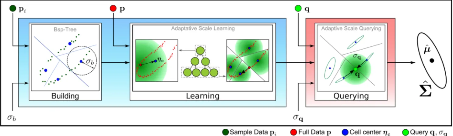
Figure 1. Pipeline: To fix ideas, we illustrate the different steps of our algorithm when the two sets {pi} = {fi} Our CovTree is based on tree main steps : (a) from a sampled data set, we build a binary tree structure from a space partionning of S based on {pi} up to a cell size σb, (b) each node learns the local statistical distribution modeled by an anisotropic kernel by streaming data points through the tree by considering the piand summing a weighted contribution of fito all traversed’ nodes kernel, (c) for any query point q ∈ S and scale σq∈ R, our CovTree models the local distribution of learned data at q at the scale σqby providing a multivariate Gaussian distribution defined from a mean ˆµ and a covariance matrix ˆΣ.
2. fast local distribution estimate, at different scales, without recomputing the data structure;
3. genericity, allowing to solve a number of 2D and 3D processing problems by instantiating our structure with specific spatial and range domains, which includes Non-Local Bayes filtering, data-driven image denois-ing, image holes completion and 3D Non-Local Point Set Surface reconstruction.
3. The Covariance Tree
Assume that we want to restore a data point f ∈ R that is either noisy or incomplete in some way. We also have access to q ∈ S which is related to f in the following man-ner: the prior distribution of f given q can be modelled as a multivariate Gaussian N (µq, Σq) with parameters varying smoothly as a function of q.2
If we know the mapping q 7→ (µq, Σq), and the degra-dation model (given as the conditional probability of the degraded or incomplete ˜f given the clean f ) then we can use standard Bayesian techniques (such as MAP or EAP) to estimate f from the degraded pair (q, ˜f ). In general such a mapping is unknown, but we can estimate it from a large database of examples (pi, fi) ∈ ˆR × ˆS ⊂ R × S, by
aver-2 Note that if this assumption holds, then the data f
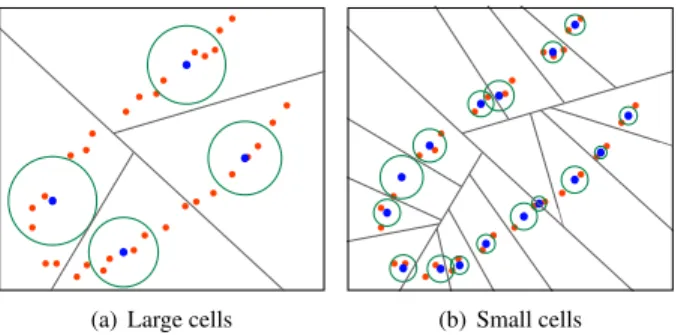
i will be more compactly represented by multivariate Gaussians than by simpler isotropic ones (see Figure 2). Indeed, by using isotropic Gaussian we consider that f is propagating the same way in every direction of the space defining smaller and more numerous cells and decreasing the quality of the learn-ing.
aging a sufficiently large number of neighbours : µq,σq = X pi∈ ˆR φσq(kpi− qk)fi Σq,σq = X pi∈ ˆR φσq(kpi− qk)¯fifi¯T (3)
where ¯fi = (fi− µq,σq). A small scale parameter σq
pro-vides a better localized prior, but larger values are often re-quired to provide a statistically significant estimation of the local Gaussian distribution from the given examples, espe-cially when the dimensions dS and dR are large, as is the case in non-local patch-based filtering or restoration for in-stance.
Unfortunately, high-dimensional restoration problems require large example databases and a brute-force approach to the computation of Eq. (3) at each query point q is un-tractable. We tackle this problem by introducing an hier-archical data structure which summarizes and indexes the database at multiple scales, with a limited amount of mem-ory. This structure is equipped with a fast query mecanism providing an approximation to (3), for any query point q and for a large range of scales σq. Our basic idea is to model the database as an hierarchical set of anisotropic multivari-ate Gaussians approximating smoothly and progressively the distribution of {fi} in the database. At each level of the structure, the kernels are formed by the mean and the co-variance of the local distribution. Consequently, we name our structure Covariance Tree (or cov-tree).
More precisely, a cov-tree is a Binary Space Partition Tree [6] (bsp-tree) carrying anisotropic Gaussians learned from data on its nodes. It defines a rotation-invariant tes-sellation of S into space cells, as well as an hierarchical
(a) Large cells (b) Small cells
Figure 2. Distribution models: Local isotropic Gaussians are too poor a model for manifolds. At a given scale, the balls are too coarse to describe local variations (a). The only solution is to re-fine the partition (b) increasing the number of representative cells.
partition allowing to approximate the database at different scales.
Our approach (as summarized in Figure 1) is essentially based on three operators:
building we perform a top-down hierarchical space par-titioning of S based on {pi} up to a cell size σb, resulting in a binary tree structure for which each node will later carry an anisotropic kernel modeling the local statistical distribu-tion of {fi} in its related space cell (Sec. 3.1);
learning we learn this distribution by streaming (train-ing) data points through the tree, classifying them using pi and summing a weighted contribution of fito all traversed nodes’ kernels (Sec. 3.2);
querying for any query point q ∈ S and scale σq∈ R, our cov-tree provides a multivariate Gaussian distribution, in the form a mean ˆµ and a covariance matrix ˆΣ interpo-lated at q and modelling the distribution of learned data at scale σq(Sec. 3.3).
The two parameters σband σq(that determine the local-ity of learning resp. query) are set to ensure a reasonable ap-proximation of equation (3). Usually, σbis defined smaller than the noise level σn of the training data and σq ' σn. Indeed, given the noise in the data, values σqfiner than the noise σn provide too poor statistical estimate of ( ˆµ, ˆΣ) . The result of the successive steps of building, learning and querying approximates the estimation of covariance matri-ces with a Gaussian kernel of size√2σq.
3.1. Building the tree
Instead of using a kd-tree [2], which fails at capturing anisotropy accurately (see Fig. 3(a)), we give to our cov-tree a bsp structure based on the direction of maximum variation of the input points. Let us consider a tree node η and its associated set of points pj. We compute and store in η a splitting plane {ηd, ηc}, with its normal ηd de-fined as the normalized eigenvector associated to the largest eigenvalue of the covariance of {pj} and its center ηc de-fined as the average of the pj. The cell radius is given
(a) Kd-tree (b) Bsp-tree
Figure 3. Tree structure. A Kd-tree (a) defines partitions of S independantly of the anisotropy of the data. A bsp-tree (b) allows to be rotation-invariant and better model distributions, diminishing the error of the estimated multivariate Gaussian.
by ηr = max pj
kpj− ηck. We then subdivide {pj} into two distinct sets based on their signed distance to the plane (pj− ηc)tηd. Finally, we construct the two children of η based on these two sets. Starting from the root and the entire input {pi}, we perform this recursive construction while ηr > σb. Consequently, our approach is output-sensitive and well adapted to large data sets, the memory footprint of the cov-tree depending only on the desired precision σb.
3.2. Learning local distributions
Once the tree structure is initialized, we can compute the statistics of its cells by streaming pairs of training data point {pi, fi} through it. Starting from the root node, a pair is classified top-down using piand enriches each traversed node η by summing fito its local distribution using a weight widefined from a Gaussian φηr centered at ηc:
µη:= µη+ wifi Ση:= Ση+ wifitfi
(4)
Each point we stream during the learning step increases the precision of our cov-tree without adding additional nodes (i.e., constant memory cost). For a large database, the tree nodes’kernels are typically learned over the full data while the tree’s structure is built from a subset only. Inter-estingly enough, the dataset used for the building step can be different from the learning one.
3.3. Querying local distributions
Once fully built, the tree can be queried using any q ∈ S, providing an anisotropic Gaussian describing the distribu-tion of the learned values around q at scale σq. To do so, we first collect a set of tree nodes in the vicinity of q, at differ-ent scales, by traversing the tree top-down, gathering every node η intersecting the [q, σq] ball and being either a leaf or verifying ηr > σq. Traversing the tree to a finer precision level ηr<< σqwould increases the precision, but increases significantly the computational cost (see Fig 4). Second,
Figure 4. Our fast query limits the number of cov-tree nodes gathered (in green) to reconstruct a local anisotropic distribution. (a)When the requested scale σqis large, only the top nodes are retained. (b) As σqgets smaller, the gathering shaft gets thinner, collecting deeper nodes mostly.
we estimate the distribution at q as a weighted combina-tion of the gathered nodes’ distribucombina-tions, using weights wi defined from a Gaussian φσq centered on q :
ˆ µ = 1 ˆ w X i wiµηi ˆ Σ = 1 ˆ w2 X i wiΣηi− ˆw ˆµ t ˆ µ (5)
Where ˆw and ˆw2are two normalization values.
3.4. Complexity Analysis
We recall that S is the dS-dimensional spatial do-main and R is the dR-dimensional range dodo-main. Each of the Nb points used during the building step appears only once in the Kb cov-tree clusters, resulting in a building cost of O(dSNblog(Kb)). Using Nl points to learn the nodes’statistics, classifying them has a cost of O(NldSlog(Kb)) and learning variations in all nodes has a cost of O(Nllog(Kb)d2R), resulting in a learning cost of O(Nllog(Kb)(dS + d2R)). When querying Nq points, gathering the lists of Kq contributing nodes has a cost of O(NqdSKq); the additional anisotropic Gaussian es-timation (O(NqKqd2
R)) leads to a total querying cost of O(NqKq(dS + d2R)). Last, the memory cost of our cov-tree is O(NbKbd2
R) and remains constant during the online steps (learning and querying), allowing to re-learn and/or reuse numerous times a cov-tree precomputed once.
4. Applications
We provide a few example applications of our cov-tree to solve inverse problems in 2D imaging and 3D rendering. Whenever possible the results are compared with state of the art techniques for the same problems.
The performance numbers reported in this paper were measured on a 2.4 GHz Intel Xeon processor with 12 GB of memory and 8 cores, but running a non-optimized C++
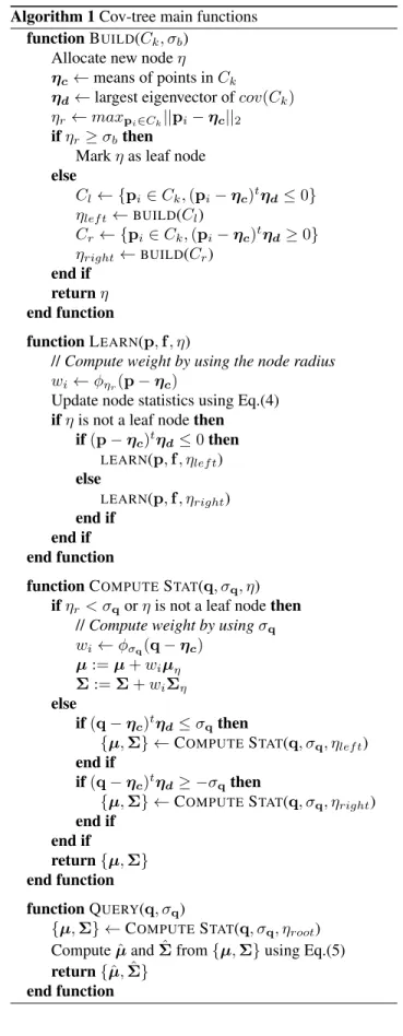
Algorithm 1 Cov-tree main functions function BUILD(Ck, σb)
Allocate new node η ηc← means of points in Ck
ηd← largest eigenvector of cov(Ck) ηr← maxpi∈Ck||pi− ηc||2
if ηr≥ σbthen Mark η as leaf node else Cl← {pi∈ Ck, (pi− ηc)tηd≤ 0} ηlef t←BUILD(Cl) Cr← {pi∈ Ck, (pi− ηc)tηd≥ 0} ηright←BUILD(Cr) end if return η end function function LEARN(p, f , η)
// Compute weight by using the node radius wi← φηr(p − ηc)
Update node statistics using Eq.(4) if η is not a leaf node then
if (p − ηc)tηd ≤ 0 then LEARN(p, f , ηlef t) else LEARN(p, f , ηright) end if end if end function
function COMPUTESTAT(q, σq, η) if ηr< σqor η is not a leaf node then
// Compute weight by using σq wi← φσq(q − ηc)
µ := µ + wiµη Σ := Σ + wiΣη else
if (q − ηc)tηd≤ σqthen
{µ, Σ} ← COMPUTESTAT(q, σq, ηlef t) end if
if (q − ηc)tηd≥ −σqthen
{µ, Σ} ← COMPUTESTAT(q, σq, ηright) end if
end if
return {µ, Σ} end function
function QUERY(q, σq)
{µ, Σ} ← COMPUTESTAT(q, σq, ηroot) Compute ˆµ and ˆΣ from {µ, Σ} using Eq.(5) return { ˆµ, ˆΣ}
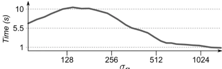
1 5.5 10 128 256 512 1024 T im e (s)
Figure 5. Computation time (in seconds) of 5 · 105queries (ex-cluding the building step which is run only once) of our cov-tree at different scales σq. Time is measured by specifically constraining the use of a single core.
code3which most often takes advantage of only one core.
4.1. Non Local Bayes Filtering
Non-local Bayes denoising [9]4is a bayesian MAP esti-mation from noisy image patches ˜p. 5 The prior multivari-ate Gaussian model for the clean patch is estimmultivari-ated from a neighborhood N˜pof noisy patches, so the estimated co-variance matrix Σ˜pis also corrupted by noise. When we combine the denoising of this covariance matrix with the MAP estimation in equation (2), we obtain the estimated (denoised) patch as ˆ p = µ˜p+ [Σ˜p− σn2Id]Σ −1 ˜ p (˜p − µ˜p) (6) The neighborhood N˜pis not only restricted to patches ˜pi that are close to ˜p in the feature space (R = R3n2 for n × n patches of color images), but also to those associated to nearby pixels (xi, yi). This restriction makes the search for similar patches tractable in very large images, since the search region does not grow with image size. Using the cov-tree, however, we can afford such large search regions without any significant performance penalty.
We propose three variants of NLB denoising which only differ in the choice of the neighborhood N (˜p):
Global Search. The spatial domain S = R = R3n2 is the same as the feature space, so the neighborhood N˜p only depends on ˜p.
Local Search. In order to reproduce the neighborhood of the original NLB we augment the spatial domain with the pixel coordinates (xi, yi), so S = RdS, dS =
3n2+ 2.
Compressed Local Search. As an adaptation of [16] to NLB, we can reduce the spatial domain S to the first
3 The querying process can be parallelized by using one thread for each query. A similar solution can be used for the learning process but care must be taken to avoid concurrent writing to the same cell. Parallelizing the building step is more involved but has less impact since this is the least time-consuming part of the pipeline.
4for simplicity we only consider NLB’s first stage here 5where noise is zero-mean Gaussian with variance σ2
30.7 31 31.3 1 2 4 8 16 32 64 PSNR (dB) Space dimensionality ( )
Figure 6. PSNR (with respect to ground-truth) of NLB denois-ing usdenois-ing our cov-tree with PCA dimensionality reduction in the spatial domain. We measured the PSNRi(dS) on 20 test images i for different values of the spatial dimension dS. The mean curve PSNR(dS) is represented in red and in gray the standard devia-tions of the centered curves PSNRi(dS) − PSNRi. Although the absolute levels of PSNR present a large variation (between 29 and 34 dB) among all images, the shape of the PSNRi(dS) curve as a function of dSis the same for all images and shows a peak around dS= 4 in agreement with the findings of [16] for NLM.
6 principal components in a global PCA analysis of all noisy patches in the image.
Figure 7 presents the denoising results of the original NLB compared to our local variant based on the cov-tree. Our local approach (e) produces better results than the orig-inal NLB (d). We can explain it by our use of the approxi-mate Gaussian kernel φ as a weighting function. In the orig-inal NLB, means and covariance matrices are estimated by averaging the k nearest neighbors with a constant weight. Consequently, covariance matrices can be more strongly af-fected by outliers.
As shown in Figure 6, PCA dimensionality reduction over the S domain not only accelerates the search (as ex-pected), but also produces better performances. The latter can be attributed to the denoising effect of dimensionality reduction, which improves the relevance of the computed neighborhoods N (˜p).
Figure 5 shows that the time required to solve a query in the cov-tree is only mildly affected by the neighborhood size σqof the query. Indeed, as shown in Figure 4, coarse-sized queries explore a lot of nodes in breadth but stop the search at the top of the tree while a fine-sized query explores fewer nodes in breadth but explores the tree in depth. Con-sequently, the number of nodes (and hence the computa-tional complexity) for each radius size is equivalent, except for medium sized queries which involve the largest number of nodes.
4.2. Data Driven Image Denoising
In [11] the use of huge image databases is advocated as a way to learn the prior underlying natural image patches. Their procedure (called shotgun NLM in [10]) was shown to serve as a way to estimate the fundamental limits of non-local image denoising methods, but no attempt was done to make the computation time actually tractable for real
appli-PSNR 14.7 dB
(a) Original (b) Noise std. dev. 0.2
PSNR 28.3 dB
(c) Accelerated NLM (6+2-D)
PSNR 28.9 dB
(d) NLB original (147+2-D)
PSNR 29.2 dB
(e) Our filter (6+2-D) Figure 7. Non-local filtering: We use our CovTree to learn 7 × 7 RGB patches extracted from the noisy image (b). The original patch dimensionality (147-D) is reduced to 6-D using PCA as suggested for NLM by [16]. When compared to an accelerated implementation of NLM [7] (c) or the original NLB (d), our filter (e) better recovers features thanks to the use of an approximate Gaussian kernel φ.
(b) Noise
(a) Original (d) Our NLB
(147+2-D) (e) Data-driven NLB (147-D) (c) NLB original (147+2-D) PSNR 30.2 dB PSNR 31.1 dB PSNR 30.0 dB PSNR 22.4 dB
Figure 8. Data driven image denoising: We use our CovTree to learn from about 108 clean 7 × 7 RGB patches extracted from an image database (first line) to denoise an image corrupted by a noise of standard deviation of 0.1 (b) by exploiting the prior underlying natural images. Compared to the original image (a), our data driven filter (e) better preserves features than using the original NLB filter (c) or our single-image CovTree-NLB filter (d).
cations. A similar idea was proposed in [19] for a PLE-like algorithm with 200 Gaussians, thus requiring many days to learn the prior on a largedatabase. In this section we ap-ply the same idea to implement a ”shotgun NLB” denois-ing algorithm, but usdenois-ing the cov-tree to make both learndenois-ing and restoration computationally tractable with large learn-ing databases.
Indeed, we propose to use an external noiseless image database instead of noisy patches to denoise a noisy im-age. This idea has two main benefits: we can increase the number of learned patches (without a significant penalty in computation time or memory use) and data is not de-graded by noise, thus increasing the precision of the esti-mated anisotropic Gaussian.
In practice, we build the tree at a scale σb= σnby con-sidering the colored noised patches (without the pixel coor-dinate) to fix the hierarchy of spatial domain cells. Then, we learn the corresponding range-domain Gaussian
mod-els from the database of noiseless colored patches. Finally, the covariance matrix Σ˜pand the mean vector µp˜ are es-timated from a noisy patch ˜p with σq = σn. In contrast to the previous section, the estimated anisotropic gaussians N (µ˜p, Σ˜p) are noiseless, consequently, we applied equa-tion (2) directly, without need for denoising the covariance matrix.
Figure 8 shows our result of denoising an image of a fac¸ade using a database of noiseless images of similar fac¸ades in the same city (but not the same fac¸ade). As expected, the database-driven denoising performs better. More extensive experimentation is needed to check if this reconstruction is actually close to the fundamental limits announced in [11] .
Our database contains about 108patches and the learning phase takes about 5 hours and 8GB of RAM to hold the data-structure. This is several orders of magnitude faster than the times reported in [11, 19], while our database is also larger. Reconstruction takes about 5 minutes.
4.3. Reconstruction from random samples
One of the most visually striking applications of Bayesian MAP estimation with a Gaussian mixture prior model for image patches, is the reconstruction of an image, from a small random subset of its pixels (20% in our case), as showcased in [18] among others. Let’s consider a patch q sampled by a known random sampling operator ˜q = Sq. As before, we consider that image patches are locally mod-eled as an anisotropic Gaussian distribution, with mean µ˜q and covariance Σ˜qestimated from the local dictionary. We assume that ˆq0is an initial estimate of the complete patch ( obtained by a cubic interpolation over the Delaunay tri-angulation). This patch serves as a query to extract a local statistical prior for q from the cov-tree. Then by Bayesian
(a) Original (b) Masked (c) Cubic (d) Our result Figure 9. Data driven reconstruction from sparse samples: We obtain from an original image (a) a masked image by extracting randomly 20% of the original pixels (b). By learning about 108 patches with our CovTree, we reconstruct an image (d) by apply-ing Eq. (7) with a coarse-to-fine query scales, and startapply-ing from a cubic interpolation (c).
MAP estimation, we write the recovered patch ˆqias :
ˆ qi+1 = (ΣˆqiS HS +σi2 2 Id) −1(Σˆ qiS Hq +˜ σ2i 2 µˆqi) (7)
Combining all reconstructed patches by aggregation, we ob-tain a first reconstruction I1from the interpolated image I0. The patches ˆqi in this first reconstruction (i = 1) can in turn be used as an initialisation/query to obtain more accu-rate prior and reconstruction ˆqi+1. We iterate the process with until ˆqi equals ˆqi+1 by using a coarse-to-fine query scale σi = αiσ0where α ∈ [0, 1] is a scale factor. Figure 9 presents the result of our approach over an image were only 20% random samples were retained. In our experiments α = 0.8 and σ0= 0.65
5. Conclusion and perspectives
We proposed a novel data structure and associated algo-rithms that allow to deal with a continuous family of local multivariate Gaussian models: both efficient learning over a large database and fast queriyng are supported. The ex-tracted model varies continuously over a range domain R when the query point varies over a (possibly different) spa-tial domain S, and different scale levels can be specified by the query resulting in various degrees of spatial locality of the extracted statistical model.
The relevance of such a data structure is motivated by image restoration problems via Bayesian MAP with local Gaussian priors on the image patches. Such models became incresingly sucessful in image processing during the last 5 years, because they are very close to an accurate statistical model of natural images. However, progress in this area has been slow because we lack the required tools for efficiently handling the massive amounts of data that need to be fed to learn these models in order to approach optimal results. The cov-tree is an attempt to fill this gap.
Given the genericity of the cov-tree, its applicability reaches potentially far beyond image restoration. In the supplementary material we include an application that im-proves an NLM-like algorithm for denoising and interpola-tion of 3D point clouds [8]. In this case a data structure is definitely required to index and query a set of patches even for point cloud of 106points. The reason is that common ac-celeration and search techniques that are used by non-local methods in 2D image processing do not apply to irregular 3D point sets over a surface that has no implicit parameter-ization.
Acklowedgements This work has been partially funded by the EC under contracts FP7-287723 REVERIE, FP7-323567 HAR-VEST4D, by the French government under ANR iSpace&Time, FUI CEDCA and CNES R&T 128435 projects.
References
[1] A. Adams, J. Baek, and M. A. Davis. Fast high-dimensional filtering using the permutohedral lattice. In CGF, volume 29, pages 753–762, 2010.
[2] A. Adams, N. Gelfand, J. Dolson, and M. Levoy. Gaussian kd-trees for fast high-dimensional filtering. TOG, 28(3):21, 2009.
[3] V. Aurich and J. Weule. Non-linear gaussian filters perform-ing edge preservperform-ing diffusion. In Mustererkennung 1995, pages 538–545. 1995.
[4] S. Awate and R. Whitaker. Higher-order image statistics for unsupervised, information-theoretic, adaptive, image filter-ing. In CVPR, volume 2, pages 44–51, 2005.
[5] A. Buades, B. Coll, and J.-M. Morel. A non-local algorithm for image denoising. In CVPR, volume 2, pages 60–65, 2005. [6] H. Fuchs, Z. M. Kedem, and B. F. Naylor. On visible sur-face generation by a priori tree structures. In SIGGRAPH, volume 14, pages 124–133, 1980.
[7] E. S. Gastal and M. M. Oliveira. Adaptive manifolds for real-time high-dimensional filtering. TOG, 31(4):33, 2012. [8] T. Guillemot, A. Almansa, and T. Boubekeur. Non local
point set surfaces. In 3DIMPVT, pages 324–331, 2012. [9] M. Lebrun, A. Buades, and J.-M. Morel. Implementation of
the ”Non-Local Bayes” Image Denoising Algorithm. IPOL, 2013:1–42, 2013.
[10] M. Lebrun, M. Colom, A. Buades, and J. Morel. Secrets of image denoising cuisine. Acta Numerica, 21:475–576, 2012. [11] A. Levin and B. Nadler. Natural image denoising: Optimal-ity and inherent bounds. In CVPR, pages 2833–2840, 2011. [12] J. Mairal, F. Bach, J. Ponce, G. Sapiro, and A. Zisserman.
Non-local sparse models for image restoration. In ICCV, pages 2272–2279, 2009.
[13] G. Motta, E. Ordentlich, I. Ramirez, G. Seroussi, and M. J. Weinberger. The dude framework for continuous tone image denoising. In ICIP, volume 3, pages III–345, 2005. [14] S. Paris and F. Durand. A fast approximation of the bilateral
filter using a signal processing approach. IJCV, 81(1):24–52, 2009.
[15] S. M. Smith and J. M. Brady. Susan—a new approach to low level image processing. IJCV, 23(1):45–78, 1997.
[16] T. Tasdizen. Principal components for non-local means im-age denoising. In ICIP, pim-ages 1728–1731, 2008.
[17] C. Tomasi and R. Manduchi. Bilateral filtering for gray and color images. In ICCV, pages 839–846, 1998.
[18] G. Yu, G. Sapiro, and S. Mallat. Solving inverse prob-lems with piecewise linear estimators: from gaussian mix-ture models to strucmix-tured sparsity. TIP, 21(5):2481–2499, 2012.
[19] D. Zoran and Y. Weiss. From learning models of natural image patches to whole image restoration. In ICCV, pages 479–486, 2011.