Finite element simulation of the critically refracted longitudinal wave in a solid medium

HAL Id: hal-00538341

https://hal.archives-ouvertes.fr/hal-00538341

Submitted on 22 Nov 2010

HAL is a multi-disciplinary open access

archive for the deposit and dissemination of sci-entific research documents, whether they are pub-lished or not. The documents may come from teaching and research institutions in France or abroad, or from public or private research centers.

L’archive ouverte pluridisciplinaire HAL, est destinée au dépôt et à la diffusion de documents scientifiques de niveau recherche, publiés ou non, émanant des établissements d’enseignement et de recherche français ou étrangers, des laboratoires publics ou privés.

Finite element simulation of the critically refracted

longitudinal wave in a solid medium

Weina Ke, Salim Chaki

To cite this version:

Weina Ke, Salim Chaki. Finite element simulation of the critically refracted longitudinal wave in a solid medium. 10ème Congrès Français d’Acoustique, Apr 2010, Lyon, France. �hal-00538341�

10ème Congrès Français d'Acoustique

Lyon, 12-16 Avril 2010

Finite element simulation of the critically refracted longitudinal

wave in a solid medium

Weina Ke, Salim Chaki

Ecole des Mines de Douai, 941 rue Charles Bourseul, F-59508 Douai Cedex, {ke,chaki}@ensm-douai.fr

At critical incidence, the critically refracted longitudinal (LCR) wave propagating in the subsurface domain of a solid specimen can be used in numerous non-destructive testing (NDT) applications, such as characterization of surface geometric aspects or structural subsurface properties of materials, like residual stress measurement. Generally speaking, LCR wave has bigger penetration depth, which may change with driven frequency and incident angle. This communication paper deals with the study of LCR beam profile using numerical tools based on Finite Element (FE) method. The simulations are performed in time and frequency domain in the case of elastic, homogenous and isotropic material. For the simulations in frequency domain, Fourier transform is applied to separate the different spectrum components. All results showed the composition of this acoustical field, as well as certain special characteristics.

1 Introduction

The critically refracted longitudinal wave, which is generated with ultrasound wave incident at the first critical angle for longitudinal wave, propagates along the surface of specimens, thus reflects surface and subsurface characteristics by the wave properties linked to material elasticity or signals due to interaction between waves and defects. At the other side, very often, Rayleigh waves are employed for the NDT applications of surface characterization or subsurface breaking cracks detection. They are easily excited and only weakly attenuated along more or less "perfect" surfaces, but the disadvantage of being very sensitive to surface roughness, as well as exponential decay within a few wavelengths normal to the surface, prevents quantitative characterization of larger cracks. In contrast to that, the big angle beam probe, typically LCR wave, which is applied according to Snell-Descartes law with longitudinal wave critically refracted and propagating along surface through subsurface area, has more uniform behaviour even in anisotropic materials and thus probably benefits the NDT applications.

The analytical solution of LCR is first provided by L. V. Basatskaya for a simplified 2D case [1], and then carried on with more detailed discuss about the nature of the LCR by K. J. Langenberg [2], while the experimental characterization of beam profile is reported in Ref [3]; besides, the applications of this technique are mostly studied by D. E. Bray et al in the domain of residual stress evaluation [4]-[9].

Generally speaking, the observed propagating wave-front has following features: longitudinal wave speed, strong decay on the surface within a few centimetres, main beam of approximate 74° in steel, accompanied by a bulk 33° shear wave. According to the previous researches, the penetration depth of the beam in the subsurface area is mainly depend on the driven frequency; nevertheless, the incident angle might also have effect on it, as well as on the propagation distance.

To reproduce the classical numerical results for better understanding the characteristics of the LCR beams, as well

as to set the available models for future optimization for the inspection results, the LCR ultrasonic technique for material characterization is here studied theoretically. In this paper, the basic modelling results are introduced by modelling the

ultrasonic LCR beam characteristics in isotropic

homogenous material both in time and frequency domain.

2 Numerical studies

Sample i θ θr 1 x 2 x 3 x 1 x 2 x 3 x

Figure 1: Schematic of angle beam probe technique The presented modelling are all realized using commercial soft ware based on Finite Element method [10]. The models are set as two dimensional with u3=0 to model the cases of bulk longitudinal and transversal waves. The illustration for this specified case with corresponding

coordinate system is as shown in Figure 1, where x2

direction is normal to the media surface, x1 direction parallel to the surface along the wave propagation direction, and, θi and θr in the figure are incident and refracted angle,

respectively. The modelled media is chosen as steel with properties as shown in Table 1.

Density ρ (g/cm3₎ Young’s _modulus E (GPa) Poisson ratio ν Wave velocity (m/s) Longitudinal Transversal 7.8 210 _0.29 5940 3230

2.1 Modelling in time domain

The acoustical field is obtained by solving the motion equation: 2 2 2 t u x x u C i k j l ijkl _∂ ∂ = ∂ ∂ ∂ _ρ 3 , 2 , 1 , , ,jk l= i (1)

where u is the displacement vector of local particle, Cijkl is

the material stiffness tensor, ρ is the density; while for isotropic materials with independent Lamé constants λ and μ, it can be rewritten as:

(

)

2 2 2 2 2 t u x u x x u _i j i i j j ∂ ∂ = ∂ ∂ + ∂ ∂ ∂ +μ μ ρ λ i,j,k,l=1,2,3 (2) -a O a 1 x 2 x 1 x 2 x c i θ θ ≈

Figure 2 Schematic for excitation condition. For two dimensionally simulations, to have longitudinal wave propagating in x1 direction, the excitation can be defined as the following boundary condition:

( )

⎩ ⎨ ⎧ = 0 22 t f σ 0 21= σ a x a x > ≤ ∞ < x (3) While the applied transient signal can be defined as below:

where α is a parameter controlling the pulse width, t0 is the pulse delay time, and ωc=2πfc, where fc is the center

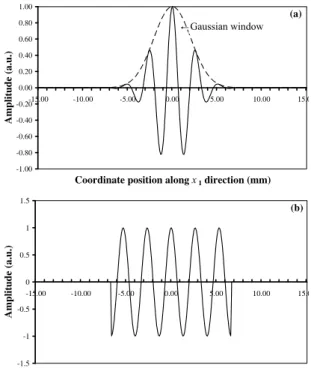
frequency of the pulse. The sample of generated signal is as shown in Figure 3 (a) with α=1.5, t0=6 μs, fc=1.0 MHz, and

Figure 3 (b) shows the corresponding frequency spectrum of the signal. -0.5 -0.4 -0.3 -0.2 -0.1 0 0.1 0.2 0.3 0.4 0.5 0.0 1.0 2.0 3.0 4.0 5.0 6.0 7.0 8.0 9.0 10.0 11.0 Times (μs) A m plitud e (a. u.) (a) 0.0 0.2 0.4 0.6 0.8 1.0 1.2 1.4 1.6 1.8 2.0 0.0 0.3 0.7 1.0 1.4 1.7 2.1 2.4 2.7 Frequency (MHz) A m pl it ud e ( a.u .) (b)

Figure 3(a) Sample of generated transient signal with α=1.5, t0=6μs, fc=1.0 MHz;(b) Corresponding frequency

spectrum.

So as far as to generate LCR wave, the exact excitation can be defined as:

( )

t

(

t t

)

(

i

(

kx t

)

)

f _α ωc ωc π α ⎟⎟⎠ − ⎞ ⎜ ⎜ ⎝ ⎛ ₋ − = exp 2 exp 2 2 2 2 0 , (5) where k’ is the wave number in the incident medium, θ is the incident angle, and k=k’sinθ is the corresponding longitudinal wave-number in refracted medium along x1 direction, in this way, the variable incident angle is introduced into the modelling. The excitation is defined on the upper surface under the coordinate system as shown in Figure 2 within the regionx ≤ . a

Corresponding to the central driven frequency f=2.25 MHz, the wavelengths of longitudinal and transversal waves are 2.64 mm and 1.44 mm, respectively; and for second-order quadratic elements, the mesh is required to satisfy at least 3 or 4 elements within one wavelength.

The result showed in Figure 4 corresponds to a 70×50 mm2 _{model with the range of x}

1 from -20 mm to 50 mm and

x2 from 0 mm to 50 mm, with a=10 mm. It is represented as

distribution of displacement amplitude 2

2 2

1 u

u + at time

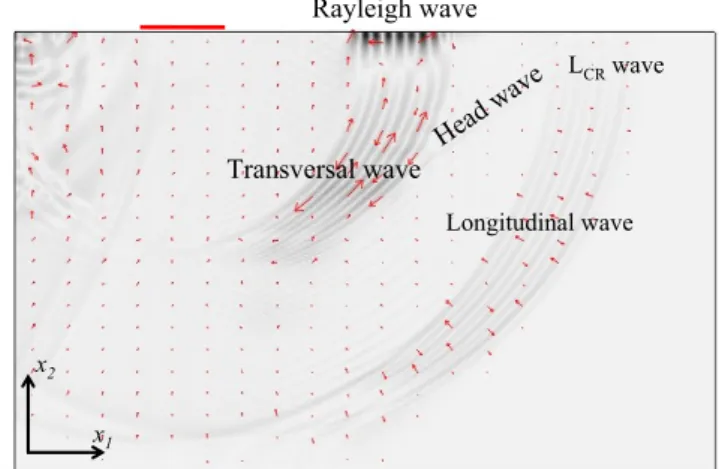
t=8 μs. The gray panel color is related to the amplitude of the solution, while the red arrow is related to the displacement vector. Based on this latter, it is possible to distinguish different wave components propagating in this

solid medium. The first arrived are LCR wave with

displacement parallel to the propagation direction and longitudinal wave with displacement perpendicular to its wave-front, followed by head wave remarked with a plane wave-front and finally the transversal wave, whose displacement is parallel to its wave-front, and Rayleigh wave. Besides, the transversal wave is overlapped with surface wave in the subsurface region which can be distinguished from the wave-length [11].

Longitudinal wave Rayleigh wave Head wave Transversal wave x1 x2 LCRwave Longitudinal wave Rayleigh wave Head wave Transversal wave x1 x2 LCRwave

Figure 4: Predicted results of distribution of displacement amplitude with transient excitation at t=8μs. But as shown in the results in time domain, it is not so convenient to trace the displacement amplitude due to the adjacent different-shaped wave-front, while the simulation results in frequency domain can offer with easy access to the characterization of beam profile.

2.2 Modelling in frequency domain

Simulation in time domain is not enough efficient due to the limit from number of degrees of freedom and numerous time steps. Modeling is now carried on in frequency domain to improve all these shortages based on the Fourier transform of equation (1).

( )

t

(

t t

)

(

i t

)

f ω_c ω_c α π α ⎟⎟⎠ − ⎞ ⎜ ⎜ ⎝ ⎛ − − = exp 2 exp 2 2 2 2 0 , (4)

Sample Emitter Ultrasound x₁ x₂ Sample Emitter Ultrasound Sample Emitter Ultrasound Sample Emitter Ultrasound x₁ x₂ x₁ x₂ x₁ x₂

Figure 5: Periodical distribution of excitation condition loaded on boundary.

The excitation loaded on top surface boundary, as shown in Figure 5, corresponds to the Fourier transform of harmonic excitation in time domain. This excitation condition is independent of time variable t, but changes

periodically with spatial variable x1, which is also

coincident with Snell’s law concerning the relative wave-number k.

Figure 6: Model setup for simulation in frequency domain. The model is as shown in Figure 6 corresponding to stationary case with harmonic excitation, which can be set on the boundary as a spatial periodical distribution and can be modulated by a Gaussian window (see Figure 7a) and expressed as

( )

(

1

)

2 0 1 _exp 2 20 exp ikx a x x x f _⎟⎟ − ⎠ ⎞ ⎜ ⎜ ⎝ ⎛ ⎟ ⎠ ⎞ ⎜ ⎝ ⎛ − − = , (6)

where x0 is the midpoint of the excitation zone, while k and

a are the same denotations as before. As shown in the

figure, absorbing regions are set around in front of the three boundaries except the one with excitation [12]-[14], for example, for the right end of the propagation domain, the absorbing region can be set with material elastic coefficients Cij as:

(

)

(

)

3 a r ij ij AR ij C iC x x L C = + − , x1>xr. (7)

where La is the length of the absorbing region, x1=xr is the

interface between propagation domain and right-side absorbing region.

The medium is also set to be steel with the material properties as shown in Table 1. With a driven frequency of 2.25 MHz, the model is set to be 80×50 mm2 _{with the range} of x1 from -20 mm to 60 mm and x2 from 0 mm to 50 mm. The excitation is set on the top boundary centered at x1=0 with a width of 2a=5λl, λl is the longitudinal wavelength, as

shown in Figure 7(a). The obtained displacement results appear as superposition of longitudinal and transversal components as shown in Figure 8.

-1.00 -0.80 -0.60 -0.40 -0.20 0.00 0.20 0.40 0.60 0.80 1.00 -15.00 -10.00 -5.00 0.00 5.00 10.00 15.0

Coordinate position along x1 direction (mm)

Amplit ude ( a.u.) (a) Gaussian window -1.5 -1 -0.5 0 0.5 1 1.5 -15.00 -10.00 -5.00 0.00 5.00 10.00 15.0

Coordinate position along x1 direction (mm)

Amplit

ude

(

a.u.)

(b)

Figure 7: Excitation applied on the boundary for simulation in frequency domain, (a) with Gaussian window; (b)

without Gaussian window.

Figure 8: Distribution of u2 displacement component

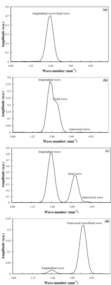
obtained in frequency domain at f=2.25 MHz with critically incident excitation modified with Gaussian window. So in order to separate and characterize directivities of different wave components, Fourier transform is applied to obtain the amplitudes of different components with wave-number frequency spectrum at given refracted angles. The signals used for Fourier transform to obtain the frequency spectrum are actually picked up from simulation results by monitoring displacement between propagation distance 10 mm and 40 mm along each refraction angle θr as shown in Figure 9, and the results of Fourier transform are as shown in Figure 10. By this way, it is possible to obtain the amplitudes of different wave components in different refraction angles for directivity. As the phase velocity of longitudinal wave, transversal wave and surface wave in steel are 5940 m/s, 3230 m/s and 2996 m/s respectively, so at this driven frequency, the corresponding wave-number are 2.38 mm-1_{, 4.37 mm}-1 _{and 4.72 mm}-1_{, respectively.}

In this case, in the direction of θr=90°, only the components with the wave-number of longitudinal wave exists, which may represent LCR wave and head wave. As illustrated in Figure 11, the projection of wave-number of

head wave on this direction is exactly equal to the one of longitudinal wave. -0.6 -0.4 -0.2 0 0.2 0.4 0.6 0.8 10 15 20 25 30 35 40 Propagation distance (mm) Displa ce me nt (a.u .) (a) -0.25 -0.2 -0.15 -0.1 -0.05 0 0.05 0.1 0.15 0.2 10 15 20 25 30 35 40 Propagation distance (mm) D ispl acement ( a.u. ) (b) -0.8 -0.6 -0.4 -0.2 0 0.2 0.4 0.6 0.8 10 15 20 25 30 35 40 Propagation Distance (mm) Displa cemen t (a.u.) (c) -0.3 -0.25 -0.2 -0.15 -0.1 -0.05 0 0.05 0.1 0.15 0.2 0.25 10 15 20 25 30 35 40 Propagation distance (mm) D isp lace men t ( a.u .) (d)

Figure 9: Real part of displacement monitored in different refracted directions from result of Figure 8: (a) θr=90°, (b)

θr=85°, (c) θr=62° (d) θr=33°. 0 0.1 0.2 0.3 0.4 0.5 0.6 0.00 1.23 2.46 3.69 4.92 Wave-number (mm-1₎ Ampli tude (a. u.) (a)

longitudinal wave/ head wave

0 0.05 0.1 0.15 0.2 0.25 0.3 0.35 0.4 0.00 1.23 2.46 3.69 4.92 Wave-number (mm-1₎ Amplit ude (a .u.) (b) longitudinal wave head wave transversal wave 0 0.1 0.2 0.3 0.4 0.5 0.6 0.7 0.8 0.9 0.00 1.23 2.46 3.69 4.92 Wave-number (mm-1₎ Ampl itude (a. u.) (c) longitudinal wave transversal wave head wave 0 0.05 0.1 0.15 0.2 0.25 0.00 1.23 2.46 3.69 4.92 Wave-number (mm-1) Ampl itude (a. u.) (d)

transversal wave/head wave

longitudinal wave

Figure 10: Frequency spectrums obtained at different refracted angles based on the result obtained with excitation

with Gaussian window: (a) θr=90°, (b) θr=85°, (c) θr=62° (d) θr=33°.

λ θ λ/sinθ 2 x k 1 x k k 2 x k 1 x k k x1 x2 Propagation direction

Figure 11: Projection of the wave-number related to the periodicity of wavelength

While as the refraction angle becomes smaller, the head-wave component go apart from that of longitudinal head-wave as shown in Figure 10 (b) and (c), and finally overlapped with that of transversal wave at θr=33° as shown in Figure 10 (d). The obtained directivity of longitudinal components is as shown in Figure 12, and the maximum lobe related to Figure 10 (c) is located at θr=62°.

Attention is recalled to pay to distortion due to the superposition of longitudinal wave and head-wave in the near-surface region, in this case, the separation of these two

waves can be achieved by using the u2 displacement

component, which is just included in head-wave.

0.2 0.4 0.6 0.8 1 0 30 60 90 0.2 0.4 0.6 0.8 1 0 30 60 90 (a) 0.2 0.4 0.6 0.8 1 0 30 60 90 0.2 0.4 0.6 0.8 1 0 30 60 90 (b) Figure 12: Displacement amplitude of Longitudinal components in different refracted direction generated by excitation: (a) with Gaussian window, (b) without Gaussian

window.

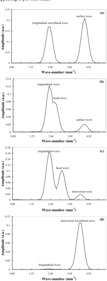
Generally speaking, the characteristics of LCR wave are probably due to the edge effect of excitations [2]. To study this effect, excitation without Gaussian window as illustrated in Figure 7(b) is applied. The obtained simulation results with critically incident longitudinal wave is as shown in Figure 13, and similar frequency spectrum results of separated different wave components for further analyse are plotted in Figure 14.

Figure 13: Distribution of u2 displacement component

obtained at f=2.25 MHz by excitation corresponding to critically incident (27.16°) without Gaussian window.

In this case, by comparison to Figure 10, the mainly difference lays in the appearance of surface wave as shown

in Figure 14 (a) and (b). Directivity of the longitudinal components is also changed for this excitation mode (see Figure 12 (b) with the maximum lobe located at a refracted angle θr=77° as shown in Figure 14 (c), which is the case appearing in previous study.

0 0.05 0.1 0.15 0.2 0.25 0.00 1.23 2.46 3.69 4.92 Wave-number (mm-1₎ A mplit ude ( a. u. ) (a)

longitudinal wave/head wave

surface wave 0 0.02 0.04 0.06 0.08 0.1 0.12 0.14 0.00 1.23 2.46 3.69 4.92 Wave-number (mm-1) A m plitud e (a.u .) (b) longitudinal wave head wave surface wave 0 0.02 0.04 0.06 0.08 0.1 0.12 0.14 0.16 0.18 0.00 1.23 2.46 3.69 4.92 Wave-number (mm-1₎ A mplit ude (a. u. ) (c) longitudinal wave head wave transversal wave 0 0.02 0.04 0.06 0.08 0.1 0.12 0.00 1.23 2.46 3.69 4.92 Wave-number (mm-1) A m pl it ud e ( a.u .) (d) longitudinal wave

transversal wave/head wave

Figure 14: Frequency spectrums obtained at different refracted angles based on the result obtained with excitation

without application of Gaussian window: (a) θr=90°, (b) θr=85°, (c) θr=77° (d) θr=33°

3 Conclusion

A numerical simulation was carried out on both time and frequency domains to study the ultrasonic field refracted at longitudinal critically incident angle. The results in time domain show clearly the composition of the acoustical field as LCR wave, main longitudinal wave, head-wave, transversal wave and Rayleigh wave. While the simulation in frequency domain is advantageous to study the energy distribution of different wave components. In his case, all the wave components are overlapped in the propagation domain, but actually can be separated based on different wave-numbers using Fourier transform. The phenomena due to the edge effects of the excitation are demonstrated either as a change in energy distribution or in wave components.

Based on the availability of these numerical results, further works could concern the stress measurement or

subsurface defect detection using LCR wave or main

longitudinal wave respectively.

4 Reference

[1] L. V. Basatskaya, I. N. Ermolov, “Theoretical

analysis of ultrasonic longitudinal undersurface waves in solid medium”, Soviet Journal of

Nondestructive Testing, 16 (7), 524-530 (1981).

[2] K. J. Langenberg, P. Fellenger, R. Marklein, “On the nature of the so-called subsurface longitudinal wave and/or the surface longitudinal 'creeping' wave", Res.

Nondest. Eval., 2, 59-81 (1990).

[3] P. G. Junghans, D. E. Bray, “Beam characteristics of high angle longitudinal wave probe”, NDE: Applications, Advanced Methods, and Codes and Standards ASME, PVP-Vol.216/NDE-Vol.9, 39-44 (1991).

[4] D E. Bray, P. Junghans, “Application of the LCR

ultrasonic technique for evaluation of post-weld heat treatment in steel plates”, NDT & E International, 28 (4), 235-242 (1995).

[5] W. Tang, D. E. Bray, “Stress and yielding studies using critical refracted longitudinal wave”, NDE:

Engineering Codes and Standards and Materials Characterization, ASME,

PVP-Vol.322/NDE-Vol.15, 41-48 (1996).

[6] T. Leon-Salamanca, D. E. Bray, “Residual Stress

Measurement in Steel Plates and Welds Using Critically Refracted Longitudinal (LCR) Waves”,

Res. Nondestr. Eval., 7, 169-184 (1996).

[7] D. E. Bray, R. K. Stanley, “Nondestructive

Evaluation: A Tool in Design, Manufacturing, and Service”, Boca Raton, FL: CRC Press (1997). [8] D. E. Bray, W. Tang, "Subsurface stress evaluation

in steel plates and bars using the LCR ultrasonic wave", Nuclear Engineering and Design, 207, 231– 240 (2001).

[9] H. Qozam, S. Chaki, G. Bourse, C. Robin, H.

Walaszek, P. Bouteille, “Microstructure effect on the Lcr elastic wave for welding residual stress measurement”, Experimental Mechanics, 50, 2, 179-185, (2010)

[10] COMSOL, User’s Guide and Introduction. Version 3.5a by – COMSOL, http://www.comsol.com/. [11] W. Hassan, W. Veronesi, “Finite element analysis of

Rayleigh wave interaction with finite-size, surface-breaking cracks”, Ultrasonics, 41, 41–52 (2003). [12] W. Ke, M. Castaings, C. Bacon, 3D Finite Element

simulations of an air-coupled ultrasonic NDT system, NDT & E International, 42 (6), 524-533 (2009).

[13] B. Hosten, M. Castaings, “Finite elements methods for modelling the guided waves propagation in structures with weak interfaces”, J. Acoust. Soc. Am., 117 (3), 2005.

[14] B. Hosten, C. Biateau, “Finite element simulation of the generation and detection by air-coupled transducers of guided waves in viscoelastic and anisotropic materials”, J. Acoust. Soc. Am., 123 (4), 1963-1971 (2008).