Predictive controller considering electrical constraints: a case example for five-phase induction machines

Science Arts & Métiers (SAM)

is an open access repository that collects the work of Arts et Métiers Institute of

Technology researchers and makes it freely available over the web where possible.

This is an author-deposited version published in: https://sam.ensam.eu Handle ID: .http://hdl.handle.net/10985/15436

To cite this version :

Mario BERMÚDEZ, Cristina MARTÍN, Federico BARRERO, Xavier KESTELYN - Predictive controller considering electrical constraints: a case example for fivephase induction machines -IET Electric Power Applications p.12 - 2019

Any correspondence concerning this service should be sent to the repository Administrator : archiveouverte@ensam.eu

1

Predictive controller considering electrical constraints: a case example for

five-phase induction machines

Mario Bermúdez

1,2,*

_{, Cristina Martín}

2

_{, Federico Barrero}

2

_{, Xavier Kestelyn}

1

1 _{Univ. Lille, Arts et Metiers ParisTech, Centrale Lille, HEI, EA 2697 – L2EP – Laboratoire d’Electrotechnique}

et d’Electronique de Puissance, F-59000, Lille, France

2 _{Departamento de Ingeniería Electrónica, Universidad de Sevilla, Camino de los Descubrimientos s/n, 41092,}

Sevilla, Spain

*_{mario.bermudez-guzman@ensam.eu}

Abstract: The modern control of power drives involves the consideration of electrical constraints in the regulator strategy, including voltage/current limits imposed by the power converter and the electrical machine, or magnetic saturation due to the iron core. This issue has been extensively analysed in conventional three-phase drives but rarely studied in multiphase ones, despite the current interest of the multiphase technology in high-power density, wide speed range or fault-tolerant applications. In this paper, a generalised controller using model-based predictive control techniques is introduced. The proposal is based on two cascaded predictive stages. First, a continuous stage generates the optimal stator current reference complying with the electrical limits of the drive to exploit its maximum performance characteristic. Then, a finite-control-set predictive controller regulates the stator current and generates the switching state in the power converter. A five-phase induction machine with concentrated windings is used as modern high-performance drive case example. This is a common multiphase drive that can be considered as a system with two frequency-domain control subspaces, where fundamental and third harmonic currents are orthogonal components involved in the torque production. Experimental results are provided to analyse the proposed controller, where optimal reference currents are generated and steady/transient states are studied.

1. Introduction

The industrial demand of higher requirements in the peak torque and power density of modern motor drives is forcing a large increment in their reliability levels, introducing stringent controllers with the ability of managing failure mechanisms and critical electrical limits. For instance, the switching frequency and the current control limit are considered in [1] to avoid an excessive temperature increment in the critical components of the system. Optimal dq current control vectors are estimated to maximise the drive’s efficiency and speed-torque performance within the temperature and voltage constraints. The flux reference is also evaluated to guarantee the maximum torque capability over the entire speed range of induction [2,3] or permanent magnet [4] machines or, more recently, different controllers are presented and experimentally compared in [5], where permanent magnet synchronous motors are again considered. Most, if not all, of these scientific studies focus on conventional three-phase drives, where one dq reference subspace appears and an analytical expression of the optimal stator current reference that respects the imposed constraints can be easily obtain. The machine flux is usually weakened (the d-current stator component is reduced) to respect the imposed voltage limit, adjusting at the same time the q-current stator component with the aim of not exceeding the current limit.

The situation becomes however much more complex when a multiphase electromechanical drive is considered. The interest in the last two decades of the scientific community in the multiphase (more than three) technology comes from its inherent fault-tolerant capabilities and its ability to manage more power with lower current harmonic

content and lower torque pulsation than conventional three-phase machines [6,7]. Thus, it offers an intrinsic characteristic in the low electrical stress on the machine and power electronic components and an attractive alternative in safety and reliability industrial applications [8]. However, the appearance of multiple orthogonal dq control subspaces involved in the torque production in the multiphase drive highly complicates the extraction of the maximum torque under electrical limits and constraints. Notice that the number of the frequency-domain subspaces in a multiphase machine increases with the number of phases and winding topology (concentrated or distributed windings) [6-8]. Luckily, one of the most interesting case studies from the industrial perspective is the five-phase induction machine (IM) with a distributed or concentrated winding topology, which only duplicates the considered frequency-domain control subspaces compared with the three-phase case. Focusing on five-phase drives, if a distributed winding topology is considered, only the fundamental subspace produces electromagnetic torque, while the third harmonic current components generate losses in the machine and must be limited to avoid undesired performance and harmonics. On the contrary, a concentrated winding topology can increase the torque density using the two frequency-domain subspaces for the torque production (the first and third stator current and spatial stator flux interact to generate electrical torque) [9].

The problem of considering electrical limits in the control strategy of a multiphase drive is in relation with the difficulty to obtain analytical expressions for the electrical references in the orthogonal dq sets from the electrical phase limits, where a dependency appears. In general terms, the peak value of the phase voltage (current) depends on the voltages (currents) in each dq subspace, which are unrelated

2 and of different frequencies, magnitudes and phase shifts.

This dependency has been recently simplified using offline assumptions to force an analytical relation between the electrical references in the orthogonal dq subspaces, obtaining a kind of suboptimal controller. This is the case in [10,11], where the worst-case scenario is considered, assuming that all voltage (current) dq components reach their peak values at the same time instant. This in fact gives safety performance margins in the system, but the obtained results cannot be considered as optimal.

A potential and never explored alternative for the definition of this type of regulators can be the use of model-based techniques, where a model of the real system is applied to estimate its future performance, for solving the optimisation and control problems. Interestingly enough is that model-based predictive control techniques, or MPC from now on for simplicity, has been widely used to solve control problems in electrical applications with power converters [12]. Different control objectives and/or constraints are easily included, and MPC has been proposed for controlling multiphase drives giving a high flexibility [13–15]. However, none of these proposals considers failure mechanisms or electrical limits for the drive in the control strategy, up to the authors’ knowledge. More recently, a simulation study states that optimal reference currents can be obtained using model-based methods [16], using then classical PI controllers to regulate the electric drive. This work goes beyond mentioned proposals in order to increase the torque performance of the electrical drive, applying model-based techniques to solve the optimisation and control problems. In this paper, a MPC regulator is consequently introduced in order to i) generate optimal current references considering current/voltage limits and magnetic saturation, ii) extract the maximum torque of the machine, and iii) guarantee the closed-loop performance of the system (current tracking). Such controller generates optimal current references by means of a MPC stage that respects the imposed electric constraints. Then, a control stage based on the finite-control-set MPC (FCS-MPC) technique is applied for the current regulation. Note that a five-phase IM with concentrated windings and isolated neutral point is used in this work as a case example due to its

larger torque density characteristic and industrial

applicability, giving a complex optimisation problem that must state reference stator currents in two independent dq subspaces.

Once the goal of the work has been introduced in this section, the rest of the manuscript is organised as follows. Section 2 details the model of the five-phase IM drive and the considered electrical limits. The proposed control scheme is presented in Section 3. Then, the controller is implemented in a real test rig to experimentally validate the closed-loop performance of the entire system. Obtained results are analysed in Section 4, and the conclusions are finally summarised in Section 5.

2. Case study

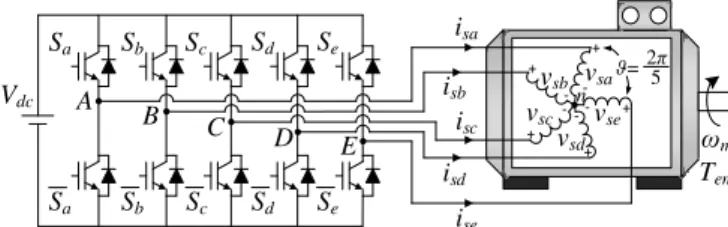
A five-phase IM with isolated neutral point and concentrated windings, driven by a five-phase two-level voltage source inverter (VSI), will be used as a case study to analyse the performance of the proposed controller. A simplified scheme of the entire system is shown in Fig. 1. The

Vdc isa + -vsb vsa + -+ vsc -vse -+ -vsd + Sb Sc Sd Se Sa n A B _C D _E Sa Sb Sc Sd Se isb isc ise isd ϑ=2π₅ ωm Tem

Fig. 1. Schematic diagram of the five-phase IM drive with

isolated neutral point and concentrated windings

controller is based on a model of the system, so this section starts with a description of the applied model. Then, the electrical limits that will be considered during the analysis are detailed.

2.1. Modelling of a five-phase IM with isolated neutral point and concentrated windings

The voltage, flux and torque equations of an electromechanical system are usually obtained considering that the iron losses and slot effects can be neglected. In this work, first and third harmonics’ components must be considered because they contribute to the generation of electrical torque [8], and the system is modelled in phase coordinates as it is shown in (1)–(4). This model includes magnetic coupling effects between phase windings, making extremely complex the design of any controller, and must be completed with the power converter (five-phase two-level VSI) equations. Then, each inverter leg is composed by two semiconductors operating in on and off states (see Fig. 1), and a finite number of possible combinations of the switching states appears. In this case, 25_{=32 switching states can be}

generated. These switching states will be represented in what follows by the vector Sn=[Sa, Sb, Sc, Sd, Se]T, being n=0,…,31. Stator phase voltages are obtained from this vector and the DC-link voltage (Vdc) as stated in (5).

d d s R tλ = ⋅ + s s s v i (1) d 0 d r R tλ = = ⋅ + r r r v i (2) λs =Lss⋅ +is Lsr⋅ir (3) λr = Lrr⋅ +ir Lrs⋅is (4) 4 1 1 1 1 1 4 1 1 1 · 1 1 4 1 1 5 1 1 1 4 1 1 1 1 1 4 a b dc c d e S S V S S S − − − −         − − − − _{ }       = − − − −     − − − −       _{− − − −}      s v (5)

The elements in equations (1)–(5) are:

• vs= [vas, vbs, vcs, vds, ves]T, is= [ias, ibs, ics, ids, ies]T, λs= [λas,

λbs, λcs, λds, λes]T and vr= [var, vbr, vcr, vdr, ver]T, ir= [iar, ibr,

icr, idr, ier]T, λr= [λar, λbr, λcr, λdr, λer]T are stator and rotor voltage, current and flux vectors in phase coordinates, respectively.

• Lss and Lrr are the stator and rotor inductances matrices,

respectively, while Lsr is the mutual inductance matrix and

3

( )

( )

( )

1 1 1 1 1 1 1 1 1 1 3 3 3 3 2 4 6 8

cos cos cos cos cos

5 5 5 5

2 4 6 8

sin sin sin sin sin

5 5 5 5

2 2 4 6

cos 3 cos 3 cos 3 cos 3

5 5 5 e e e e e e e e e e e e e e π π π π θ θ θ θ θ π π π π θ θ θ θ θ π π π θ θ θ θ         − − − −                         − −  −  −  −  −  −  −  −              =  −   −  −     T

( )

3 3 3 3 3 3 8 cos 3 5 5 2 4 6 8

sin 3 sin 3 sin 3 sin 3 sin 3

5 5 5 5 1 1 1 1 1 2 2 2 2 2 e e e e e e π θ π π π π θ θ θ θ θ              _{   }  −  _{   }         _{       } _{− −  −  −  −  −  −  −  − }                  (6)

A coordinate transformation is usually applied to

introduce two independent reference frames, called dq1 and

dq3, which contain different harmonic components. While

fundamental components are included in the dq1 subspace,

dq3 is associated with third harmonic components in the

electrical system. The coordinate transformation is well-known in the scientific literature [8], and it is based on the extended Park transformation matrix T detailed in (6), shown at the top of the page. Using (1)–(6), a new set of equations that models the five-phase IM with isolated neutral point and concentrated windings can be obtained:

1 1 1 1 1 1 3 3 3 3 3 3 1 1 1 1 3 3 3 3 0 0 0 0 0 0 0 0 0 3 0 0 3 0 sd sd sd sq sq sq s sd sd sd sq sq sq sd e sq e e sd e sq v i v i _d R v i d t v i λ λ λ λ λ ω λ ω ω λ ω λ              _{= ⋅} ₊  ₊                           −           +_{ }⋅_{ } − _{ }  _{  }     (7) 1 1 1 1 1 1 1 1 3 3 3 3 3 3 3 3 1 1 1 3 3 0 0 0 0 0 0 0 0 0 0 0 0 0 0 0 0 0 0 0 0 0 0 0 0 0 3 0 0 3 0 rd r rd rd rq r rq rq r rd rd rd r rq rq rq rd sl sl sl sl v R i v R i d R v i dt R v i λ λ λ λ λ ω ω ω ω                      ₌ ₌ _⋅ ₊  ₊                       _{   }           −       +_{ }⋅ −     1 3 3 rq rd rq λ λ λ               (8) 1 1 1 1 1 1 3 3 3 3 3 3 1 1 1 1 3 3 3 3 0 0 0 0 0 0 0 0 0 0 0 0 0 0 0 0 0 0 0 0 0 0 0 0 sd s sd sq s sq s sd sd s sq sq rd m rq m m rd m rq i L i L L i L i i L i L L i L i λ λ λ λ              ₌ _⋅ ₊               _{ }                   +_{ }⋅_{ }    _{  }     (9) 1 1 1 1 1 1 3 3 3 3 3 3 1 1 1 1 3 3 3 3 0 0 0 0 0 0 0 0 0 0 0 0 0 0 0 0 0 0 0 0 0 0 0 0 rd r rd rq r rq r rd rd r rq rq sd m sq m m sd m sq i L i L L i L i i L i L L i L i λ λ λ λ              ₌ _⋅ ₊               _{ }                   +_{ }⋅_{ }    _{  }     (10) 1 1 1 1 3 3 3 3 s ls m r lr m s ls m r lr m L L L L L L L L L L L L +         +  ₌     ₊      +     (11) 1 1 1 3 0 3 0 3 t t e e r sl e e r sl dt dt θ ω ω ω θ ω ω ω +       = =      ₊   



 



  (12) where:

• vsd1, vsq1, isd1, isq1 and vsd3, vsq3, isd3, isq3 are the projections

of the stator phase voltages and currents in the subspaces

dq1 and dq3, respectively.

• vrd1, vrq1, ird1, irq1 and vrd3, vrq3, ird3, irq3 are the projections

of the rotor phase voltages and currents in the subspaces

dq1 and dq3, respectively.

• λsd1, λsq1and λsd3, λsq3 are the stator fluxes in the subspaces

dq1 and dq3, respectively.

• λrd1, λrq1and λrd3, λrq3 are the rotor fluxes in the subspaces

dq1 and dq3, respectively.

• Lls, Llr are the stator and rotor leakage inductance, respectively.

• Lm1, Lm3 are the fundamental and third harmonic mutual

magnetic inductance between stator and rotor,

respectively.

• θe1, θe3 are the rotating electrical angles for the dq1 and dq3

subspaces, respectively.

• ωe1, ωe3 are the rotating electrical speeds for the dq1 and

dq3 subspaces, respectively, while ωsl is the slip speed and

ωr is the rotor angular speed defined as p·ωm, being p the

number of pole pairs and ωm the mechanical speed.

This model can be used to control the system, and it is characterised by constant dq1 and dq3 values in steady state.

Following this approach, the generated torque is determined by the sum of those developed in the independent frequency-domain subspaces, as it is stated down below:

1 3 em em em T =T +T (13) 1 1 1 1 1 1 em m rd sq rq sd T = pL _i i −i i _ (14) 3 3 3 3 3 3 3 em m rd sq rq sd T = pL _i i −i i _ (15)

being Tem1 and Tem3 the electromagnetic torques created by the

4

2.2. Electrical constraints for the control strategy

The imposed electrical limits will maximise the torque capability of the system without exceeding the safety values of the machine and the VSI. The voltage limit comes from the maximum DC-link voltage that the VSI can apply to the machine (maximum peak phase-to-phase voltage, Vdc). It is obtained in the flux-weakening region, where the available torque decreases when the machine operates above the base speed. On the other hand, current limits are imposed by the power converter and the electric machine. Power switches

impose a maximum peak phase current value IVSI, while the

copper losses in the machine establish a maximum RMS phase current IRMS. For the sake of simplicity, it is considered in what follows that the RMS phase current never exceeds the maximum available. Then, the electrical constraints that will be considered are summarised here:

( )

phase VSI i t ≤I (16)

( )

phase to phase dc u _{− −} t ≤V (17)

Note also that, in order to avoid the magnetic saturation in the machine, the maximum peak of the magnetic field must be limited. This paper tries to begin to consider this limitation in the control strategy but taking into account a series of starting hypotheses. In this way, a starting point is established in the study of the magnetic saturation and its inclusion in the control of multiphase machines. First, the used model for the multiphase machine is linear and does not consider any non-linearity due to the magnetic field saturation. Next, suppose that the machine is only fluxed with the first and third harmonic components, and they are synchronised. Therefore, the air-gap magnetic field H can be expressed as follows:

( )

1co s

( )

3co s 3

( )

H ϕ = H ϕ −H ϕ (18)

where H1 and H3 are the amplitudes of every harmonic

component, while the angle φ varies in the range [–π/2, π/2]. The maximum value of H must be limited to HM, which is usually selected to avoid the magnetic saturation, as shown in the following equation:

[ ]

{

1

( )

3

( )

}

/ 2 , / 2

co s co s 3 _M

m a x H H H

ϕ∈ −π π ϕ − ϕ ≤ (19)

If the effect of the leakage fluxes is neglected, this limitation can be forced in terms of the stator currents in the

d1 and d3 axes (flux-producing currents of the machine),

writing (19) in the following way (see [11] for more details):

[ ]

( )

( )

3 , 1 , / 2, / 2 cos 3 cos 3 sd M max sd sd rated i I max i I ϕ∈ −π π ϕ ϕ   =  − ≤   (20)

where Isd,rated is the rated magnetising current of the machine, i.e. the magnetising current that produces the rated sinusoidal spatial distribution of the air-gap magnetic field. This equation is a new electrical limit that must be taken into account in the control strategy. The solution of (20) yields to the expressions presented in (21) and (22), as it is explained in [11], which constitute the maximum magnetisation level considering the previous hypotheses.

1, , 2 3 s d m a x s d r a te d i = I (21) 3 , , 1 3 s d m a x s d r a te d i = I (22)

3. Definition of the proposed predictive controller

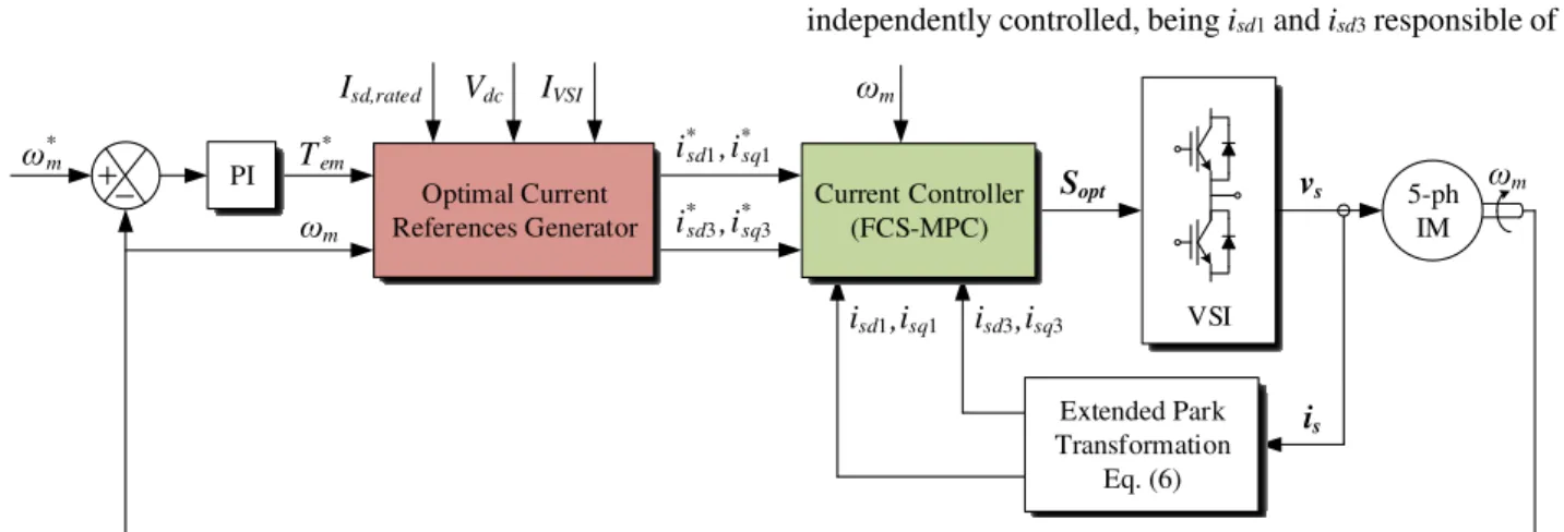
The general scheme of the proposed control strategy applied to the five-phase machine is presented in Fig. 2. It is formed by an outer speed control loop based on a conventional Indirect Rotor Field Oriented Control (IRFOC) and two MPC stages to obtain the optimal dq current reference and to implement the inner current controller. As it was mentioned in the introduction section, one interesting characteristic of the proposal is that electrical limits are easily included in the controller. A detailed description of this general scheme will be given in this section.

First, the flux and torque are decoupled for the control purpose, following the conventional IRFOC idea. In the dq reference frame, it is assumed that fundamental and third

harmonic rotor flux components are only attached to d1 and

d3 axes, respectively, while no linkages exist on the q1 and q3

axes, as stated by:

1 1 0 rq rq d d t λ = λ = (23) 3 3 0 rq rq d d t λ = λ = (24)

In this situation, torque and flux production are independently controlled, being isd1 and isd3 responsible of the

, i*sd3 i*sq3 Sopt ωm T*em Vdc Current Controller (FCS-MPC) Extended Park Transformation Eq. (6) ωm is Optimal Current References Generator ωm VSI 5-ph IM , i*sd1 i*sq1 vs PI isq1 isd1, isd3,isq3 ω*m Isd,rated IVSI

5 regulation of the two rotor fluxes (fundamental and third

harmonic), while isq1 and isq3 are related to the electrical

torque production of first and third space harmonics, respectively.

Then, a first control stage is in charge of obtaining optimal references for the dq currents using an optimisation process based in a continuous-control-set MPC technique [17]. This control stage utilises the machine model, cost functions and analytical methods to obtain the optimal references for the next control stage, where optimization methods such as quadratic programming are normally used to deal with the imposed constraints [18,19]. In this work, the objective of this optimisation stage is to get the expected torque along with the minimisation of the copper losses, while respecting the defined maximum peak values of currents, voltages and the magnetisation level. Consequently, the optimisation problem to be solved is summarised in (25), where two weighting factors σi and σT are introduced in the objective function f to give more or less importance to the minimisation of the copper losses with respect to the reference torque tracking. Note also that it is required to discretise the model of the multiphase drive and the Euler method is used for this purpose. The discretised model is utilised to obtain the predicted phase voltages and currents that are used to compute the objective function and to calculate the peak values that constraint the optimisation problem.

(

)

(

)

(

)

(

)

[ ]

( )

( )

( ) ( )

2 2 2 2 2 * 1 1 3 3 3 , 1 , / 2, / 2 : , , , , , , , cos cos 3 3 and respecting equations 7 15

i sd sq sd sq T em em max sa sb sc sd se VSI max ab ac ad ae dc sd M max sd sd rated min f i i i i T T subject to I peak i i i i i I V peak u u u u V i I max i I ϕ π π σ σ ϕ ϕ ∈ −   =_ + + + + − _   = ≤ = ≤   =  − ≤   − (25)

The selection of appropriate values for the weighting factors has been made through the following analysis. The drive has been analytically studied (a simulation environment

based on MATLAB® _{tools is used) within the valid operating}

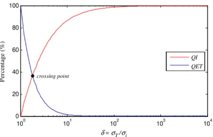
region, where the ratio δ = σT/σi has been varied while the quadratic stator current QI = isd12 + isq12 + isd32 + isq32 and the

torque quadratic error QET = (T*

em – Tem)2 terms have been evaluated. With the intention of making a fair comparison, QI and QET have been represented in a dimensionless manner, i.e. in terms of a percentage relative to their maximum values obtained in this test. Figure 3 depicts these dimensionless QI and QET values for one operating point (the reference speed is set at 20 rad/s with a torque of 6 N-m) and different δ values. The crossing point of QI and QET curves represents a trade-off between copper losses reduction and torque tracking error. For example, the crossing point in the plotted case shows a value of δ = 1.82, which corresponds to a 36.68% of copper

100 101 102 103 104 0 20 40 60 80 100 δ = σ_T /σ_i P er ce n ta g e (% ) QI QET crossing point

Fig. 3. Evaluation of QI and QET terms using different δ

values when the machine is driven at a particular operating point (20 rad/s and 6 N-m)

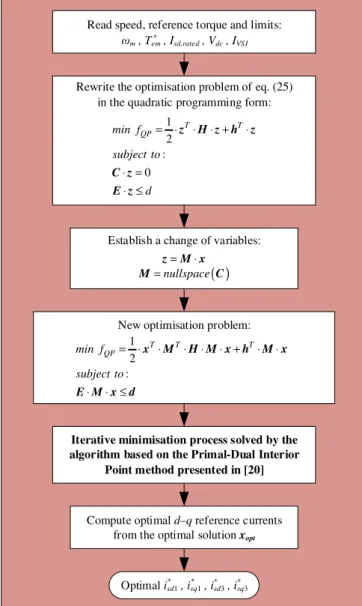
losses and the same percentage of torque tracking error (both with respect to their maximum values in the test). It is interesting to mention that quite similar plots are obtained when different operating points are considered (Table 1 summarises these results for different operating points). However, since the final objective is to control the machine at the desired speed and torque, the reduction of the torque tracking error must predominate and the δ value should be higher than the ones of the crossing points. Therefore, a value of δ>5 seems to be an appropriate choice, guaranteeing good torque tracking in the system. In this case, the weighting factors are set to σi = 1 and σT = 10 to ensure good torque tracking in the whole operating region and, when it is also possible, reduce the copper losses in the multiphase machine. On the other hand, Fig. 4 summarises the process to obtain the optimal dq reference currents, where the proposed optimisation problem in (25) is first rewritten in the standard form of a quadratic programming problem (see second block of Fig. 4). In this new quadratic programming form, z is the primal optimisation variable regrouping the states and inputs of the system’s model, H and h are the quadratic and linear parts of the objective function, respectively, while matrices C, d and E represent the dynamics constraints. Since it is very difficult to solve this problem in real time, a change of variables is proposed with the aim of reducing the complexity (see third block of Fig. 4), where x is the dual variable and M represents the null space of C, i.e. C·M=0. The minimisation problem resulting from this change of variables has less constraints and is finally solved through an iterative process based on the Primal-Dual Interior Point method for constrained nonlinear optimisation, as it is detailed in [20].

Once the optimal reference currents have been determined, the second stage of the proposed controller is applied. This second stage is an inner stator current controller based on the FCS-MPC method, which is detailed in the flow diagram shown in Fig. 5 and in the block diagram of Fig. 6. The effective implementation of the FCS-MPC method uses a second-step ahead prediction to compensate the delay in the

Table 1 A representative set of obtained QI and QET values as well as their crossing points at different working conditions Reference torque

(N-m), T* em

Mechanical speed (rad/s), ωm

20 60 100 140 180

2 36.90%, δ=1.77 36.90%, δ=1.77 36.90%, δ=1.77 26.95%, δ=3.29 34.68%, δ=2.35 4 36.72%, δ=1.81 36.73%, δ=1.81 34.53%, δ=2.28 37.05%, δ=1.77 37.91%, δ=1.69 6 36.68%, δ=1.82 36.65%, δ=1.82 37.66%, δ=1.66 34.96%, δ=1.60 38.87%, δ=1.72 8 36.66%, δ=1.83 41.62%, δ=1.21 37.42%, δ=1.75 36.57%, δ=1.72 38.29%, δ=1.51

6

Establish a change of variables:

New optimisation problem:

Optimal isd*1 , isq*1 , isd*3 , isq*3

Iterative minimisation process solved by the algorithm based on the Primal-Dual Interior

Point method presented in [20]

Rewrite the optimisation problem of eq. (25) in the quadratic programming form: Read speed, reference torque and limits:

ωm , Tem* , Isd,rated , Vdc , IVS I

Compute optimal d–q reference currents from the optimal solution xopt

( ) nullspace = ⋅ =z M x M C 1 2 : 0 T T QP min f subject to d = ⋅ ⋅ ⋅ + ⋅ ⋅ = ⋅ ≤ z H z h z C z E z 1 2 : T T T QP min f subject to = ⋅ ⋅ ⋅ ⋅ ⋅ + ⋅ ⋅ ⋅ ⋅ ≤ x M H M x h M x E M x d

Fig. 4. Flow diagram for the optimisation process for the

reference current generation

computation of the control signals, which it is comparable with the sampling time (see [14] for details). Consequently, the discretised model is applied in the sampling period k to estimate the stator current values in k+2, isdqk+2, using the

measured mechanical speed and stator currents, ωmk and isdqk

respectively. Once the prediction is done, the controller determines the applied stator voltage or switch configuration of the multiphase VSI (Soptk+1) in order to minimise the

predefined cost function J, see (26). This cost function represents the control objective of the FCS-MPC method, being in this case the tracking of the optimal current references calculated by the optimisation algorithm, although different cost functions can be used to include other control constraints and depending on the specific application. For instance, a different cost function in order to reduce the VSI losses or the stator current harmonic content is proposed in [21], where weighting factors are also introduced to weight the control action between current tracking and losses reduction. Finally, the switching state Soptk+1 is obtained

through an exhaustive search process, where the predictive

model is computed for every available switching state (25₌₃₂

for a five-phase machine) to find the future stator current that minimises J.

Initiate the cost function:

J0←∞ , n←1 Take Snk+1 If J < J0 Jo←J Soptk+1←Snk+1 n=n+1 NO YES Instant k k−1 k+1 If n < 32 YES Apply Soptk+1 NO Read future current reference:

, , , i* k+2

sd1 i* k+sq1 2 isd* k+3 2 i* k+sq3 2

i* k+2 ₌ sdq

Produce a prediction of stator current at time k+2:

isd1k+2 , isq1k+2 , isd3k+2 , isq3k+2

i k+2

=

sdq

Read current and speed for sample k:

isd1k , isq1k , isd3k , isq3k , ωmk i k sdq =

Produce a prediction of stator current at time k+1:

isd1k+1 , isq1k+1 , isd3k+1 , isq3k+1

i k+1 ₌ sdq

Evaluate J using eq. (26)

Fig. 5. Flow diagram of the switching state selection during

a certain period using the FCS-MPC technique

J abcde dq Table of possible voltage vectors PREDICTIVE MODEL Minimizer min(J) Cost function computation Eq. (26) FCS-MPC ωm k Sopt Sn i* k+2 sdq i k sdq i k+2sdq i k s

Fig. 6. Block diagram for the second control stage based on

7

(

) (

)

(

) (

)

2 2 * 2 2 * 2 2 1 1 1 1 2 2 * 2 2 * 2 2 3 3 3 3 k k k k sd sd sq sq k k k k sd sd sq sq J i i i i i i i i + + + + + + + + = − + − + + − + − (26)

Note that future values for the reference currents are needed in the cost function. In this sense, the optimal reference values are usually assumed to be constant in the dq reference frame for sufficiently small sampling times (see [21]):

* k 2 * k 1 * k

sd q sd q sd q

i + ≈i + ≈i (27)

4. Validation of the proposed method

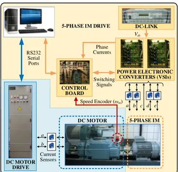
In this section, experimental results are presented in order to validate the feasibility of the proposal. This is done using the experimental test rig presented in Fig. 7, which is principally composed by a three-phase IM rewound to have five phases with 30 slots and three pairs of poles. The electrical parameters and considered electrical limits are gathered in Table 2. The machine is supplied by two three-phase inverters from SEMIKRON, connected to a DC- link voltage of 300 V from an independent DC power supply. The control algorithm is implemented in a TM320F28335 DSP placed on a MSK28335 Technosoft board. An external programmable load torque is also introduced in the system by means of an independently controlled DC motor. Finally, the

rotor mechanical speed is measured using a

GHM510296R/2500 encoder that is coupled to the shaft of the multiphase IM, while the torque is estimated based on the measured currents.

Note that the computational power capacity of our control system is not enough to solve the optimisation problem online. Then, the optimal dq reference currents were obtained offline, applying the optimisation stage in a previous step and storing the obtained values in look-up tables. The reference torque and speed are consequently used during the normal operation of the drive to access these look-up tables and get the reference values for the inner online current controller. Under these conditions, the computational requirement of the control algorithm is about 35 µs, which permits the use of a sampling frequency of 15 kHz (the sampling period is 67 µs).

The present study starts by analysing the ability of the reference current generator to produce optimal dq references in all the speed range that produce the maximum torque while respecting the imposed limits and minimising the copper losses. Five experimental tests have been conducted to study the steady-state performance of the system when the optimised references are applied in the available speed range. All the experiments have been carried out applying a constant reference speed of 20, 40, 60, 80 and 100 rad/s, and a load torque equal to the maximum available one to reach the electrical limits and force the optimisation block action. The machine is driven to the steady state and the obtained results are shown in Fig. 8, where the mean values of the electrical torque and reference stator currents are plotted with filled circles. The maximum values of phase-to-phase stator voltages and phase stator currents (normalised to their limit values, Vdc and IVSI, respectively) are shown in Fig. 8, where two regions can be clearly identified. The third harmonic is fully exploited to produce the maximum torque while

Current Sensors DC MOTOR 5-PHASE IM a b DC MOTOR DRIVE RS232 Serial Ports 5-PHASE IM DRIVE Switching Signals Phase Currents CONTROL BOARD Speed Encoder (ωm) DC-LINK Vdc a b c d e POWER ELECTRONIC CONVERTERS (VSIs)

Fig. 7. Graphic diagram of the experimental system

Table 2 Machine parameters and electrical limits

Parameter Value

Stator resistance Rs 19.45 Ω

Rotor resistances Rr1 and Rr3 13.54 Ω

Stator leakage inductance Lls 100.7 mH

Rotor leakage inductance Llr 38.6 mH

Mutual inductance Lm1 656.5 mH

Mutual inductance Lm3 72.9 mH

Pole pairs p 3

Voltage limit Vdc 300 V

Current limit IVSI 2.5 A

Rated d-current Isd,rated 0.9 A

Maximum torque Tem,max 8.13 N-m

respecting the current limit in region 1, named constant torque region. The voltage limit is never reached and the flux-components of the current, isd1 and isd3, do not exceed their

maximum values of equations (21) and (22), respecting the maximum magnetisation level. Region 2, or torque breakdown region, starts when the DC-link voltage becomes insufficient to inject the maximum phase current. When the voltage limit is reached, the flux-weakening is forced in the drive and the generated electrical torque is gradually reduced with the speed. Since the third harmonic component of the magnetic field requires an important portion of the DC-link voltage in detriment of the fundamental component, and this last component mostly generates the electrical torque in the machine, the reduction in dq3 currents is larger than in dq1

currents in region 2, being nearly zero at high speed.

An important issue in concentrated winding electrical drives is the torque enhancement due to the third harmonic injection. A comparison of the maximum obtained torque with and without third harmonic injection is detailed in Fig. 9, where previous experiments were reproduced forcing zero

isd3 and isq3 reference values. Again, filled circles represent the

obtained experimental results, and a significant increment in the obtained maximum torque can be observed (about 26% in

region 1). It is important to remark that a MATLAB®

8 simulate the system and obtain the plotted curves in order to

complete the results of the experimental analysis (filled circles), avoiding the record and memory limitations of the control board and reducing the number of experiments in the considered speed range.

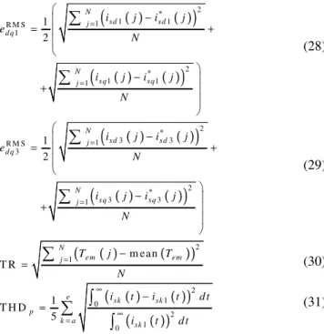
Tables 3 and 4 summarize the quantitative analysis of the experimental results presented in Fig. 9, where cases with and without injection of third harmonic are respectively considered in steady state. The analysis is made on the basis of: i) the root-mean-squared (RMS) error in the current tracking for each dq subspace (edqRMS1 and edqRMS3 ), ii) the torque

ripple (TR), and iii) the total harmonic distortion in the phase

currents (THDp), where the figures of merit are computed as

follows:

( )

( )

(

)

( )

( )

(

)

2 * 1 1 1 R M S 1 2 * 1 1 1 1 2 N sd sd j d q N sq sq j i j i j e N i j i j N = =  −  =  +    −  +   





(28)

( )

( )

(

)

( )

( )

(

)

2 * 3 3 1 R M S 3 2 * 3 3 1 1 2 N sd sd j d q N sq sq j i j i j e N i j i j N = =  −  =  +    −  +   





(29)

( )

(

)

(

)

2 1 m ean T R N em em j T j T N = − =



(30)

( )

( )

(

)

( )

(

)

2 1 0 2 1 0 1 T H D 5 e _{sk sk} p k a _sk i t i t d t i t d t ∞ ∞ = − =







(31)

being isk1 the fundamental component of the considered

current. Notice that the THDp value is an average of all the

obtained THD stator phase currents’ values.

Note that the obtained RMS current errors and torque ripples are similar in both cases (with and without third harmonic injection). However, this is not the case when the figure of merit THDp is considered, where the injection of third harmonic components notably increases the value, being this an expected consequence of the modified control action with third harmonic injection, as it is also observed in Fig. 9. The five-phase machine with a concentrated winding topology can then use, as expected (see [9]), the first and third stator current and spatial stator flux to generate electrical torque.

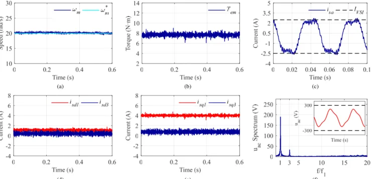
The previous analysis is complemented with some experimental tests to study the time performance of the controlled system. The first one is summarised in Fig. 10, where the maximum load torque is applied at a reference speed of 20 rad/s, being the system in steady state within the constant torque region (region 1). It can be observed a good tracking performance of the mechanical speed (Fig. 10a), while the values of the torque and dq1 and dq3 currents

correspond to optimal values previously obtained (Figs. 10b, 10d and 10e respectively). Notice that the current limit is reached in the analysed case, as it is shown in Fig. 10c, where

Region 1 Region 2

Fig. 8. Steady state analysis of the proposed controller. From

top to bottom: maximum obtained torque; d1 and d3 stator

currents; q1 and q3 stator currents; and maximum

phase-to-phase stator voltage and phase-to-phase stator current (normalised to their limit values, Vdc and IVSI, respectively)

Fig. 9. Maximum electrical torque in the experimental system

with and without the injection of third harmonic stator current components

Table 3 Quantitative analysis of the experimental results of

Fig. 9 for the cases with injection of third harmonic

Speed (rad/s) edq1 RMS (A) edq3 RMS (A) TR (N-m) THDp (%) 20 0.1808 0.2703 0.3172 23.4888 40 0.1964 0.2185 0.3154 22.7031 60 0.1988 0.2023 0.3088 22.3482 80 0.1883 0.1978 0.2825 22.0215 100 0.1909 0.1981 0.2305 21.7540

Table 4 Quantitative analysis of the experimental results of

Fig. 9 for the cases without injection of third harmonic

Speed (rad/s) edq1RMS (A) edq3 RMS (A) TR (N-m) THDp (%) 20 0.1843 0.2805 0.2919 11.2831 40 0.1888 0.2384 0.2739 9.8229 60 0.1835 0.2122 0.2492 10.7402 80 0.1752 0.2091 0.2167 13.1938 100 0.1909 0.1996 0.1882 14.0389

9 the phase current ‘a’ is plotted. The rest of the stator currents

in the multiphase machine have a similar behaviour and they are omitted in the representation for the sake of clarity. The frequency decomposition of phase-to-phase voltages is depicted in Fig. 10f, where voltage uac is shown. Interestingly enough, two peaks appear corresponding with the fundamental and third harmonic components, showing that the voltage limit is not reached during the experiment.

A second experiment is presented in Fig. 11 where the torque breakdown region is considered. The machine is

driven with a reference speed of 60 rad/s while the maximum allowable load torque at this speed is applied (about 6.4 N-m, see Fig. 11b). Under these conditions, the system is working with the optimal dq1 and dq3 stator current values obtained

from the optimisation stage (Figs. 11d and 11e), being the phase current value below the imposed limit (Fig. 11c, where only one stator phase current is again plotted for the sake of clarity, having a similar performance the rest of the stator currents). However, the voltage limit condition is reached, as it can be seen in Fig. 11f.

(a) (b) (c)

(d) (e) (f)

Fig. 10. Performance of the controlled system when the maximum load torque is applied at a reference speed of 20 rad/s. (a)

Measured mechanical speed versus the applied reference, (b) obtained electrical torque, (c) stator phase current ‘a’, (d) d1 and

d3 stator currents components, (e) q1 and q3 stator currents components, (f) time-domain performance and frequency spectrum

of the phase-to-phase voltage uac

(a) (b) (c)

(d) (e) (f)

Fig. 11. Performance of the controlled system for a reference speed of 60 rad/s and a load torque equal to the maximum available

one. (a) Measured mechanical speed versus the applied reference, (b) obtained electrical torque, (c) stator phase current ‘a’, (d) d1 and d3 stator currents components, (e) q1 and q3 stator currents components, (f) time-domain performance and frequency

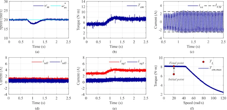
10 The dynamic operation of the controlled system has

also been studied in Figs. 12 and 13. First, a torque step test is presented in Fig. 12, where a reference speed of 20 rad/s is

imposed and a load torque (TL) step from 6.4 m to 8.13

N-m is applied. Notice that the starting systeN-m conditions N-meet both current and voltage limits, ending with a maximum torque condition where the current limit is reached within the constant torque region, as it can be appreciated in Fig. 12c. A

graphic representation of the operating point evolution is shown in Fig. 12f. From Figs. 12a and 12b it can be stated that the speed tracking performance is smooth and adequate, although a slight decrement in the value can be appreciated when the torque step is applied (the speed drops at about 18 rad/s but it is recovered after 0.7 s). Moreover, dq1 and dq3

currents (Figs. 12d and 12e) reach their optimal values, while

q-current components increase with the torque.

Initial point Final point

(a) (b) (c)

(d) (e) (f)

Fig. 12. Dynamic performance of the controlled system for a reference speed of 20 rad/s and a load torque step from 6.4 N-m

to 8.13 N-m. (a) Measured mechanical speed versus reference speed, (b) obtained electrical torque, (c) stator phase current ‘a’, (d) d1 and d3 stator currents components, (e) q1 and q3 stator currents components, (f) system evolution in the maximum

torque-speed curve

Initial point

Final point

(a) (b) (c)

(d) (e) (f)

Fig. 13. Dynamic performance of the controlled system for a speed step from 40 to 60 rad/s and a load torque equal to 6.4 N-m

(the maximum available). (a) Measured mechanical speed versus reference speed, (b) obtained electrical torque, (c) stator phase current ‘a’, (d) d1 and d3 stator currents components, (e) q1 and q3 stator currents components, (f) system evolution in the

11 Finally, a second dynamic test is obtained considering

a speed step from 40 to 60 rad/s at a load torque of 6.4 N-m (the maximum available one when the system is operated at 60 rad/s), where the system enters in the torque breakdown region. The obtained results are presented in Fig. 13, where a schematic representation of the system evolution is plotted in Fig. 13f for a better understanding of the experiment. The speed tracking is depicted in Fig. 13a, showing a settling time of about 0.8 s. The starting point of the experiment is below the electrical limits of the system. However, the voltage limit is reached when the speed step is applied in order to track the new reference speed as soon as possible. It can be appreciated that the stator current limit is also reached while the imposed reference speed step is tracked (see Fig. 13c), and dq1 and dq3

stator current components are regulated to their optimal values in Figs. 13d and 13e, respectively.

All in one, the proposed controller, based in model-based predictive control techniques, generates optimal reference currents taking into account the imposed voltage and current limits of the machine, as well as its maximum magnetisation level, showing a good regulation of the electrical machine in steady and transient states.

5. Conclusion

This paper introduces a current controller using model-based predictive control techniques that allows the optimal utilisation of the system’s torque capability under voltage, current and magnetic limitations. First, a predictive stage produces optimal current references, taking into account programmed electrical and magnetic restrictions. Then a predictive controller regulates the stator currents of the system in order to track the optimal references. The interest of the proposed controller has been verified using one of the hottest electrical machine topologies as a case example due to its promising industry perspective, such as the five-phase induction machine with concentrated windings. The obtained results prove that the optimal current references generator produces the best combination of the dq current references to obtain the maximum torque while minimising copper losses and respecting the imposed electrical limits, while an important enhancement in the torque production is achieved when the third harmonic component of the current is exploited. The dynamic operation of the system has been also tested, showing fast and smooth current and speed tracking performances. Although a particular multiphase drive and voltage, current and magnetic limitations have been considered, the proposal can be easily extended to n-phase multiphase machines, considering more complex cost functions and optimisation problems.

6. Acknowledgments

The authors would like to acknowledge the doctoral school of ENSAM, the University of Seville under VPPI-US program and the Ministerio de Economía y Competitividad of the Spanish Government under reference DPI2016-76144-R for the financial support of this work.

7. References

[1] Lemmens, J., Vanassche, P., Driesen, J.: 'Optimal Control of Traction Motor Drives Under Electrothermal Constraints', IEEE Journal of Emerging and Selected Topics in Power Electronics, 2014, 2, (2), pp. 249–263.

[2] Xu, X., Novotny, D.W.: 'Selection of the flux reference for induction machine drives in the field weakening region', IEEE Trans. Ind. Appl., 1992, 28, (6), pp. 1353–1358. [3] Harnefors, L., Pietilainen, K., Gertmar, L.: 'Torque-maximizing field-weakening control: design, analysis, and parameter selection', IEEE Trans. Ind. Electron., 2001, 48, (1), pp. 161–168.

[4] Kim, J.M., Sul, S.K.: 'Speed control of interior permanent magnet synchronous motor drive for the flux weakening operation', IEEE Trans. Ind. Appl., 1997, 33, (1), pp. 43–48. [5] Cai, X., Zhang, Z., Wang, J., Kennel, R.: 'Optimal Control Solutions for PMSM Drives: A Comparison Study With Experimental Assessments', IEEE Journal of Emerging and Selected Topics in Power Electronics, 2018, 6, (1), pp. 352– 362.

[6] Barrero, F., Duran, M.: 'Recent advances in the design, modeling and control of multiphase machines – Part 1', IEEE Trans. Ind. Electron., 2016, 63, (1), pp. 449–458.

[7] Duran, M., Barrero, F.: 'Recent advances in the design, modeling and control of multiphase machines – Part 2', IEEE Trans. Ind. Electron., 2016, 63, (1), pp. 459–468.

[8] Durán, M.J., Levi, E., Barrero, F.: 'Multiphase Electric Drives: Introduction', Wiley Encyclopedia of Electrical and Electronics Engineering, 2017.

[9] Toliyat, H.A., Lipo, T.A., White, J.C.: 'Analysis of a concentrated winding induction machine for adjustable speed drive applications. I. Motor analysis', IEEE Trans. Energy Convers., 1991, 6, (4), pp. 679–683.

[10] Levi, E., Dujic, D., Jones, M., Grandi, G.: 'Analytical determination of DC-bus utilization limits in multiphase VSI supplied AC drives', IEEE Trans. Energy Convers., 2008, 23, (2), pp. 433–443.

[11] Mengoni, M., Zarri, L., Tani, A., Parsa, L., Serra, G., Casadei, D.: 'High-torque-density control of multiphase induction motor drives operating over a wide speed range', IEEE Trans. Ind. Electron., 2015, 62, (2), pp. 814–825. [12] Kouro, S., Perez, M.A., Rodriguez, J., Llor, A.M., Young, H.A.: 'Model predictive control: MPC’s role in the evolution of power electronics', IEEE Ind. Electron. Mag., 2015, 9, (4), pp. 8–21.

[13] Lim, C.S., Rahim, N.A., Hew, W.P., Levi, E.: 'Model predictive control of a two-motor drive with five-leg-inverter supply', IEEE Trans. Ind. Electron., 2013, 60, (1), pp. 54–65. [14] Arahal, M.R., Barrero, F., Toral, S., Duran, M.J., Gregor, R.: 'Multiphase current control using finite-state model-predictive control', Control Eng. Pract., 2009, 17, (5), pp. 579–587.

12 [15] Rodriguez, J., Kazmierkowski, M.P., Espinoza, J.R.,

Zanchetta, P., Abu-Rub, H., Young, H.A., Rojas, C.A.: 'State of the art of finite control set model predictive control in power electronics', IEEE Trans. Ind. Informat., 2013, 9, (2), pp. 1003–1016.

[16] Kestelyn, X., Gomozov, O., Buire, J., Colas, F., Nguyen, N.K., Semail, E.: 'Investigation on model predictive control of a five-phase permanent magnet synchronous machine under voltage and current limits', IEEE International Conference on Industrial Technology, Seville, Spain, 2015, pp. 2281–2287.

[17] Rodriguez, J., Cortes, P.: 'Predictive control of power converters and electrical drives', John Wiley & Sons, Ltd, 2012.

[18] Ahmed, A.A., Koh, B.K., Lee, Y.I.: 'A Comparison of

Finite Control Set and Continuous Control Set Predictive Control Schemes for Speed Control of Induction Motors', IEEE Trans. Ind. Informat., 2018, 14, (4), pp. 1334–1346.

[19] Wang, Z., Zheng, Z., Li, Y., Fan, B., Li, G.: 'Predictive

current control for induction motor using online optimization algorithm with constraints', 2017 IEEE Energy Conversion Congress and Exposition (ECCE), Cincinnati, OH, 2017, pp. 4720–4725.

[20] Gomozov, O., Trovao, J.P., Kestelyn, X., Dubois, M.: 'Adaptive energy management system based on a real-time model predictive control with non-uniform sampling time for multiple energy storage electric vehicle', IEEE Trans. Veh. Technol., 2017, 66, (7), pp. 5520–5530.

[21] Kouro, S., Cortes, P., Vargas, R., Ammann, U., Rodriguez, J.: 'Model predictive control – a simple and powerful method to control power converters', IEEE Trans. Ind. Electron., 2009, 56, (6), pp. 1826–1838.