Science Arts & Métiers (SAM)
is an open access repository that collects the work of Arts et Métiers Institute of Technology researchers and makes it freely available over the web where possible.
This is an author-deposited version published in: https://sam.ensam.eu
Handle ID: .http://hdl.handle.net/10985/17520
To cite this version :
Fessal KPEKY, Farid ABED-MERAIM, El Mostafa DAYA, Ouro-Djobo SAMAH - Modeling of hybrid vibration control for multilayer structures using solid– shell finite elements - Mechanics of Advanced Materials and Structures - Vol. 25, n°12, p.1033-1046 - 2018
Modeling of hybrid vibration control for multilayer structures using solid–
shell finite elements
Fessal Kpeky1,3, Farid Abed-Meraim2,3,*, El Mostafa Daya1,3 and Ouro-Djobo Samah4
1
LEM3, UMR CNRS 7239, Université de Lorraine, Ile du Saulcy Metz Cedex 01, France
2
LEM3, UMR CNRS 7239, Arts et Métiers ParisTech, 4 rue A. Fresnel, 57078 Metz Cedex 03, France
3
Laboratory of Excellence on Design of Alloy Metals for low-mAss Structures (DAMAS), France
4
École Nationale Supérieure d’Ingénieurs, Université de Lomé, BP. 1515, Lomé, Togo
Abstract. A self-control method of vibrations is presented in this paper. This method combines the passive damping capabilities afforded by viscoelastic materials with the active control properties associated with piezoelectric materials. Active control is introduced, using the piezoelectric properties, in order to improve the reduction in vibration amplitudes that can be obtained by viscoelastic passive damping alone. To this end, a filter has been mounted between the sensors and actuators. The resulting nonlinear problem is discretized using the recently developed solid–shell finite element SHB20E, due to the advantages it offers in terms of accuracy and efficiency, as compared to standard finite elements with the same geometry and kinematics. In order to solve the discretized problem, a resolution method using DIAMANT approach is developed. A set of selective and representative numerical tests are performed on multilayer plates to demonstrate the interest of the proposed damping model. Keywords: Vibration analysis, Active-passive control, Finite elements, Solid–shell, Piezoelectric effect, Multilayer structures.
1. Introduction
The design of effective damping systems is a challenging task that engineers are stepping up with the increasing demand for structures stressed and alleviated. For this purpose, the best-known strategy, and especially the most adopted associated system, consists in incorporating viscoelastic materials with various forms. Such viscoelastic materials can be found in the form of uniform layers inserted between two elastic layers (viscoelastic core sandwiches) [1-4], or as honeycomb filled with viscoelastic materials [5-7]. Several works have been contributed in this field, such as Akoussan et al. [8], who proposed a sensitivity analysis with regard to different parameters for sandwich plates using the Asymptotic
Numerical Method (ANM) combined with the Automatic Differentiation [9]. Worth mentioning are also the major contributions of Ferreira et al. [4] as well as Filippi et al. [10], who used Carrera’s Unified Formulation (CUF) [11-13] for the analysis of sandwich laminated plates.
Alternatively, core material systems can be found in entangled fibers [14, 15], or as viscoelastic inclusions embedded in elastic layers [16]. Unfortunately, this technique does not always allow effective passive damping. To improve the damping properties, it is sometimes necessary to increase the thickness of the viscoelastic layer. However, limitations are quickly encountered in terms of dimensions and mechanical properties of composites, which become less resistant as the thickness of the viscoelastic layers becomes larger. Other limitations are sometimes associated with the total thickness of the structure, which is related to its practical implementation. To overcome these restrictions while increasing the damping properties of multilayer structures, the use of piezoelectric materials is desirable and sometimes even unavoidable. Indeed, the attractive properties of piezoelectric materials, and especially their ability to deform under electrical load and vice versa, make them indispensable. More specifically, the current generated by deformation is collected and amplified or attenuated in order to control the vibration amplitudes. Some literature studies effectively combined passive damping and active control using viscoelastic core sandwiches constrained by layers of piezoelectric materials [17, 18]. Controlling this phenomenon is therefore important to better implement these hybrid control systems. In the literature, a number of works have been devoted to this issue, among which the contributions reported in references [19, 20]. In particular, it is clearly shown in these works that the finite element discretization leads to frequency-dependent nonlinear problems. The complexity of such problems restricted the earlier investigations to PD (Proportional Derivative) type of control laws (see Duigou-Kersulec [19] and Boudaoud [20], among others).
In this paper, we propose a method that combines the solid–shell finite element concept [21-24] and the DIAMANT approach [25-27] to effectively solve vibration problems. Accordingly, the discretization of the resulting vibration problem is achieved using the quadratic piezoelectric solid–shell finite element SHB20E developed in [28, 29]. The latter represents the extension to piezoelectric materials of the solid–shell element SHB20 proposed by Abed-Meraim et al. [30], which shows a number of advantages and capabilities compared to its counterpart, the traditional twenty-node finite element resulting from a standard displacement-based formulation. With regard to the DIAMANT approach, the latter consists of a recently developed method that combines the Automatic Differentiation with the Asymptotic Numerical Method. This technique has been proposed in [25-27], where it has been used to effectively solve problems of passive vibration damping for viscoelastic core sandwiches. Compared to these earlier contributions, the current work represents an extension that is specifically intended to solve problems of active-passive vibration damping.
2. Formulation and discretization of the problem of active-passive vibration control In this section, we consider the vibration problem of multilayer structures combining elastic, viscoelastic and piezoelectric layers. The contribution to damping of the viscoelastic material results in frequency dependency of the viscoelastic modulus E( )
ω
. Regarding the piezoelectric material, the latter induces electromechanical coupling. Therefore, we will first recall some characteristic features associated with this coupling. Then, the finite element discretization of the problem of vibrations of multilayer structures combining these materials will be carried out.2.1. Electromechanical constitutive equations
Piezoelectric materials have the capability of generating electricity when subjected to mechanical loading (sensors). Conversely, they also have the ability to deform under electrical charging (actuators). These properties are described by the following coupled electromechanical equations: T = ⋅ − ⋅ = ⋅ + ⋅ C e e
σ
ε
σ
ε
σ
ε
σ
ε
εεεε
E D κκκκ E (1)where σ and ε represent, respectively, the vector form of the stress and strain tensors; D and E denote the electric displacement and electric field vector, respectively; while C, e and
κ
stand for the elastic, piezoelectric and dielectric permittivity matrix, respectively.The discretized forms
{ }
ε and{ }
E for the strain tensor and the electric field vector are related, respectively, to the discretized displacement{ }
u and to the discretized electric potential{ }
φφφφ , using the discrete gradient operators
B
u
and
B
φ
, as follows:{ }
{ }
{ }
{ }
u φ = = − B B ε u E φφφφ (2)In the current contribution, the discrete gradient operators
B
u
and
B
φ
are obtained by finite element discretization for both the recently developed piezoelectric solid–shell formulation SHB20E (see Fig. 1), and its counterpart, the standard twenty-node piezoelectric solid element HEX20E.2.2. Discretization of the problem
The variational principle pertaining to piezoelectric materials, which provides the governing equations for the associated boundary value problem, is described by the Hamilton principle [31]. In this weak form of equations of motion, the Lagrangian and the virtual work
are appropriately adapted to include the electrical contributions, in addition to the more classical mechanical fields
v s p V V V S v s p V V S dv dv dv ds dv dv ds ρ δ δ δ δ δ δ δ δ δ − ⋅ − ⋅ + ⋅ + ⋅ + ⋅ = − ⋅ + ⋅ + ⋅ + ⋅
∫
∫
∫
∫
∫
∫
∫
ɺɺ σ εσ εσ εσ ε φ φ φ φ φ φ φ φ φ φ φ φ u u f u f u f u D E q q q (3)where
ρ
is the material density; qv, qs and q denote volume, surface and point charge, p respectively; while fv, fs and f represent volume, surface and point force, respectively. pThe finite element discretization of the boundary value problem governed by Eq. (3) generally leads to the following system of discretized equations:
{ }
{ }
{ } { }
{ }
{ } { }
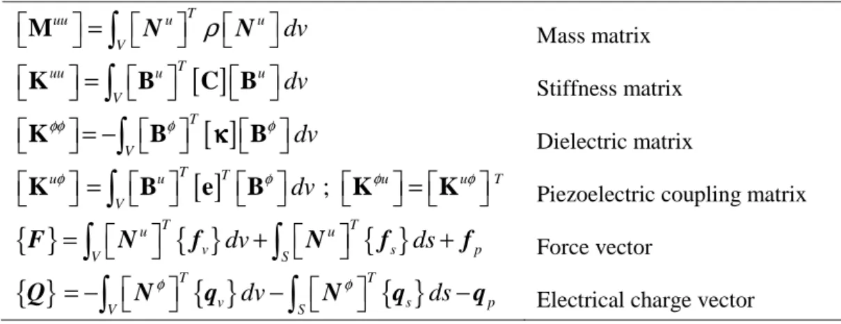
( ) uu uu u u φ φ φφ ω + + = + = M K K K K ɺɺ U U F U Q φφφφ φφφφ (4)where all matrices and vectors involved in Eq. (4) are explicitly defined in Table 1.
The above matrices are obtained by finite element discretization using both the recently developed piezoelectric solid–shell element SHB20E and the standard twenty-node piezoelectric solid element HEX20E. The formulation of the SHB20E solid–shell element is only briefly outlined hereafter; the interested reader may refer to [29] for the complete details. 2.3. Solid–shell finite element formulation
2.3.1. Kinematics and interpolation
The above-described vibration problem is discretized here using the piezoelectric solid– shell element SHB20E. The latter is an extension of the quadratic solid–shell element SHB20, which has been originally proposed by Abed-Meraim et al. [30]. The starting point for this piezoelectric extension is the addition of one piezoelectric degree of freedom (DOF) to each node. The resulting SHB20E element denotes a twenty-node hexahedral element. Based on a fully three-dimensional approach, this element has three displacement DOFs as well as one piezoelectric DOF per node. Nevertheless, to improve the performance of this solid–shell element, and to provide it with some desirable shell features, a number of enhancements are introduced within its formulation based on the assumed-strain method (ASM). In particular, a special direction is chosen, designated as the “thickness”, normal to the mean plane of this element, along which a user-defined number of integration points are arranged. Also, an in-plane reduced-integration rule is used, with 4 n× int integration points (see, e.g., Fig. 1, in the particular case when the number of through-thickness integration points is nint=3).
For this element, the spatial coordinates xi are related to the nodal coordinates xiI using the conventional quadratic shape functions, as follows:
(
, ,)
i iI Ix = x N ξ η ζ (5)
where i represents the spatial directions and ranges from 1 to 3; while I stands for the node number, which ranges from 1 to 20. Likewise, the displacement field ui is related to the nodal displacements uiI using the same quadratic shape functions, and the same applies to the electric potential
φ
in terms of its nodal values φI :(
)
(
)
, , , , u i iI I I I u u N Nφ ξ η ζ φ φ ξ η ζ = = (6)Note that in Eqs. (5) and (6) above, the convention of implied summation over the repeated index I has been adopted.
2.3.2. Discrete gradient operators
The discrete gradient operators
B
u and
B
φ
, which are associated with the above finite element discretization (see Eq. (2)), can be derived in the following compact form:1 ,1 2 ,2 1 ,1 3 ,3 2 ,2 2 ,2 1 ,1 3 ,3 1 ,1 3 ,3 3 ,3 2 ,2 ; T T T T T T T T u T T T T T T T T T T T T T T T T h h h h h h h h h h h h α α α α α α φ α α α α α α α α α α α α α α α α α α + + + + = + + = + + + + + + 0 0 0 0 0 0 B B 0 0 0 b γ b γ b γ b γ b γ b γ b γ b γ b γ b γ b γ b γ (7) where T i b , hα,i and T α
γ have been fully detailed in [30]. Note again that, in Eq. (7) and in what follows, the convention of implied summation over the repeated index α is adopted, with α ranging from 1 to 16.
The discrete gradient operators given by Eq. (7) allow us to compute the stiffness matrix uu
K , the piezoelectric matrix K and the dielectric matrix uφ K . In the same way, the φφ corresponding mass matrix M , involved in the vibration problem governed by Eq. (4), is uu easily computed using the classical shape functions associated with these quadratic elements. Once the governing equations have been discretized in the form of Eq. (4), it is relevant to develop an effective method for solving the associated nonlinear problem, which will be the object of the next section.
3. Methods and laws for active vibration control
Several methods have been proposed for the control of vibrations using piezoelectric materials. Some of these strategies are based on the optimum position of the piezoelectric
patches [32-34]. Other techniques, such as the LQR (Linear Quadratic Regulator) [35-37] and the LQG (Linear Quadratic Gaussian) [38, 39], for instance, determine the gain control for the best control of vibrations. We will limit ourselves in this work to the use of retroactive control laws, which connect the electrical potential at the edges of the actuators to the one at the edges of the sensors. Hence, this allows the use of more complex and elaborate control laws, such as a filter of transfer plugged between the actuators and sensors.
3.1. Proportional Feedback Control
In this type of control, the voltage generated in the layer set as sensor is amplified and fed back via a controller in the other layer used as actuator. In fact, when a structure vibrates, the deflection of the piezoelectric layers results in electric potential generation. Hence, by denoting the voltage generated at the sensor and at the actuator as
φφφφ
s andφφφφ
a, respectively, the control can be expressed in a comprehensive manner in the form{ }
φφφφa =H( )ω{ }
φφφφs (8)where H( )
ω
represents the transfer function of a filter in the circuit connecting the sensor to the actuator, as illustrated in Fig. 2. By separating the different layers of the structure and by applying only a harmonic force F =F0ei tω to the system, one can rewrite Eq. (4), which describes the vibration of a structure, in the form2 ( ) 0 0 0 0 0 0 0 0 0 0 0 0 s a s s a a u u uu uu u s u a φ φ φ φφ φ φφ ω ω K K K M K K K K U F φφφφ φφφφ − = (9)
The voltage generated at the sensor can therefore be written as
{ }
s 1 us{ }
s φφ φ K − K = − Uφφφφ
(10)Combining Eq. (10) with Eq. (8), one obtains
{ }
( ) s 1 us{ }
a H φφ φω
K − K = − Uφφφφ
(11)Substituting Eqs. (10) and (11) in the first line of Eq. (9), and expressing the stiffness matrix as Kuu( )ω =Kuu0+E( )ω Kuuv, one can get
{ } { }
2 0E
( )
ω
vH
( )
ω
pω
K
K
K
M
+
−
−
=
U
F
(12)0 0 1 1 with a s s s s s uu sensor u u uu actuator v v u u p actuator sensor uu φ φφ φ φ φφ φ K K K K K K K K K K K K K K K M M − − = − = = = = = (13)
Using the toolbox developed in MATLAB by Koutsawa et al. [25], the functions E( )
ω
and H( )
ω
can be easily differentiated. Hence, more complex and elaborate laws, such as those derived from functions of high-order filters, can easily be considered. Some filters used in this work for validation and application purposes are presented below. More details can also be found in [40].3.2. Filter transfer functions
3.2.1. Gaussian filter
Some applications, such as radar, for example, require filters with symmetric pulse response and devoid of oscillations. The ideal shape is described by the Gaussian equation
2 0
( )
exp
i
H
ω
ω
ω
=
(14)where ω is the eigenfrequency of the mode that is supposed to be controlled.
The advantage of this filter is its symmetric shape that is similar to vibration amplitudes. This will reduce and even optimize the energy supply to the system through the filter to control vibration.
3.2.2. Chebyshev filter
The interest in this family of filters is that they can cover a large bandwidth and, thus, make it possible to control several simultaneous modes. Among these filters, one may quote Lerner’s filters, which make simultaneously optimal (in the sense of Chebyshev) the group time and weakening:
2 a) ( 1) b ( ) ; a,b b ( n H n i ω ω ℝ +∞ −∞ = − − ∈ +
∑
(15)By developing in power series and summing this series, one obtains
2 ( ) 1 cos ; exp a a 2 b b a H
ω
=π
ϕ
+ϕ
π
ω
ϕ
= π
− (16)Both of the above functions will be used to highlight the interest of the developed numerical tools, which are intended to solving problems of active-passive vibration control based on the DIAMANT approach described below.
4. Numerical resolution method
Two approaches have been used in this work to emphasize the interest of active control. These consist of the modal analysis, which allows extracting the shock absorption properties
( , )Ω
η
, and the frequency response, which allows extracting the vibration amplitudes U( )ω
for each frequency at a given point of the structure.
4.1. Modal analysis
This tool is based on the DIAMANT approach, which couples the Automatic Differentiation to the Asymptotic Numerical Method. The current tool uses the concepts developed in [25-27]. First, one writes the nonlinear problem of free vibrations (9) in the following residual form:
{ }
0
( , )
λ
=
+
E
( )
ω
v−
H
( )
ω
p−
λ
=
( , )
λ
+
( , )
λ
=
R
U
K
K
K
M
U
S
U
T
U
0
(17)In the same way, the homotopy parameter p is introduced in the form
[
]
{ }
{ }
0 ( , , ) ( , ) ( , ) ( , ) ( , ) ( ) v ( ) p p p E H λ λ λ λ λ λ ω ω = + = = − = − R S T 0 S K M T K K U U U U U U U (18)We then proceed by expanding the unknowns U and
λ
in power series of the homotopy parameter p 0 1 1 0 ; 0 1 N j j j N j j j p p p λ λ λ = = = + ≤ ≤ = + ∑
∑
U U U (19)The homotopy technique then makes it possible to drive the solution ( , )U
λ
by extracting it branch by branch. Thus, starting from the real eigenvalue problem S( , )Uλ
=0, resulting from R( , , )Uλ
p =S( , )Uλ
+ pT( , )Uλ
=0 where p=0 (which has as initial solution0 0
( , )U
λ
=(U ,λ
)), we evaluate the complex solution for the residual eigenvalue problem( , )
λ
=RU 0 corresponding to p=1. The solution branch
(
U( ), ( )p λ p)
is obtained by the Taylor series (S T of functions j, j) ( , )S T , and by solving the following system:( )
( )
(
)
1 1 1 1 | | 1 0 0 0 0 0 0 0 0 0 | , 0 | , 0 1 0 1| , 1 1| , 1 { } { } { } 0 0 where { } { } { } { } { } j j j j j j j U j U j j T v p T j j j j T p p E H p p λ λ λ λκ
λ
λ
λ
λ
= = − = = = = − = = = = − − − = = − + − ⋅ + + = − ⋅ + 0 0 0 0 0 0 S T T A A K M K K S T T S T U U U U U U U U Udenotes the Lagrange multiplier
κ
(20)
The complete solution ( , )U
λ
is obtained by means of the continuation procedure proposed in [26]. This procedure makes it possible to compute the exact complex solution, namely the eigenmodes U and the eigenfrequencies ω, which are the square roots ofλ
. The damped frequency Ωn and the loss factorη
n are then derived for all ranks n by:(
)
2 2
1
n n i n
ω
= Ω +η
(21)Finally, the method has been implemented into MATLAB in order to extend the DIAMANT solver. This tool is used to determine the solutions of Eq. (12). The user only needs to supply the matrices K0, Kv, Kp and M, as well as the initial (trial) solution
0 0
(U ,
λ
), the truncation order N and the desired precisionε
.Some numerical examples are presented in what follows to validate the developed model and to emphasize the interest of the proposed tool for vibration control.
4.2. Frequency response
The frequency response is determined by the Asymptotic Numerical Method (ANM). The detailed procedure has been presented by Azrar et al. [41, 42] with Taylor series expansions of
λ
, U , and function E. This method has been made more robust by Abdoun et al. [43], who replaced, in the continuation procedure, the Taylor series by Padé approximants [44]. The method, in its initial form presented by Abdoun et al. [43], is restricted to the extraction of vibration amplitudes of viscoelastic sandwich structures. We propose here an extension of this method in the aim of solving problems of forced vibrations for structures including piezoelectric materials for active-passive control.4.2.1. Asymptotic Numerical Method
This algorithm, which combines perturbation techniques with the finite element method, was proposed to solve other classes of nonlinear problems. The different steps of the proposed algorithm can be summarized as follows:
Step 1: One begins by expanding in Taylor series of parameter p, by means of the DIAMANT toolbox, the unknowns U , λ and the characteristic functions E and H in the form:
{
}
1 1 0 1 0 1 2 1 0 0 0 0 1 ( ) ( ) 1 ; , ( ) ( ) ( ) N j j j N j j j N j j j N j j j p p p p p s E p E p E H p H p H λ λ λ λ λ λ = = = = = + = + = − + − = + = + ∑
∑
∑
∑
U U U U U U (22)Step 2: The insertion of Eqs. (22) into Eq. (12) allows identifying at the different orders p
the following linear systems of equations:
[ ]
{ } { }
[ ]
[ ]
{ }
[ ]
[ ]
{ }
[ ]
{ }
[ ]
(
[ ]
)
0 2 0 0 0 0 1 1 1 1 0 1 1 Ordre 0 : Ordre 1 : O ; (a) (0) (b rdre 2 : ) v p v p j j j i l v l p i l E H H H j E Eλ ω
λ
λ
= = = = = + − = − + = − − ≥∑
∑
A A K K K A M K K A M K K U F U U U { }
0 (c) U (23)For a given initial frequency
ω
0 =λ
0 , far from resonance, the solution of the linear system (23-a) makes it possible to obtain the initial displacement U0 from a fixed excitation force F . It is worth noting that the tangent matrix[ ]
A in Eqs. (23) is the same for all ordersj
. This means that only a single inversion of this matrix is required for all vectors U for the jj
-th branch. Also, it should be noted that matrix[ ]
A as well as vectors U are complex. A j decomposition into integer and imaginary parts has been used in Abdoun et al. [43]. However, with the DIAMANT toolbox developed in MATLAB by Koutsawa et al. [25], this decomposition is not required. Accordingly, the classical continuation procedure based on Taylor series expansion is used.4.2.2. Continuation procedure
The above-presented method has a range of validity corresponding to the radius of convergence of the series, characterized by [0,alimit] and defined as
1 1 1 limit n n a − = U U
ε
(24)where
ε
is an accuracy parameter to be taken sufficiently small to ensure convergence. Thereader my refer to [45] for further details.
The whole procedure developed above has been validated and highlighted through the benchmark tests presented hereafter.
5. Numerical tests and application to vibration control
As a preliminary step, the modal analysis of a cantilever sandwich plate is considered in order to validate the proposed resolution method. Then, benchmark tests involving more complex control laws will be introduced to demonstrate, on the one hand, the usefulness of the resolution method and, on the other hand, the benefits of these control laws.
5.1. Validation of numerical tools
5.1.1. Modal analysis
We consider in this section a five-layer cantilever sandwich plate, with a viscoelastic core and piezoelectric faces, as illustrated in Fig. 3. The material properties of the different layers are defined in Table 2.
The viscoelastic behavior of the core is characterized by a constant Young's modulus:
(
)
0 ) ( 1 v c E ω = E +iη (25)where E0 and
η
c represent, respectively, the Young modulus of delayed elasticity and the loss factor of the core material. Because vibration control and active damping are not possible to investigate using the ABAQUS code, we will compare our simulations to the results given by the standard quadratic piezoelectric solid element HEX20E. The latter has been preliminarily validated, through comparison of eigenmodes for undamped structures, by taking the ABAQUS quadratic piezoelectric solid element C3D20E as reference. The current test also allows, among other things, the identification of the appropriate meshes to be used with the SHB20E element. Moreover, to highlight the effect of electromechanical coupling, we consider the three following configurations:- structure without electromechanical coupling;
- structure with electromechanical coupling and short-circuit; - structure with electromechanical coupling and open-circuit.
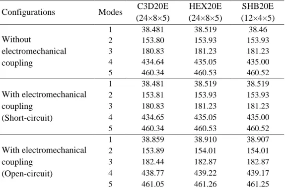
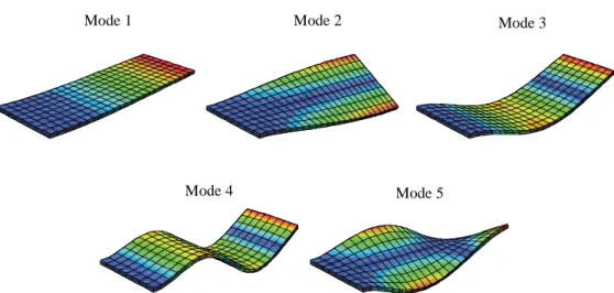
Figs. 4 shows the first five eigenmodes of vibration. The corresponding eigenfrequencies are reported in Table 3, where the results obtained with the SHB20E element are in excellent agreement with those given by the reference elements C3D20E and HEX20E. Also, one may notice the slight effect of electromechanical coupling on the natural frequencies. Indeed, the short-circuit configuration amounts to dealing with the case where the electromechanical
coupling is not accounted for. By contrast, when the circuit is open, the natural frequencies increase slightly. This increase in the eigenfrequencies is related to the resulting stiffness matrix, which becomes slightly stiffer due to electromechanical coupling. This phenomenon will be advantageously used in the sequel for the reduction and the control of vibration amplitudes.
In what follows, the damping properties of the cantilever plate will be evaluated using the derivative proportional control law described as:
{ }
φ
φ
φ
φ
a =gd{ }
φ
φ
φ
φ
s +gv{ }
φ
φ
φ
φ
ɺs (26) where gd and gv denote, respectively, the direct and velocity control gains. Accordingly, the associated control function H(ω
) can be expressed as:)
( d v
H
ω
= g +i gω
(27)The obtained results are presented in Figs. 5 and 6 for different values of the control gain and the loss factor. A first observation is that the obtained results are in perfect agreement with those given by reference elements. In addition, it should be pointed out that fewer degrees of freedom (DOFs) are required for the proposed SHB20E element (i.e., 5548 DOFs) to achieve results equivalent to those yielded by the HEX20E element (i.e., 19884 DOFs). Furthermore, the number of integration points used in the proposed solid–shell formulation is also much lower due to the adopted reduced-integration scheme.
More importantly, these graphs show the influence of the active control on the damping properties of the structure. Indeed, it initially appears that by increasing the direct gain parameter, the damped frequency increases overall up to a certain value of the damping coefficient. This increase is due to the increase in the stiffness matrix. However, beyond a certain value of the damping coefficient and of the direct gain parameter, the frequency starts to decrease, since the stiffness decreases as well. At the same time, the loss factor remains almost constant since the direct gain parameter does not induce any loss of energy.
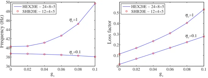
Concerning the velocity gain, a small variation of the frequency is observed for a low damping coefficient, while a more significant increase is obtained for high damping coefficients. On the other hand, the loss factor increases with the velocity gain and with the damping coefficient. Indeed, the velocity gain control law looks much like that of the viscoelastic dissipation, which explains the contribution to damping of the velocity gain.
In conclusion, this first test allowed us to highlight the interest as well as some limitations of this type of active vibration control. In order to enhance the active control, more complex laws, such as those resulting from a filter for instance, can be of considerable usefulness. In addition, it is sometimes important to engineers to have an idea of the amplitudes of
vibrations. To this end, frequency responses need to be computed, which will be done in the subsequent benchmark tests.
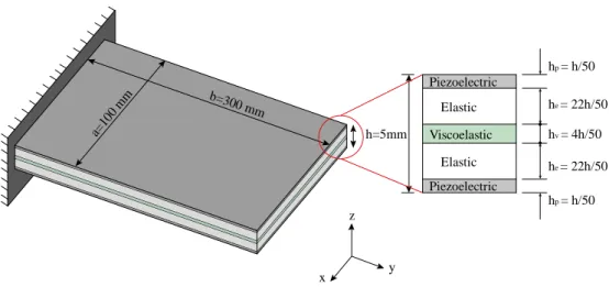
5.1.2. Frequency response of a sandwich plate in active-passive control
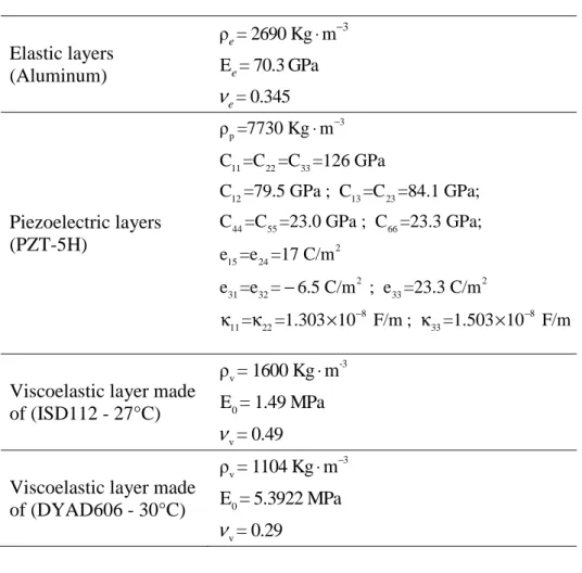
We consider now a rectangular plate on simple supports, as shown in Fig. 7. The piezoelectric faces are made of PZT-5H whose properties are given in Table 4. Two viscoelastic materials are used in the core in order to compare their effectiveness and to show their respective influence on active control. These viscoelastic materials consist of ISD112 - 27°C and DYAD606 - 30°C, whose behavior is described by the generalized Maxwell model:
( )
0 1 1 n j j j G G iω
ω
ω
= ∆ = + − Ω ∑
n=3 for ISD112 n=5 for DYAD606 (28)where G0 represents the shear modulus of delayed elasticity, while (∆ Ωj, j) are the parameters of the generalized Maxwell model given in Tables 5 and 6. The other mechanical parameters and piezoelectric properties are indicated in Table 4.
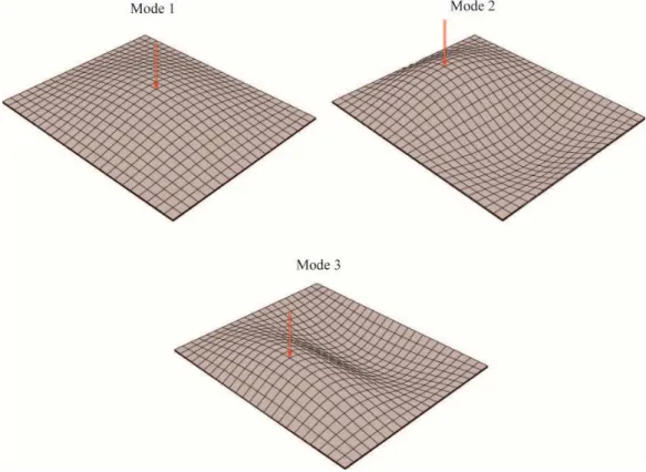
The elastic layers are made of aluminum. The first three modes of vibration will be investigated in order to reveal the interest as well as potential limitations of the different methods of control with respect to vibration modes.
A sinusoidal pulse of amplitude F =1000N is applied to excite the first three modes of vibration of the plate, as shown in Fig. 8. A combination of direct and velocity control gain parameters gd and gv, respectively, is adopted in order to disclose their respective contribution to the reduction of the amplitudes of vibrations for the different modes.
The simulation results in terms of amplitudes of vibrations for the first three modes are shown in Figs. 9–14. Once again, from computational efficiency perspective, the proposed piezoelectric solid–shell finite element SHB20E requires 4 times less degrees of freedom to provide results equivalent to those given by the reference element HEX20E. Moreover, the analysis of the frequency response curves allows us to better understand the influence of the various parameters for controlling the amplitudes of vibrations. It is concluded that the proportional derivative type control makes it possible to reduce more or less the amplitudes of vibrations for these two viscoelastic materials over all the excited modes. It should be noted that the choice of the values given to gd and gv is motivated by obtaining equivalent amplitude reductions. Thus, for the plate whose viscoelastic core is made of ISD112, the amplitude of vibration is reduced by approximately 30 to 40% compared to the use of passive control alone. As to the plate with viscoelastic layer made of DYAD606, the amplitudes of vibration are virtually all attenuated.
These analyzes make it possible to highlight all the difficulty in choosing a control law capable of attenuating all modes of vibration, whatever the viscoelastic material considered. Certainly models of optimal active control, such as LQR, LQG, etc., exist in the literature and provide interesting results. Nevertheless, other means such as the addition of filters in the control circuit may provide different alternatives. In order to investigate this, we propose hereafter active control laws presenting significant frequency dependence. The resolution of the corresponding equations will allow us, on the one hand, to validate the developed resolution tool and, on the other hand, to show the greater reduction in the amplitudes of vibrations by such laws.
5.2. Application to vibration amplitude reduction for sandwich plates
In this section, two retroactive control laws are applied to sandwich structures to control the amplitudes of vibrations. The first objective is to show the interest of using transfer filters and their contribution to the control of vibration amplitudes of structures. The second objective is to highlight the usefulness of the developed numerical tool in the consideration of nonlinear control laws.
5.2.1. Control with Gauss filter
We consider again the structure schematized in Fig. 7. A filter of Gaussian type is added to the circuit connecting the sensors to the actuators. The control law described by the function of this filter is given by the relation:
( )
0 2 exp i ; 100 Hω
kω
kω
= = (29)in which ω represents the frequency dependence, and
ω
0 is the natural frequency of the mode around which the analysis is performed. The first three modes are also excited by a force F =1000N. The amplitudes obtained with this law are superimposed to those obtained by passive damping and represented in Figs. 15–20. To check the validity of these results, we also compare the results obtained with the proposed solid–shell element SHB20E to those given by the HEX20E (quadratic hexahedral solid element). Once again, the results yielded by the solid–shell finite element SHB20E are in good agreement with those given by the HEX20E reference element, while the latter requires 4 times more degrees of freedom. Also, the analysis of Figs. 15–20 shows a reduction in maximum amplitudes ranging from 40% (for mode 1) to 60% (for mode 3), as compared to the passive control obtained by ISD112 - 27°C. For a sandwich plate whose core is made of DYAD606 - 30°C, this reduction varies between 20% (for mode 1) and 60% (for mode 3). The variation of coefficient k , which is involved in the filter function given by Eq. (29), may enable one to modulate the amplitude control.In order to improve the active control, another filter is placed in the active control circuit connecting the sensors to the piezoelectric actuators.
5.2.2. Control with Chebyshev filter
We consider again the same configuration as above, except for the control law, which is now described by the following relationship:
0 0 1 ( a b cos ; a , b and 0.65 a ) i H
ω
kω
ω
kω
= + = = = − (30)The frequency responses depicted in Figs. 21–26 show excellent agreement between the reference results provided by the HEX20E element and those obtained with the proposed solid–shell element SHB20E, with the latter necessitating once again 4 times less degrees of freedom for the same accuracy. Moreover, a much more significant attenuation of the amplitudes of vibrations is obtained with the Chebyshev filter, whatever the viscoelastic material used for the passive control. Therefore, this type of filter can be used in structures where no deflection is allowed, such as printed circuits where even a small deformation may cause malfunction of the device in which they are embedded.
6. Conclusions
In this work, a methodology, as well as the associated numerical simulation tools, has been proposed for active-passive control of vibrations. This is made possible thanks to the combination of the passive damping capabilities afforded by viscoelastic materials with the active control properties associated with piezoelectric materials. The main originality in the current contribution lies in the use of a filter-based controller to modulate the vibration amplitudes. For the modeling of the proposed system, a method is devised, which is based on the coupling of finite element discretization using a recently developed piezoelectric solid– shell element with the DIAMANT approach.
The extraction of the damping properties has been performed by extending the generic tool coupling the homotopy technique to the Asymptotic Numerical Method, which has been automated with the help of the Automatic Differentiation. The frequency responses of vibrations have been determined by a new Asymptotic Numerical Method, especially designed for active-passive vibration control. Then, a set of selective and representative vibration control tests have been successfully carried out, mainly on sandwich plate structures. In a preliminary step, the interest of active control has been shown by the use of the Proportional Derivative law for different damping coefficient values
η
c. To proceed further, two viscoelastic materials, the behavior of which depends on the frequency, have been introduced and the influence of two parameters, namely the direct and velocity control gains gd and gv, has been investigated. Finally, nonlinear active control laws, which exhibit significant frequency dependence, have been introduced with their advantages demonstrated in terms of allowed reduction of amplitudes of vibrations. These tests, although applied here mainly to sandwich plate structures, can also be extended to structures with more complex geometries.References
[1] E. M. Daya and M. Potier-Ferry, "A numerical method for nonlinear eigenvalue problems application to vibrations of viscoelastic structures," Computers & Structures, vol. 79, pp. 533-541, 2001.
[2] M. Bilasse, E. M. Daya, and L. Azrar, "Linear and nonlinear vibrations analysis of viscoelastic sandwich beams," Journal of Sound and Vibration, vol. 329, pp. 4950-4969, 2010.
[3] N. Jacques, E. M. Daya, and M. Potier-Ferry, "Nonlinear vibration of viscoelastic sandwich beams by the harmonic balance and finite element methods," Journal of
Sound and Vibration, vol. 329, pp. 4251-4265, 2010.
[4] A. J. M. Ferreira, A. L. Araújo, A. M. A. Neves, J. D. Rodrigues, E. Carrera, M. Cinefra, and C. M. Mota Soares, "A finite element model using a unified formulation for the analysis of viscoelastic sandwich laminates," Composites Part B: Engineering, vol. 45, pp. 1258-1264, 2013.
[5] W.-Y. Jung and A. J. Aref, "A combined honeycomb and solid viscoelastic material for structural damping applications," Mechanics of Materials, vol. 35, pp. 831-844, 2003. [6] Z. Li, "Vibration and acoustical properties and sandwich composite materials, PhD
Thesis," PhD Thesis, Auburn University, USA, 2006.
[7] R. Zhou and J. M. Crocker, "Effects of Thickness on Damping in Foam-filled Honeycomb-core Sandwich Beams," presented at the IMAC-XXV: Conference & Exposition on Structural Dynamics, 2007.
[8] K. Akoussan, H. Boudaoud, E. M. Daya, Y. Koutsawa, and E. Carrera, "Sensitivity analysis of the damping properties of viscoelastic composite structures according to the layers thicknesses," Composite Structures, vol. 149, pp. 11-25, 2016.
[9] K. Akoussan, H. Boudaoud, E. M. Daya, Y. Koutsawa, and E. Carrera, "Numerical method for nonlinear complex eigenvalues problems depending on two parameters: Application to three-layered viscoelastic composite structures," Mechanics of Advanced
Materials and Structures, DOI: 10.1080/15376494.2017.1286418, 2017.
[10] M. Filippi, E. Carrera, and A. M. Regalli, "Layerwise Analyses of Compact and Thin-Walled Beams Made of Viscoelastic Materials," Journal of Vibration and Acoustics, vol. 138, pp. 064501-064501-9, 2016.
[11] E. Carrera, "Developments, ideas, and evaluations based upon Reissner’s Mixed Variational Theorem in the modeling of multilayered plates and shells," Applied
Mechanics Reviews, vol. 54, pp. 301-329, 2001.
[12] E. Carrera, "Theories and Finite Elements for Multilayered Plates and Shells: A Unified compact formulation with numerical assessment and benchmarking," Archives of
Computational Methods in Engineering, vol. 10, pp. 215-296, 2003.
[13] E. Carrera, M. Cinefra, M. Petrolo, and E. Zappino, Finite element analysis of structures
[14] A. Shahdin, L. Mezeix, C. Bouvet, J. Morlier, and Y. Gourinat, "Fabrication and mechanical testing of glass fiber entangled sandwich beams: A comparison with honeycomb and foam sandwich beams," Composite Structures, vol. 90, pp. 404-412, 2009.
[15] E. Piollet, "Nonlinear damping of sandwich structures with core material made from entangled fibers," PhD Thesis, Université de Toulouse, France, 2014.
[16] K. G. Lougou, "Multiscale methods for the vibration modeling of structures with viscoelastic composite materials," PhD Thesis, Université de Lorraine, France, 2015. [17] S. C. Huang, D. J. Inman, and E. M. Austin, "Some design considerations for active and
passive constrained layer damping treatments," Smart Materials and Structures, vol. 5, pp. 301-313, 1996.
[18] M. J. Lam, D. J. Inman, and W. R. Saunders, "Vibration Control through Passive Constrained Layer Damping and Active Control," Journal of Intelligent Material
Systems and Structures, vol. 8, pp. 663-677, 1997.
[19] L. Duigou-Kersulec, "Numerical modeling of passive and active damping of sandwich structures with viscoelastic or piezoelectric layers," PhD Thesis, Université Paul Verlaine de Metz, France, 2002.
[20] H. Boudaoud, "Modeling of passive-active damping of sandwich structures," PhD Thesis, Université Paul Verlaine de Metz, France, 2007.
[21] M. Killpack and F. Abed-Meraim, "Limit-point buckling analyses using solid, shell and solid-shell elements," Journal of Mechanical Science and Technology, vol. 25, pp. 1105-1117, 2011.
[22] V.-D. Trinh, F. Abed-Meraim, and A. Combescure, "A new assumed strain solid-shell formulation “SHB6” for the six-node prismatic finite element," Journal of Mechanical
Science and Technology, vol. 25, pp. 2345-2364, 2011.
[23] A. Salahouelhadj, F. Abed-Meraim, H. Chalal, and T. Balan, "Application of the continuum shell finite element SHB8PS to sheet forming simulation using an extended large strain anisotropic elastic–plastic formulation," Archive of Applied Mechanics, vol. 82, pp. 1269-1290, 2012.
[24] P. Wang, H. Chalal, and F. Abed-Meraim, "Quadratic solid–shell elements for nonlinear structural analysis and sheet metal forming simulation," Computational Mechanics, pp. DOI: 10.1007/s00466-016-1341-8, 2016.
[25] Y. Koutsawa, I. Charpentier, E. M. Daya, and M. Cherkaoui, "A generic approach for the solution of nonlinear residual equations. Part I: The Diamant toolbox," Computer
Methods in Applied Mechanics and Engineering, vol. 198, pp. 572-577, 2008.
[26] M. Bilasse, I. Charpentier, E. M. Daya, and Y. Koutsawa, "A generic approach for the solution of nonlinear residual equations. Part II: Homotopy and complex nonlinear eigenvalue method," Computer Methods in Applied Mechanics and Engineering, vol. 198, pp. 3999-4004, 2009.
[27] K. Lampoh, I. Charpentier, and E. M. Daya, "A generic approach for the solution of nonlinear residual equations. Part III: Sensitivity computations," Computer Methods in
Applied Mechanics and Engineering, vol. 200, pp. 2983-2990, 2011.
[28] F. Kpeky, "Formulation and modeling of vibrations using solid-shell finite elements: application to viscoelastic and piezoelectric sandwich structures, PhD Thesis," PhD Thesis, Université de Lorraine, France, 2016.
[29] F. Kpeky, F. Abed-Meraim, H. Boudaoud, and E. M. Daya, "Linear and quadratic solid– shell finite elements SHB8PSE and SHB20E for the modeling of piezoelectric sandwich structures," Mechanics of Advanced Materials and Structures, DOI: 10.1080/15376494.2017.1285466, 2017.
[30] F. Abed-Meraim, V. D. Trinh, and A. Combescure, "New quadratic solid-shell elements and their evaluation on linear benchmark problems," Computing, vol. 95, pp. 373-394, 2013.
[31] H. Allik and T. J. R. Hughes, "Finite element method for piezoelectric vibration,"
International Journal for Numerical Methods in Engineering, vol. 2, pp. 151-157, 1970. [32] Z. C. Qiu, X. M. Zhang, H. X. Wu, and H. H. Zhang, "Optimal placement and active
vibration control for piezoelectric smart flexible cantilever plate," Journal of Sound and
Vibration, vol. 301, pp. 521-543, 2007.
[33] D. Chhabra, G. Bhushan, and P. Chandna, "Optimal Placement of Piezoelectric Actuators on Plate Structures for Active Vibration Control Using Modified Control Matrix and Singular Value Decomposition Approach," International Journal of
Mechanical, Aerospace, Industrial, Mechatronics and Manufacturing Engineering, vol. 7, pp. 458-463, 2013.
[34] F. Bachmann, A. E. Bergamini, and P. Ermanni, "Optimum piezoelectric patch positioning: A strain energy-based finite element approach," Journal of Intelligent
Material Systems and Structures, vol. 23, pp. 1575-1591, 2012.
[35] S. Wang, S.-T. Quek, and K. K. Ang, "LQR vibration control of piezoelectric composite plates," in Proc. SPIE 4235, Smart Structures and Devices, 2001, pp. 375-386.
[36] Z. Jingjun, H. Lili, W. Ercheng, and G. Ruizhen, "A LQR Controller Design for Active Vibration Control of Flexible Structures," in Computational Intelligence and Industrial
Application, Pacific-Asia Workshop, 2008, pp. 127-132.
[37] S. Q. Zhang and R. Schmidt, "LQR Control for Vibration Suppression of Piezoelectric Integrated Smart Structures," Proceedings in Applied Mathematics and Mechanics, vol. 12, pp. 695-696, 2012.
[38] B. Jemai, M. N. Ichchou, L. Jezequel, and M. Noe, "Comparison between a large bandwidth LQG and modal controlmethods applied to complex flexible structure," presented at the 2nd International Conference on Active Control in Mechanical Engineering, , Lyon, France, 1997.
[39] M. A. Trindade, A. Benjeddou, and R. Ohayon, "Piezoelectric Active Vibration Control of Damped Sandwich Beams," Journal of Sound and Vibration, vol. 246, pp. 653-677, 2001.
[40] P. Bildestein. (1990) Transfer functions for electric filters. Techniques de l’Ingénieur. [41] L. Azrar, E. H. Boutyour, and M. Potier-Ferry, "Non-linear forced vibrations of plates
by an Asymptotic-Numerical Method," Journal of Sound and Vibration, vol. 252, pp. 657-674, 2002.
[42] L. Azrar, S. Belouettar, and J. Wauer, "Nonlinear vibration analysis of actively loaded sandwich piezoelectric beams with geometric imperfections," Computers & Structures, vol. 86, pp. 2182-2191, 2008.
[43] F. Abdoun, L. Azrar, E. M. Daya, and M. Potier-Ferry, "Forced harmonic response of viscoelastic structures by an asymptotic numerical method," Computers & Structures, vol. 87, pp. 91-100, 2009.
[44] A. Elhage-Hussein, M. Potier-Ferry, and N. Damil, "A numerical continuation method based on Padé approximants," International Journal of Solids and Structures, vol. 37, pp. 6981-7001, 2000.
[45] B. Cochelin, N. Damil, and M. Potier-Ferry, Asymptotic numerical method, Hermes, Science Publications ed., 2007.
Tables
Table 1. Explicit forms for the matrices and vectors resulting from the electromechanical coupling. T uu u u V
ρ
dv = M ∫
N N Mass matrix[ ]
T uu u u V dv = K ∫
B C B Stiffness matrix[ ]
T V dv φφ φ φ = − K ∫
B κκκκ B Dielectric matrix[ ]
; T T u u u u T V dv φ φ φ φ = = K
∫
B e B K K Piezoelectric coupling matrix{ }
{ }
{ }
T T u u v s p V dv S ds =∫
+∫
+ F N f N f f Force vector{ }
{ }
{ }
T T v s p V dv S ds φ φ = −∫
−∫
−Q N q N q q Electrical charge vector
Table 2. Mechanical and piezoelectric properties of materials.
Elastic layers 3 ρ = 2040 Kg m E = 45.54 GPa = 0.33 e e e ν − ⋅ Piezoelectric layers (PZT4) p 11 22 33 13 23 12 44 55 66 2 15 24 2 2 31 32 33 8 11 22 33 3 ρ =7500 Kg m C =C =139 GPa ; C =115.3 GPa C =C =74.3 GPa ; C =77.8 GPa C =C =25.6 GPa ; C =30.6 GPa e =e =12.7 C/m e =e = 5.21 C/m ; e =15.1 C/m = =1.31 10 F/m ; =1.15 10 − − − ⋅ − κ κ × κ × 8 F/m Viscoelastic layer 3 v 0 v ρ = 1200 Kg m E = 7.25 MPa = 0.45 ν − ⋅
Table 3. First five eigenfrequencies for the five-layer cantilever sandwich plate.
Configurations Modes C3D20E (24×8×5) HEX20E (24×8×5) SHB20E (12×4×5) Without electromechanical coupling 1 38.481 38.519 38.46 2 153.80 153.93 153.93 3 180.83 181.23 181.23 4 434.64 435.05 435.00 5 460.34 460.53 460.52 With electromechanical coupling (Short-circuit) 1 38.481 38.519 38.519 2 153.81 153.93 153.93 3 180.83 181.23 181.23 4 434.65 435.05 435.00 5 460.34 460.53 460.52 With electromechanical coupling (Open-circuit) 1 38.859 38.910 38.907 2 153.89 154.01 154.01 3 182.44 182.87 182.87 4 438.77 439.22 439.17 5 461.05 461.26 461.25
Table 4. Mechanical and piezoelectric properties of materials. Elastic layers (Aluminum) 3 ρ = 2690 Kg m E = 70.3 GPa = 0.345 e e e ν − ⋅ Piezoelectric layers (PZT-5H) 3 p 11 22 33 12 13 23 44 55 66 2 15 24 2 2 31 32 33 8 8 11 22 33 ρ =7730 Kg m C =C =C =126 GPa C =79.5 GPa ; C =C =84.1 GPa; C =C =23.0 GPa ; C =23.3 GPa; e =e =17 C/m e =e = 6.5 C/m ; e =23.3 C/m = =1.303 10 F/m ; =1.503 10 F/m − − − ⋅ − κ κ × κ ×
Viscoelastic layer made of (ISD112 - 27°C) -3 v 0 v ρ = 1600 Kg m E = 1.49 MPa = 0.49 ν ⋅
Viscoelastic layer made of (DYAD606 - 30°C) 3 v 0 v ρ = 1104 Kg m E = 5.3922 MPa = 0.29 ν − ⋅
Table 5. Viscoelastic parameters for ISD112 - 27°C.
j ∆j -1 (rad.s ) j Ω 1 0.746 468.7 2 3.265 4742.4 3 43.284 71532.5
Table 6. Viscoelastic parameters for DYAD606 - 30°C.
j ∆j -1 (rad.s ) j Ω 1 5.40 73.06 2 14.15 453.34 3 1.43 8.83 4 28.33 3406.80 5 128.85 52781.28
Figures
Figure 1. Schematic representation for the reference geometry of the SHB20E element as well as for the location of its integration points in the case when the number of through-thickness
integration points is nint=3.
Figure 2. Active-passive damping system using a viscoelastic material and piezoelectric layers with filter controller.
Figure 3. Five-layer cantilever sandwich plate with viscoelastic core and piezoelectric faces.
ux6 uy6 uz 6 ɸ6 2 3 1 4 6 7 5 20 8 9 10 11 12 17 13 19 14 15 16 18 ξ η ζ 1 2 3 4 5 6 7 8 9 10 11 12 Controller (Filter) Viscoelastic Piezoelectric Piezoelectric Elastic Elastic Sensor (s) Actuator (a) Piezoelectric Elastic Viscoelastic Elastic Piezoelectric hp= h/50 he= 22h/50 hv= 4h/50 hp= h/50 he= 22h/50 x y z b=300 mm a=10 0 m m h=5mm
Figure 4. First five eigenmodes for the five-layer cantilever sandwich plate.
Figure 5. Damping parameters with variation of the direct control gain gd (gv =0).
Mode 1 Mode 2 Mode 3
Mode 4 Mode 5 −30 −20 −10 0 10 20 30 20 25 30 35 40 45 gd F re q u e n c y ( H z ) HEX20E − 24×8×5 SHB20E − 12×4×5 ηc=0.1 ηc=1 −300 −20 −10 0 10 20 30 0.06 0.03 0.09 0.12 0.15 gd L o ss f a c to r HEX20E − 24×8×5 SHB20E − 12×4×5 ηc=1 ηc=0.1
Figure 6. Damping parameters with variation of the velocity control gain gv (gd =0).
Figure 7. Simply supported five-layer sandwich plate.
HEX20E − 24×8×5 SHB20E − 12×4×5 0 0.02 0.04 0.06 0.08 0.1 36 38 40 42 44 46 48 50 gv F re q u e n c y ( H z ) ηc=1 ηc=0.1 HEX20E − 24×8×5 SHB20E − 12×4×5 0 0.02 0.04 0.06 0.08 0.1 0 0.1 0.2 0.3 0.4 0.5 gv L o ss f a c to r ηc=1 ηc=0.1 0.1 mm 0.1 mm 0.8 mm 0.8 mm 0.2 mm PZT-5H PZT-5H ISD112 or DYAD606 Aluminum Aluminum 300 mm 250 mm x y z
Figure 8. Loading applied to the plate for different excited modes.
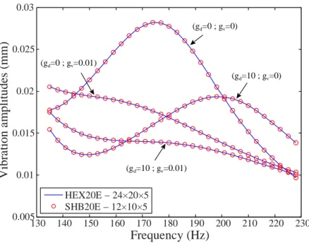
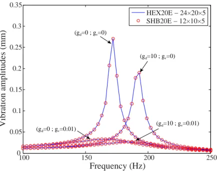
Figure 9. Frequency response with combination of the coefficients of the Proportional Derivative law (ISD112 - 27°C) – Mode 1.
(gd=10 ; gv=0.01) (gd=0 ; gv=0.01) (gd=10 ; gv=0) (gd=0 ; gv=0) 50 60 70 80 90 100 110 120 130 140 150 0.01 0.02 0.03 0.04 0.05 0.06 0.07 0.08 0.09 Frequency (Hz) V ib ra ti o n a m p li tu d es ( m m ) HEX20E − 24×20×5 SHB20E − 12×10×5
Figure 10. Frequency response with combination of the coefficients of the Proportional Derivative law (ISD112 - 27°C) – Mode 2.
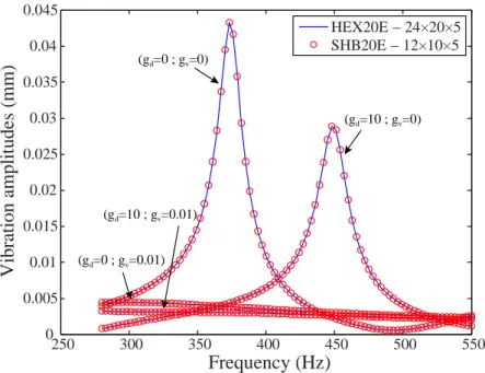
Figure 11. Frequency response with combination of the coefficients of the Proportional Derivative law (ISD112 - 27°C) – Mode 3.
(gd=10 ; gv=0.01) (gd=0 ; gv=0.01) (gd=10 ; gv=0) (gd=0 ; gv=0) HEX20E − 24×20×5 SHB20E − 12×10×5 130 140 150 160 170 180 190 200 210 220 230 0.005 0.01 0.015 0.02 0.025 0.03 Frequency (Hz) V ib ra ti o n a m p li tu d es ( m m ) (gd=10 ; gv=0.01) (gd=0 ; gv=0.01) (gd=10 ; gv=0) (gd=0 ; gv=0) HEX20E − 24×20×5 SHB20E − 12×10×5 140 160 180 200 220 240 260 280 0.006 0.008 0.01 0.012 0.014 0.016 0.018 0.02 0.022 Frequency (Hz) V ib ra ti o n a m p li tu d es ( m m )
Figure 12. Frequency response with combination of the coefficients of the Proportional Derivative law (DYAD606 - 30°C) – Mode 1.
Figure 13. Frequency response with combination of the coefficients of the Proportional Derivative law (DYAD606 - 30°C) – Mode 2.
100 150 200 250 0 0.05 0.1 0.15 0.2 0.25 0.3 0.35 Frequency (Hz) V ib ra ti o n a m p li tu d es ( m m ) (gd=10 ; gv=0.01) (gd=0 ; gv=0.01) (gd=10 ; gv=0) (gd=0 ; gv=0) HEX20E − 24×20×5 SHB20E − 12×10×5 200 250 300 350 400 450 0 0.01 0.02 0.03 0.04 0.05 0.06 0.07 Frequency (Hz) V ib ra ti o n a m p li tu d e s (m m ) (gd=10 ; gv=0.01) (gd=0 ; gv=0.01) (gd=10 ; gv=0) (gd=0 ; gv=0) HEX20E − 24×20×5 SHB20E − 12×10×5
Figure 14. Frequency response with combination of the coefficients of the Proportional Derivative law (DYAD606 - 30°C) – Mode 3.
Figure 15. Frequency response with ISD112 - 27°C and Gauss filter – Mode 1.
250 300 350 400 450 500 550 0 0.005 0.01 0.015 0.02 0.025 0.03 0.035 0.04 0.045 Frequency (Hz) V ib ra ti o n a m p li tu d e s (m m ) (gd=10 ; gv=0.01) (gd=0 ; gv=0.01) (gd=10 ; gv=0) (gd=0 ; gv=0) HEX20E − 24×20×5 SHB20E − 12×10×5 Passive damping Hybrid control (Gauss filter) 0 50 100 150 200 250 300 350 400 0 0.01 0.02 0.03 0.04 0.05 0.06 0.07 0.08 0.09 Frequency (Hz) V ib ra ti o n a m p li tu d es ( m m ) HEX20E − 24×20×5 SHB20E − 12×10×5
Figure 16. Frequency response with ISD112 - 27°C and Gauss filter – Mode 2.
Figure 17. Frequency response with ISD112 - 27°C and Gauss filter – Mode 3.
Passive damping Hybrid control (Gauss filter) HEX20E − 24×20×5 SHB20E − 12×10×5 0 50 100 150 200 250 300 350 400 0 0.005 0.01 0.015 0.02 0.025 0.03 0.035 0.04 0.045 0.05 Frequency (Hz) V ib ra ti o n a m p li tu d es ( m m ) Passive damping Hybrid control (Gauss filter) HEX20E − 24×20×5 SHB20E − 12×10×5 0 50 100 150 200 250 300 350 400 0 0.005 0.01 0.015 0.02 0.025 0.03 0.035 0.04 0.045 Frequency (Hz) V ib ra ti o n a m p li tu d e s (m m )
Figure 18. Frequency response with DYAD606 - 30°C and Gauss filter – Mode 1.
Figure 19. Frequency response with DYAD606 - 30°C and Gauss filter – Mode 2.
0 50 100 150 200 250 300 350 400 0 0.05 0.1 0.15 0.2 0.25 0.3 0.35 Frequency (Hz) V ib ra ti o n a m p li tu d es ( m m ) Passive damping Hybrid control (Gauss filter) HEX20E − 24×20×5 SHB20E − 12×10×5 0 50 100 150 200 250 300 350 400 0 0.02 0.04 0.06 0.08 0.1 0.12 Frequency (Hz) V ib ra ti o n a m p li tu d es ( m m ) Passive damping Hybrid control (Gauss filter) HEX20E − 24×20×5 SHB20E − 12×10×5
Figure 20. Frequency response with DYAD606 - 30°C and Gauss filter – Mode 3.
Figure 21. Frequency response with ISD112 - 27°C and Chebyshev filter – Mode 1.
0 50 100 150 200 250 300 350 400 0 0.02 0.04 0.06 0.08 0.1 0.12 Frequency (Hz) V ib ra ti o n a m p li tu d es ( m m ) Passive damping Hybrid control (Gauss filter) HEX20E − 24×20×5 SHB20E − 12×10×5 Passive damping Hybrid control (Chebyshev filter) HEX20E − 24×20×5 SHB20E − 12×10×5 0 50 100 150 200 250 300 350 400 0 0.01 0.02 0.03 0.04 0.05 0.06 0.07 0.08 0.09 Frequency (Hz) V ib ra ti o n a m p li tu d e s (m m )
Figure 22. Frequency response with ISD112 - 27°C and Chebyshev filter – Mode 2.
Figure 23. Frequency response with ISD112 - 27°C and Chebyshev filter – Mode 3.
0 Passive damping Hybrid control (Chebyshev filter) HEX20E − 24×20×5 SHB20E − 12×10×5 0 50 100 150 200 250 300 350 400 0.005 0.01 0.015 0.02 0.025 0.03 0.035 0.04 0.045 0.05 Frequency (Hz) V ib ra ti o n a m p li tu d e s (m m ) Passive damping Hybrid control (Chebyshev filter) HEX20E − 24×20×5 SHB20E − 12×10×5 0 50 100 150 200 250 300 350 400 0.005 0.01 0.015 0.02 0.025 0.03 0.035 0.04 0.045 Frequency (Hz) V ib ra ti o n a m p li tu d es ( m m )