Fractal Dimension of Grain Boundary during Heating. Comparison between Images Analyses and Monte Carlo Simulation

Science Arts & Métiers (SAM)

is an open access repository that collects the work of Arts et Métiers Institute of Technology researchers and makes it freely available over the web where possible.

This is an author-deposited version published in: https://sam.ensam.eu

Handle ID: .http://hdl.handle.net/10985/9729

To cite this version :

Maxence BIGERELLE, J. FAVERGEON, Alain IOST - Fractal Dimension of Grain Boundary during Heating. Comparison between Images Analyses and Monte Carlo Simulation - Defect and Diffusion Forum - Vol. 323-325, p.133-138 - 2012

Any correspondence concerning this service should be sent to the repository Administrator : archiveouverte@ensam.eu

Science Arts & Métiers (SAM)

is an open access repository that collects the work of Arts et Métiers ParisTech researchers and makes it freely available over the web where possible.

This is an author-deposited version published in: http://sam.ensam.eu

Handle ID: .http://hdl.handle.net/null

To cite this version :

Maxence M BIGERELLE, J FAVERGEON, Alain IOST - Fractal Dimension of Grain Boundary during Heating. Comparison between Images Analyses and Monte Carlo Simulation - Defect and Diffusion Forum - Vol. 323-325, p.133-138 - 2012

Any correspondence concerning this service should be sent to the repository Administrator : archiveouverte@ensam.eu

Fractal Dimension of Grain Boundary during Heating.

Comparison between Images Analyses and Monte Carlo Simulation

M. Bigerelle

, J. Favergeon

and A.Iost

1

Laboratoire de Mécanique Roberval, UTC, UMR 6253, 60205 Compiègne, France

2

Arts et Metiers ParisTech ; LML, CNRS UMR 8107 ; ENSAM Lille, 8 boulevard Louis XIV, 59046 Lille Cedex, France.

3

UVHC, TEMPO EA 4542, F-59313 Valenciennes, France.

a

maxence.bigerelle@utc.fr, bjerome.favergeon@utc.fr, calain.iost@ensam.eu

Keywords: Monte-Carlo simulation, grain growth, fractal, diffusion.

Abstract. There are few articles that mention fractal dimension in grain growth mechanism. Some authors build a simplified analytic model showing that initial fractal dimension of grain boundary has an influence on interface modification velocity. Nevertheless they postulate the relation

∆

−

=_cs1

L where L is the grain length, c is a constant, s is grain size and ∆ the fractal dimension. The aims of this paper is to experimentally analyze by image analysis the fractal dimension of A5 aluminum sheet grain boundaries during heating and to simulate their evolution by a Monte Carlo method to validate experimental data.. It is shown by Monte-Carlo simulation and confirmed experimentally that the grain growth process decreases the fractal dimension of grain border. It can be concluded that it is very hazardous to build a model of grain growth without including the effect of grain’s morphology. The macroscopic fractal morphology of the grain structure could then be used to validate microscopic relation between Monte Carlo Steps time and real time.

Introduction

There are few articles that mention fractal dimension in grain growth mechanism; we noticed Rubio et al. [1], Tanaka [2-4] and Streitenberg et al. [5]. These authors build a simplified analytic model showing that initial grain boundariy fractal dimension has an influence on the interface modification velocity. Nevertheless they postulate the relation L=cs1−∆ where L is length of profile,

c is a constant, s is the grain size and ∆ the fractal dimension. The aims of this paper are to experimentally analyse the grain boundary fractal dimension of aluminum sheet during annealing and to simulate the heating process by a Monte-Carlo method to validate experimental data.

Analysis of aluminum during grain growth

Nine samples of aluminum (99.99 %) were annealed at 550±3°Cin ambient atmosphere after a plastic deformation of 3,0±0.2% (uniaxial traction rate of v = 1 mm.mn-1) for different heating times (1, 2, 4, 8, 16, 32, 64, 128 and 256 hours). To reveal microstructure, the samples were pickled with boiling soda then they were attacked with a solution containing nitric acid (45 %), fluoridric acid (15 %) and ethanol (40 %).

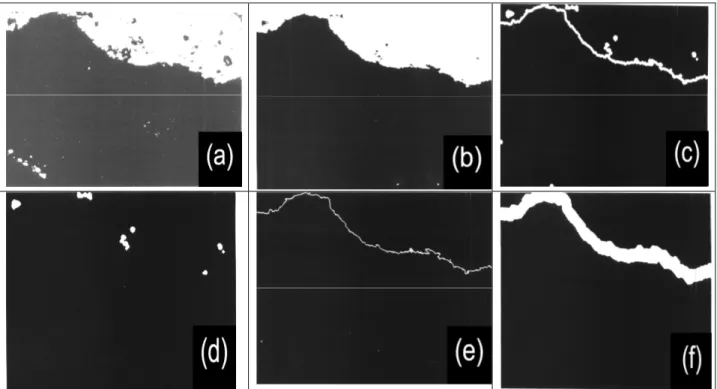
The grain boundaries are first digitalized with a 1024x1024 resolution CCD camera (Fig1.a). Eight measures were performed on different grains for the whole samples. Then the CCD images are transformed into a binary one thanks to a maximal entropy filter that leads to have one grain in white and the other grain in black (fig. 1.b). One has then to detect the grain boundary (fig.1.c). However, some isolated islands appear that must be suppressed. They are firstly isolated (fig.1d) and thanks to a subtraction with fig.1c, the final grain boundary is obtained on figure 1.e. Then evaluation of the fractal dimension of this interface is performed by the Minkowski method. This method consists in covering the grain boundary by a circle of radius, r (in image analyses this operation is called a

"dilatation") and to measure the area, A(r) of the dilated shape called the “Minkowski’s sausage” (fig 1.f).

Figure 1: Protocol of Fractal image analyses of the aluminium grain boundary. a) Image sampling (1024x1024) with 256 grey levels. b) Entropy treatment of image a (binary image). c) contours detection of image b. d) Non border shapes suppression of image c. e) Image c minus image d with skeleton transformation. f) Dilatation of image e (10 dilatations).

By covering the grain boundary by disks with radius r whose centers lie on the curve and varying the circle radius, one obtains different pair of

(

)

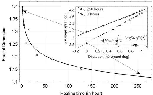
correlation relation for 2 h and 255 h heating times is shown on the included images of fig. 2. For every regression line, the slope standard deviation calculated with the Student theory is estimated to be 0.02. Thanks to the representation of the evolution of the fractal dimension with the annealing time (fig. 2) where every point is the mean of eight calculated fractal dimension we can say that the 95 % precision of every point is given by 2× 0.02 8≈0.015.

The very fast diminution of the fractal dimension with the annealing time has a logarithmic shape. The initial grain fractal dimension is 1.4 and becomes 1.12 after a 250 hour long annealing time and seems always decreasing after this time as a consequence of surface energy minimisation. Nevertheless the measure inaccuracy does not allow us to statistically assess this hypothesis. The fractal increment α with ∆ 2= −α was twice after 8 hours. To experimentally validate this hypothesis, 7 plastic deformations were performed varying from 6% to 16% and followed by a 550°C annealing during 45 hours. The grains size varies from 5.5 mm (6%) to 0.7 mm (13%). It is shown that the fractal dimension is nearly constant (see fig.3, right) and equals to 1.22.

Figure 2: Evolution of aluminium grain limit fractal dimension with annealing time. The curve is a logarithm regression with equation ∆=1.401−0.116logt_h. Each point is the mean of eight measures.

The insert represents the variation g of the sausage area with the dilatation increment for two annealing times. . Plastic deformation (%) G ra in d ia m e te r (m m ) 0.5 1.5 2.5 3.5 4.5 5.5 6.5 5 6 7 8 9 10 11 12 13 14 Plastic deformation (%) F rac tal dim ens ion 1.1 1.15 1.2 1.25 1.3 1.35 1.4 1.45 5 6 7 8 9 10 11 12 13 14 15 16 17 Plastic deformation (%) Gr a in d ia m e te r (m m ) 0.5 1.5 2.5 3.5 4.5 5.5 6.5 5 6 7 8 9 10 11 12 13 14

Figure 3. Left: Size of grains versus the plastic deformation (in %) for an annealing time of 45 hours at heating temperature of 550°C. Right: Evolution of fractal dimension of aluminum grain boundary

versus plastic deformation for the same annealing time of 45 hours at 550°C.

As a consequence, the grain boundary fractal dimension does not depend on the recrystallization mechanism introduced by plastic strain (and as a consequence, the initial grain sizes) and is only due to the diffusion process at the grain interfaces during grain growth.

Monte-Carlo simulation of fractal morphology grains interface during heating

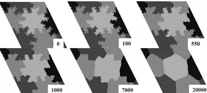
A Monte Carlo simulation is used to check if the grain boundary fractal dimension evolves with the annealing time. In order to validate this hypothesis, we created a paving with mathematical Von Koch curve which a 1.5 fractal dimension (initial picture of Fig.4).

Figure 4: Monte Carlo Simulation of grain boudary diffusion created with a Von Koch curve (1.5 fractal dimension, after 100, 550, 1000, 7000 and 20000 MCS.

A first “flake” curve is centred on the matrix, the other “flakes” curves are pinned in the image boundaries. This configuration allows us to only analyse the boundary fractal behaviour. The Monte-Carlo algorithm was proposed by Anderson et al. [6]. The grain structure is modelled in two dimensions. Each element of simulation box is a number zi called spin or orientation which value lies

between 1 and Q. Q represents the number of possible crystallographic orientations of a grain (in this simulation Q=4). Two adjacent numbers whith different spins constitute the grain boundary. We use a microscopic approach to quantify the real time of a Monte-Carlo elementary process applied to a FCC grid. We suppose that diffusion involving the grain growth is principally based on the self-diffusion while the interstitial diffusion is considered absent because of the high energy it needs in a compact structure. In a FCC structure with a mesh parameter called a, there are 12 possible jumps: 4 jumps with a −a 2 long projection, 4 jumps with a null projection and 4 jumps with and a long projection. The self-diffusion coefficient is given by the Einstein’s equation:

      + × + Γ = 4 4 0 4 4 4 2 1 _a2 _a2 D_{FCC S} (1)

where ΓS is the jump frequency from a site to another. If Γ is the mean jump frequency per time unit,

we have

12

2

a

D_FCC =Γ and then a jump corresponds to

FCC D a 12 1 2 = Γ seconds.

During a Monte-Carlo simulation, in a triangular structure with a mesh parameter called a', there are 6 possible jumps: 2 jumps with a a' long projection and 4 jumps with a a' 2 long projection. The diffusion coefficient is:

2 ' ' 3 ' 2 4 ' 4 2 1 2 2 2 ' a a a D S S MCS Γ =       + Γ = (2) And then D_MCS =Γ_S'a'2 4 (3)

As we suppose that the Monte-Carlo simulation is based on self-diffusion D_MCS =D_FCC . Moreover the number of spins has to be considered. In fact the jump probability also depends on Q. At the average, a jump happens at every MCS with the probability 1/Q. Thus Monte-Carlo iteration is

Saito [7, 8] found a similar expression ( QD a MCS 6 ' 1 2

= ). However he did not take into account the crystallographic structure. Moreover he did not explain the signification of D and did not experimentally validate his expression.

From the initial Von Koch curve (fig. 4) Monte-Carlo simulation we can notice the following conclusions:

1- The grain becomes less and less fractal as the Monte-Carlo steps increase. The diffusion process inverses the Von Koch curve building one.

2- The grain reaches a equilibrium structure that is the hexagonal shape, which is the basic one to build a Von Koch curve.

3- The grain area remains unchanged during Monte-Carlo steps.

In order to calculate the relation between real time and MCS time with equation (4), we have to impose a measure on a'. The mean size of the Von Koch curve we used was measured and its area remains constant during the MCS iterations. This curve mean size is 621 pixels and Q = 4. We statistically showed that the grain size is independent on the annealing time. Thus we used a 5 mm grain diameter. The aluminum mesh parameter is 4.04 Å and there are 12376237 meshes in a grain diameter. Consequently 1 pixel corresponds to 20000 meshes. The aluminum self-diffusion coefficient is given by Brebec [9] and reported by Philibert [10] 0.035exp 28750(CGS)

    ₋ = RT D_Alu

which gives here DFCC = 8.12 10-10 cm2.s-1 then:

(

)

Comparison Experimental data - Monte-Carlo simulation

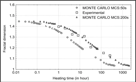
Figure 5 represents the fractal dimensions obtained by the Monte-Carlo method with real times and experimental ones.

As we are not able to experimentally determine the grain fractal dimension when grain growth starts, it is not possible to simulate the initial Von Koch curve. To estimate the initial Von Koch curve fractal dimension, an inverse method is proposed to obtain the real grain fractal dimension after a one hour long simulation. A very good correlation between the modelled values and the measured ones are found. Simulated curve only presents an horizontal shift of 0.05. The following observations can be made:

* The initial recrystallised grain fractal dimension before grain growth is unknown because only fractal dimension after one hour annealing is known. We supposed that the initial fractal dimension was 1.5. A higher initial fractal dimension would lead to a better correlation.

* There is a high uncertainty on the diffusion coefficient and the activation energy that we used. In fact, if we use the Stoebe’s et al. [11] value, the aluminum self-diffusion coefficient at 550°C would be 7.43 10-10 cm2.s-1 and the MCS time would be 54 seconds. If we use the Lundy’s and Murdock’s [12] value, the self-diffusion coefficient would be 15.97 10-10 cm2.s-1 and the MCS time would be 25 seconds. These self-diffusion coefficients are for very pure metal ones. If the structure would be heterogeneous, the diffusion coefficient would be modified. Poulsen et al. show that the activation energy for a single grain may shove substantial deviations from the grain-averaged activation energy for impurity-controlled recrystalisation of aluminium [13]. If we would use 200 seconds as the MCS time unit, the Monte-Carlo simulation representation would the same as the experimental data (fig. 5).

Heating time (in hour) F ra c ta l d im e n s io n 1 1.1 1.2 1.3 1.4 1.5 1.6 0.01 0.1 1 10 100 1000 MONTE CARLO MCS:50s Experimental MONTE CARLO MCS:200s

Figure 5: Evolution of Aluminum grain boundary fractal dimension annealed at 550°C achieved by : Simulation of diffusion mechanism on a Von Koch curve (dimension 1,5) with two different jump frequency (1MCS=200 seconds and 1 MCS=50 seconds) and measured experimentally with image

analyses. Conclusion

In this study we have shown by Monte-Carlo simulation and experimentally confirmed that the grain growth process decreases the fractal dimension of the grain boundary. We can conclude that it’s very hazardous to build a model of grain growth without including the effect of grain’s morphology. The macroscopic fractal morphology of the grain structure could then be used to validate microscopic relation with the between MCS time and real time.

Acknowledgements

This work was supported by the Région Picardie (France) and the FEDER (Fonds européen de développement régional) in the Project FoncRug3D.

References

[1] F. Rubio, J. Rubio and J. L. Oteo: J. Mat. Sci. Lett. Vol. 16 (1997), p. 49. [2] M. Tanaka and H. Lizuka: Z. Metallk. Vol 82 (1991), p. 442.

[3] M. Tanaka: J. Mat. Sci. Vol. 28 (1993), p. 5753. [4] M. Tanaka: J. Mat. Sci., Vol. 31 (1996), p. 3513.

[5] P. Streitenberger, D. Fôrster, G. Kolbe and P. Veit: Scripta Mat. Vol. 33 (1995), p. 541.

[6] M.P. Anderson, D.J. Srolovitz, G.S. Grest and P. S. Sahni: Acta Metall. Vol. 32 (1985), p. 783. [7] Y. Saito : Mat. Sci. Eng. A Vol. 223 (1997), p. 114.

[8] Y. Saito: ISIG Inter Vol. 38 (1998), p. 559.

[9] G. Brebec: in Mass transport in Solids, pp. 251-281, 1983.

[10] J. Philibert : Diffusion et transport de matière dans les solides, (Monographies de physique, Les Editions de Physique, France, 1985).

[11] T.G. Stoebe, R.D. Gulliver, T.0. Ogurtani and R.A. Huggins: Acta Metal. Vol. 13 (1965), p. 701. [12] T.S. Lundy and J. F. Murdock: J. Appl. Phys Vol. 33 (1962), p. 1671.

[13] S.O. Poulsen, E.M. Lauridsen, A. Lyckegaard, J. Oddershede, C. Gundlach, C. Curfs and D. Juul Jensen: Scripta Mat. Vol. 64 (2011), p. 1003