On the capacity of free-space optical intensity channels

HAL Id: tel-02266362

https://pastel.archives-ouvertes.fr/tel-02266362

Submitted on 14 Aug 2019

HAL is a multi-disciplinary open access

archive for the deposit and dissemination of sci-entific research documents, whether they are pub-lished or not. The documents may come from teaching and research institutions in France or abroad, or from public or private research centers.

L’archive ouverte pluridisciplinaire HAL, est destinée au dépôt et à la diffusion de documents scientifiques de niveau recherche, publiés ou non, émanant des établissements d’enseignement et de recherche français ou étrangers, des laboratoires publics ou privés.

Longguang Li

To cite this version:

Longguang Li. On the capacity of free-space optical intensity channels. Information Theory [cs.IT]. Université Paris-Saclay, 2019. English. �NNT : 2019SACLT028�. �tel-02266362�

Th

`ese

de

doctor

at

NNT

:2019SA

CL

T028

On the Capacity of Free-Space Optical

Intensity Channels

pr´epar´ee `a T´el´ecom ParisTech Ecole doctorale n 528: sciences et technologies de l’information et de la communication (STIC)

Sp´ecialit´e de doctorat : r´eseaux, information et communications

Th`ese pr´esent´ee et soutenue `a Paris, le 13 Juillet 2019, par

L

L

Composition du Jury : M. Philippe Ciblat

Professeur, T´el´ecom ParisTech Pr´esident M. Amos Lapidoth

Professeur, ETH Zurich Rapporteur M. Andrew Eckford

Professeur, York University Rapporteur M. Ligong Wang

Charg´e de recherche, CNRS Examinateur Mme Lina Mroueh

Maˆıtre de Conf´erences, Institut Sup´erieur d’Electronique de Paris Examinateur Mme Mich`ele Wigger

Professeur, T´el´ecom ParisTech Directeur de th`ese M. Stefan Moser

Titre : Sur la Capacité des Canaux d’Intensité Optique en Espace Libre

Mots clés : Capacité des Canaux, Communication d’Intensité Optique, Entrées Multiples et Sorties Multiples

(MIMO)

Résumé : Les systèmes de communication à

in-tensité optique en espace libre (FSOI) sont large-ment utilisés dans les communications à courte por-tée, telles que les communications infrarouges entre des dispositifs électroniques portables. L’émetteur de ces systèmes module sur l’intensité des signaux optiques émis par des diodes électroluminescentes (LEDs) ou des diodes laser (LDs), et le récepteur me-sure les intensités optiques entrantes au moyen de photodétecteurs. Les entrées ne sont pas négatives car elles représentent des intensités. En outre, ils sont généralement soumis à des contraintes de sance de pointe et moyenne, la contrainte de puis-sance de pointe étant principalement dû aux limita-tions techniques des composants utilisés, alors que la contrainte de puissance moyenne est imposée par des limitations de batterie et des considérations de sécurité. En première approximation, le bruit dans de tels systèmes peut être supposé être gaussien et in-dépendant du signal transmis.

Cette thèse porte sur les limites fondamentales des systèmes de communication FSOI, plus précisément sur leur capacité. L’objectif principal de notre travail est d’étudier la capacité d’un canal FSOI général à en-trées multiples et sorties multiples (MIMO) avec une contrainte de puissance de crête par entrée et une contrainte de puissance moyenne totale sur toutes les antennes d’entrée. Nous présentons plusieurs résul-tats de capacité sur le scénario quand il y a plus d’an-tennes d’émission que d’and’an-tennes de réception,

c’est-à-dire, nT> nR> 1. Dans ce scénario, différents vec-teurs d’entrée peuvent donner des distributions iden-tiques à la sortie, lorsqu’ils aboutissent au même vec-teur d’image multiplié par la matrice de canal. Nous déterminons d’abord les vecteurs d’entrée d’énergie minimale permettant d’atteindre chacun de ces vec-teurs d’image. Il définit à chaque instant dans le temps un sous-ensemble de nT nR antennes à zéro ou à pleine puissance et utilise uniquement les nR an-tennes restantes pour la signalisation. Sur cette base, nous obtenons une expression de capacité équiva-lente en termes de vecteur d’image, ce qui permet de décomposer le canal d’origine en un ensemble de canaux presque parallèles. Chacun des canaux paral-lèles est un canal MIMO nR⇥ nRà contrainte d’ampli-tude, avec une contrainte de puissance linéaire, pour laquelle des limites de capacité sont connues. Avec cette décomposition, nous établissons de nouvelles limites supérieures en utilisant une technique de li-mite supérieure basée sur la dualité, et des lili-mites inférieures en utilisant l’inégalité de puissance d’en-tropie (EPI). Les limites supérieure et inférieure déri-vées correspondent lorsque le rapport signal sur bruit (SNR) tend vers l’infini, établissant la capacité asymp-totique à haut SNR. À faible SNR, il est connu que la pente de capacité est déterminée par la trace maxi-male de la matrice de covariance du vecteur image. Nous avons trouvé une caractérisation de cette trace maximale qui est plus facile à évaluer en calcul que les formes précédentes.

Abstract : Free-space optical intensity (FSOI)

com-munication systems are widely used in short-range communication such as the infrared communication between electronic handheld devices. The transmit-ter in these systems modulates on the intensity of op-tical signals emitted by light emitting diodes (LEDs) or laser diodes (LDs), and the receiver measures in-coming optical intensities by means of photodetec-tors. Inputs are nonnegative because they represent intensities. Moreover, they are typically subject to both peak- and average-power constraints, where the peak-power constraint is mainly due to techni-cal limitations of the used components, whereas the average-power constraint is imposed by battery limi-tations and safety considerations. As a first approxi-mation, the noise in such systems can be assumed to be Gaussian and independent of the transmitted si-gnal.

This thesis focuses on the fundamental limits of FSOI communication systems, more precisely on their ca-pacity. The major aim of our work is to study the capa-city of a general multiple-input multiple-output (MIMO) FSOI channel under a per-input-antenna peak-power constraint and a total average-power constraint over all input antennas. We present several capacity re-sults on the scenario when there are more transmit

than receive antennas, i.e., nT > nR> 1. In this sce-nario, different input vectors can yield identical distri-butions at the output, when they result in the same image vector under multiplication by the channel ma-trix. We first determine the minimum-energy input vec-tors that attain each of these image vecvec-tors. It sets at each instant in time a subset of nT nR anten-nas to zero or to full power, and uses only the remai-ning nRantennas for signaling. Based on this, we de-rive an equivalent capacity expression in terms of the image vector, which helps to decompose the original channel into a set of almost parallel channels. Each of the parallel channels is an amplitude-constrained nR⇥nRMIMO channel, with a linear power constraint, for which bounds on the capacity are known. With this decomposition, we establish new upper bounds by using a duality-based upper-bounding technique, and lower bounds by using the Entropy Power Inequa-lity (EPI). The derived upper and lower bounds match when the signal-to-noise ratio (SNR) tends to infinity, establishing the high-SNR asymptotic capacity. At low SNR, it is known that the capacity slope is determined by the maximum trace of of the covariance matrix of the image vector. We found a characterization to this maximum trace that is computationally easier to eva-luate than previous forms.

Université Paris-Saclay

Espace Technologique / Immeuble Discovery

Contents

Abstract xi

1 Introduction 1

1.1 Background and Motivation . . . 1

1.2 State of the Art of FSOI Communications . . . 2

1.3 Contributions . . . 4

1.4 Organization of the Thesis . . . 5

1.5 Notation . . . 6

2 Free-Space Optical Intensity Channel 7 2.1 Channel Model . . . 7

2.1.1 Physical Description . . . 7

2.1.2 Mathematical Model . . . 8

2.2 Channel Capacity . . . 9

2.3 Duality Capacity Expression . . . 9

3 Minimum-Energy Signaling 11 3.1 Problem Formulation . . . 11

3.2 MISO Minimum-Energy Signaling . . . 12

3.3 An Example of MIMO Minimum-Energy Signaling . . . 12

3.4 MIMO Minimum-Energy Signaling . . . 14

4 Maximum-Variance Signaling 19 4.1 Problem Formulation . . . 19

4.2 MIMO Maximum-Variance Signaling . . . 19

4.3 MISO Maximum-Variance Signaling . . . 22

5 MISO Channel Capacity Analysis 25 5.1 Equivalent Capacity Expression . . . 25

5.2 Capacity Results . . . 26

5.2.1 A Duality-Based Upper Bound for the SISO Channel . . . 26

5.2.2 A Duality-Based Upper Bound for the MISO Channel . . . 26

5.3 Asymptotic Capacity at low SNR . . . 27

5.4 Numerical Results . . . 27

6.2 Capacity Results . . . 32

6.2.1 EPI Lower Bounds . . . 34

6.2.2 Duality-Based Upper Bounds . . . 34

6.2.3 A Maximum-Variance Upper Bound . . . 36

6.3 Asymptotic Capacity . . . 36

6.4 Numerical Results . . . 37

7 Block Fading Channel Capacity Analysis 43 7.1 Channel Model . . . 43

7.2 No CSI at the Transmitter . . . 44

7.3 Perfect CSI at the Transmitter . . . 45

7.3.1 The Choice of PX|H=H . . . 46

7.3.2 Capacity Results . . . 47

7.4 Limited CSI at the Transmitter . . . 48

7.4.1 The Choice of PX|F(H) . . . 49

7.4.2 Capacity Results . . . 49

7.5 Numerical Results . . . 50

8 Conclusions and Perspectives 51 8.1 MIMO FSOI Channels . . . 51

8.2 Block Fading FSOI Channel . . . 52

8.3 Future Work . . . 52

A Proofs 55 A.1 Proofs of Chapter 2 . . . 55

A.1.1 A Proof of Proposition 1 . . . 55

A.2 Proofs of Chapter 3 . . . 56

A.2.1 A Proof of Lemma 6 . . . 56

A.3 Proofs of Chapter 4 . . . 59

A.3.1 A Proof of Lemma 8 . . . 59

A.3.2 A Proof of Lemma 9 . . . 60

A.3.3 A Proof of Lemma 10 . . . 61

A.3.4 A Proof of Lemma 12 . . . 63

A.4 Proofs of Chapter 5 . . . 64

A.4.1 A Proof of Theorem 14 . . . 64

A.4.2 A proof of Theorem 18 . . . 66

A.5 Proofs of Chapter 6 . . . 66

A.5.1 Derivation of Lower Bounds . . . 66

A.5.2 Derivation of Upper Bounds . . . 68

A.5.3 Derivation of Maximum-Variance Upper Bounds . . . 73

A.5.4 Derivation of Asymptotic Results . . . 74

A.6 Proofs of Chapter 7 . . . 78

A.6.1 A Proof of Theorem 37 . . . 78

A.6.3 A Proof of Theorem 41 . . . 81 A.6.4 A Proof of Theorem 42 . . . 83 A.6.5 A Proof of Theorem 44 . . . 83

List of Figures

3.1 The zonotope R(H) for the 2⇥3 MIMO channel matrix H = [2.5, 2, 1; 1, 2, 2] and its minimum-energy decomposition into three parallelograms. . . 13 3.2 Partition of R(H) into the union (3.26) for two 2 ⇥ 4 MIMO

exam-ples. The example on the left is for H = [7, 5, 2, 1; 1, 2, 2.9, 3] and the example on the right for H = [7, 5, 2, 1; 1, 3, 2.9, 3]. . . 16 3.3 The zonotope R(H) for the 2⇥3 MIMO channel matrix H = [2.5, 5, 1; 1.2, 2.4, 2]

and its minimum-energy decomposition into two parallelograms. . . . 17 5.1 Bounds on capacity of SISO channel with ↵ = 0.4. . . 28 5.2 Bounds on capacity of MISO channel with gains h = (3, 2, 1.5) and

average-to-peak power ratio ↵ = 1.2. . . 29 6.1 The parameter ⌫ in (6.23) as a function of ↵, for a 2 ⇥ 3 MIMO

channel with channel matrix H = [1, 1.5, 3; 2, 2, 1] with corresponding ↵th = 1.4762. Recall that ⌫ is the asymptotic capacity gap to the

case with no active average-power constraint. . . 37 6.2 Low-SNR slope as a function of ↵, for a 2 ⇥ 3 MIMO channel with

channel matrix H = [1, 1.5, 3; 2, 2, 1]. . . 38 6.3 Bounds on capacity of 2 ⇥ 3 MIMO channel with channel matrix

H = [1, 1.5, 3; 2, 2, 1], and average-to-peak power ratio ↵ = 0.9. Note that the threshold of the channel is ↵th = 1.4762. . . 39

6.4 Bounds on capacity of the same 2 ⇥ 3 MIMO channel as discussed in Figure 6.3, and average-to-peak power ratio ↵ = 0.3. . . 40 6.5 Bounds on capacity of 2 ⇥ 4 MIMO channel with channel matrix

H = [1.5, 1, 0.75, 0.5; 0.5, 0.75, 1, 1.5], and average-to-peak power ratio ↵ = 1.2. Note that the threshold of the channel is ↵th= 1.947. . . 41

6.6 Bounds on capacity of the same 2 ⇥ 4 MIMO channel as discussed in Figure 6.5, and average-to-peak power ratio ↵ = 0.6. . . 42 7.1 A 1 ⇥ 3 MISO channel, where entries in H1⇥3 follow a Rayleigh

Acknowledgement

I would like to take this opportunity to thank all those who supported me during my thesis. First and foremost, I would like to express my sincere gratitude to my advisors Prof. Michèle WIGGER and Prof. Stefan MOSER for the continuous support of my Ph.D study and research, for their patience, motivation, enthusiasm, and immense knowledge. I have learned so much from them, and it is a wonderful experience to work with them. Thanks so much!

My sincere thanks also goes to Prof. Ligong WANG for his endless support, appreciable help and technical discussions. It’s my great pleasure to working with him, and I learned a lot from him.

Then I would want to thank Prof. Aslan TCHAMKERTEN for his support and guidance when I first touch into Information Theory. Although I do not include our joint works on bursty communication into this thesis, those research results are very valuable to me. I’m very grateful to his help.

Next, I would like to mention my colleagues in our group: Dr. Sarah KAMEL, Pierre ESCAMILLA, Homa NIKBAKHT, Dr. K. G. NAGANANDA, Samet GELIN-CIK, Mehrasa AHMADIPOUR, and Haoyue TANG. I have enjoyed talking with them very much.

I am also deeply thankful to my schoolmates and friends at TELECOM Paris-Tech: Dr. Jinxin DU, Jianan DUAN, Dr. Heming HUANG, Dr. Pengwenlong GU, Dr. Qifa YAN, Dr. Mengdi SONG for all the fun we have had in the last three years.

Last but not the least, I would like to thank my family: my mother Cuiduo YANG, my three siblings Fei LI, Xiaohong LI, and Yan LI, and my girlfriend Yumei Zhang for their spiritual support throughout my life.

List of abbreviations

• CSI: Channel State Information. • EPI: Entropy-Power Inequality. • FSOI: Free-Space Optical Intensity. • LD: Laser Diode.

• LED: Light Emitting Diode.

• MIMO: Multiple-Input Multiple-Output. • MISO: Multiple-Input Single-Output. • PMF: Probability Mass Function. • RF: Radio Frequency.

• SISO: Single-Input Single-Output. • SNR: Signal-to-Noise Ratio.

• OWC: Optical Wireless Communication. • UV: Ultraviolet.

Abstract

Free-space optical intensity (FSOI) communication systems are widely used in short-range communication such as the infrared communication between electronic hand-held devices. The transmitter in these systems modulates on the intensity of optical signals emitted by light emitting diodes (LEDs) or laser diodes (LDs), and the re-ceiver measures incoming optical intensities by means of photodetectors. Inputs are nonnegative because they represent intensities. Moreover, they are typically subject to both peak- and average-power constraints, where the peak-power constraint is mainly due to technical limitations of the used components, whereas the average-power constraint is imposed by battery limitations and safety considerations. As a first approximation, the noise in such systems can be assumed to be Gaussian and independent of the transmitted signal.

This thesis focuses on the fundamental limits of FSOI communication systems, more precisely on their capacity. The major aim of our work is to study the capacity of a general multiple-input multiple-output (MIMO) FSOI channel under a per-input-antenna peak-power constraint and a total average-power constraint over all input antennas. We present several capacity results on the scenario when there are more transmit than receive antennas, i.e., nT > nR > 1. In this scenario, different

input vectors can yield identical distributions at the output, when they result in the same image vector under multiplication by the channel matrix. We first determine the minimum-energy input vectors that attain each of these image vectors. It sets at each instant in time a subset of nT nR antennas to zero or to full power, and uses

only the remaining nR antennas for signaling. Based on this, we derive an equivalent

capacity expression in terms of the image vector, which helps to decompose the original channel into a set of almost parallel channels. Each of the parallel channels is an amplitude-constrained nR⇥ nR MIMO channel, with a linear power constraint,

for which bounds on the capacity are known. With this decomposition, we establish new upper bounds by using a duality-based upper-bounding technique, and lower bounds by using the Entropy Power Inequality (EPI). The derived upper and lower bounds match when the signal-to-noise ratio (SNR) tends to infinity, establishing the high-SNR asymptotic capacity. At low SNR, it is known that the capacity slope is determined by the maximum trace of of the covariance matrix of the image vector. We found a characterization to this maximum trace that is computationally easier to evaluate than previous forms.

We also consider the two special cases when nT = nR = 1 and nT > nR = 1.

In the former single-input single-output (SISO) setup, we propose a new

based upper bound that improves over all previous bounds in the moderate-SNR regime. This upper bound is also asymptotically tight at high SNR. For the latter multiple-input single-output (MISO) setup, we characterize the low-SNR slope of the capacity, and it can be achieved by an input vector that has at most three probability mass points. Furthermore, we present a new duality-based upper bound that beats other previous bounds at moderate SNR and also asymptotically tight at high SNR.

The last technical chapter considers the FSOI channel with block fading under different assumptions on the transmitter’s channel state information (CSI) (The re-ceiver is assumed to have perfect CSI throughout). Lower and upper bounds on the capacities are derived using the EPI and the duality-based upper-bounding tech-nique, respectively. The lower-bounds for perfect and partial CSI utilize a transmit-antenna cooperation strategy based on the proposed minimum-energy signaling. For perfect CSI, this lower bound matches the upper bound asymptotically in the high SNR regime. For imperfect CSI, the lower bound is close to its perfect-CSI coun-terpart, showing that with only (nT nR) log2 nTnR bits of channel state feedback,

Chapter 1

Introduction

1.1 Background and Motivation

The spread of wireless communications emerges as one of the most prominent phe-nomena in the history of technology. The wide applications of wireless equipments have fundamentally influenced the development of the human society, and it will continue to play an essential role in the modern society for the future. Nowadays, because of the wide-scale deployment and utilization of wireless radio-frequency (RF) devices and systems, wireless communications usually refer to the RF commu-nications. In recent years, there has been a tremendous growth in data traffic and the licensed RF bands face severe congestions. To accommodate the ever-growing data traffic in wireless communications, merely demanding for RF spectrum is not sufficient, and we have to seriously consider other feasible choices by using new parts of the electromagnetic spectrum.

As an excellent supplement to the existing RF communications, optical wireless communication (OWC) has attracted much attention in recent years. It operates in 350–1550nm band, and usually refers to the transmission in unguided propaga-tion media by using optical carriers on the visible, infrared (IR) and ultraviolet (UV) band. When the OWC operates in near IR band, it is also widely referred to as Free-Space Optical (FSO) communication in the literature. Although its widespread use has been limited by its low link reliability particularly in long ranges due to atmo-spheric turbulence-induced fading and sensitivity to weather conditions, FSO link has a very high optical bandwidth available, allowing much higher data rates in short-range communication [1], [2]. Recently, many innovative physical layer con-cepts, originally introduced in the context of RF systems have been successfully applied in the FSO systems. The FSO communication has been regaining popular-ity, and it has been increasingly used to enhance the coverage area and improve the communication rate in existing RF networks. It has become an important supple-ment and substitute for the RF communications.

FSO systems can be broadly classified into two classes based on the type of detec-tion: noncoherent and coherent. In coherent systems, amplitude, frequency, or phase

modulation can be used, while in noncoherent systems, the intensity of the emitted light is employed to convey the information. At the receiver side, the photodetector directly detects changes in the light intensity. The non-coherent systems are also known as free-space optical intensity-modulation direct-detection (IM/DD) systems or free-space optical intensity (FSOI) systems. Although coherent systems offer superior performance in terms of background noise rejection, mitigating turbulence-induced fading, and higher receiver sensitivity [3], FSOI systems are commonly used in the FSO links due to their simplicity and low costs.

Since in a FSOI system the input signal modulates the optical intensity of the emitted light, it is proportional to the light intensity and nonnegative. The receiver equipped with a front-end photodetector measures the incident optical intensity of the incoming light and produces an output signal which is proportional to the detected intensity, corrupted by white Gaussian noise. To preserve the battery and for safety reasons, the input signal is subject to a peak- and an average- intensity (power) constraints.

The noise sources at the receiver consist of the photo detector (PD) dark cur-rent, the transmitter noise, thermal noise, and the photo-current shot-noise (which is caused by input signal and background radiations). The PD dark current can be neglected for most practical purposes. The transmitter noise arises from the instability of the laser intensity and the resulting fluctuations of the photo-current at the receiver, which has usually a negligible effect on the receiver performance [3]. The two main noise sources affecting the receiver are thermal and shot noises. Thermal noise originates from the receiver electronic circuitry, and can be modeled as a Gaussian random process. On the other hand, shot noise, arises from random fluctuations of the current flowing through the PD and is modeled by a Poisson process. If the mean number of absorbed photons is relatively large, the shot noise can also be approximately modeled by a Gaussian process. In most FSOI applica-tions, the received photon flux is high enough to allow this approximation. Hence, in practice, the noise in the receiver can always be modeled as a Gaussian process.

1.2 State of the Art of FSOI Communications

The FSOI channel has been extensively studied in the literature. There are many existing channel models for FSOI channels [7], and the most often studied model is the channel with input-independent Gaussian noise [4]. The input signal in this model is a positive random variable representing the intensity, and the noise is input-independent Gaussian. Besides its nonnegativity, the input signal is typically restricted by a peak- and an average- constraint. We also adopt this channel model in this thesis. A related channel model for optical communication is the Poisson channel for the discrete-time channel [5]–[7] and for the continuous-time channel [8]–[12]. A variation of the channel model, where the noise depends on the input, is also investigated in [13].

Although the capacity-achieving input distribution in our model is known to be discrete [4], [14], the closed-form expression of capacity is still an open problem. Despite the difficulty of the exact capacity characterization, many bounds have

1.2. STATE OF THE ART OF FSOI COMMUNICATIONS 3

been proposed to evaluate the capacity under different transmit and receive antenna settings. In the case of single-input single-output (SISO), i.e., nT = nR = 1, several

upper and lower bounds on the capacity were presented in [14]–[17]. They show the differences between the derived upper and the lower bounds tend to zero as the SNR tends to infinity, and their ratios tend to one as the SNR tends to zero [16]. Improved bounds at finite SNR have subsequently been presented in [18]–[21] by choosing different auxiliary measures. The MISO scenario, i.e., nT > nR = 1, was

treated in [22], [23]. By proposing an antenna-cooperation strategy, which relies as much as possible on antennas with larger channel gains, several asymptotically tight lower and upper bounds at high and low SNR were derived.

Many works also extended some of the above results to the MIMO case. In the current literature, the capacity of MIMO channels was mostly studied in special cases: 1) the channel matrix has full column rank, i.e., there are fewer transmit than receive antennas: nT  nR, and the channel matrix is of rank nT [24]; 2) the

multiple-input single-output (MISO) case where the receiver is equipped with only a single antenna: nR = 1; and 3) the general MIMO case but with only a peak-power

constraint [25] or only an average-power constraint [26], [27]. More specifically, [24] determined the asymptotic capacity at high signal-to-noise ratio (SNR) when the channel matrix is of full column-rank. For general MIMO channels with average-power constraints only, the asymptotic high-SNR capacity was determined in [26], [27]. The coding schemes of [26], [27] were extended to channels with both peak-and average-power constraints, but they were only shown to achieve the high-SNR pre-log (degrees of freedom), and not necessarily the exact asymptotic capacity.

In [28], the asymptotic capacity slope in the low-SNR regime is considered for general MIMO channels under both a peak- and an average-power constraint. It is shown that the asymptotically optimal input distribution in the low-SNR regime puts the antennas in a certain order, and assigns positive mass points only to input vectors in such a way that if a given input antenna is set to full power, then also all preceding antennas in the specified order are set to full power. This strategy can be considered in some degree as a generalization of the optimal signaling strategy for MISO channels [22], [23]. However, whereas the optimal order in [28] needs to be determined numerically, in the MISO case the optimal order naturally follows the channel strengths of the input antennas.

Besides above bounds on capacity, many practical transmission schemes with different modulation methods, such as pulse-position modulation or LED index modulation based on orthogonal frequency-division multiplexing, were presented in [29]–[31]. Code constructions were described in [21], [32]–[34].

When the FSOI channel suffers from fading, many capacity results were pre-sented in the so called atmospheric turbulence channels [35]–[37]. However, these results mainly focus on the analysis of the ergodic (average) capacity with different turbulence distribution modelings, and without taking a peak-power constraint into consideration. In this thesis we first attempt a theoretical analysis of the capacity in our adopted model when the channel suffers from block fading.

The capacity of block fading channels heavily depends on the channel modeling (such as the models for turbulence, fading, and antenna correlation) and the avail-ability of channel state information (CSI) at the transmitter and receiver. In the

classic block fading Gaussian channel model for RF communication, where there exists an expected second moment constraint on its input, when both the transmit-ter and receiver have perfect CSI, capacity can be achieved by a watransmit-terfilling power allocation strategy [38], [39]. When the transmitter has no CSI, while the receiver has perfect CSI, capacity is achieved by allocating equal power over all transmit antennas [38], [40], [41]. When the transmitter has rate-limited CSI, which can be obtained from a channel state feedback link, and the receiver has perfect CSI, capac-ity then can be estimated by using feedback adaptation techniques, which include beamforming transmission [42]–[44], and space-time precoding [45], [46]. Inspired by above works, we assume that in our model, where the power is proportional to the first moment of its input, the receiver has perfect CSI, and study three different versions of transmitter CSI: no CSI, perfect CSI, and limited CSI.

1.3 Contributions

The main contributions of this thesis are as listed as below: • MIMO FSOI Channel

– We propose a minimum-energy signaling for MIMO channels with nT >

nR > 1. It partitions the image space of vectors ¯x = Hx— an nR

-dimensional vector produced by multiplying an input vector x by the channel matrix H— into nT

nR parallelepipeds, each one spanned by a

different subset of nR columns of the channel matrix (see Figures 3.1

and 3.2). In each parallelepiped, the minimum-energy signaling sets the nT nR inputs corresponding to the columns that were not chosen either

to 0 or to the full power according to a predescribed rule and uses the nR inputs corresponding to the chosen columns for signaling within the

parallelepiped.

– We can restrict to minimum-energy singaling to achieve capacity. This observation allows us to derive an equivalent capacity expression of the MIMO channel in terms of the random image vector ¯X, where the power constraints on the input vector are translated into a set of constraints on

¯

X. The equivalent capacity expression shows that the original channel can be decomposed into a set of almost parallel nR⇥ nR MIMO channels.

This decomposition helps us to obtain new upper and lower bounds on channel capacity.

– Lower bounds on the capacity of the channel of interest are obtained by applying the Entropy Power Inequality (EPI) and choosing input vectors that maximize the differential entropy of ¯X under the imposed power constraints.

– Upper bounds are derived by applying the duality-based upper-bounding technique or maximum-entropy arguments to the equivalent capacity ex-pression.

1.4. ORGANIZATION OF THE THESIS 5

– We restate the result that the low-SNR slope of the capacity of the MIMO channel is determined by the trace of the covariance matrix of ¯X, and establish several properties for the optimal input distribution that max-imizes this trace. We show that the covariance-trace maximizing input distribution puts positive mass points in a way that if an antenna is set to full power, then all preceding antennas in a specified order are also set to full power. Further, the optimal probability mass function puts nonzero probability to the origin and to at most nR+ 1 other input vectors.

– We present the asymptotic capacity when the SNR tends to infinity, and also give the slope of capacity when the SNR tends to zero. (This later result was already proven in [28], but as described above, our results simplify the computation of the slope.)

• SISO and MISO FSOI Channel

– We present a new duality-based upper bound for the SISO channel. It beats all existing bounds in the moderate-SNR regime, and also asymp-totically tight at high SNR.

– The asymptotic low-SNR capacity slope of the MISO channel is derived, and it is achieved by an input vector that has two or three probability mass points, irrespective of the number of antennas.

– We also derive a new duality-based upper bound for the MISO channel. The upper bound is an extension of the derived upper bound in the SISO case and also improves over all previous bounds in the moderate-SNR regime.

• Block Fading FSOI Channel

We always assume that the receiver has perfect CSI. Then,

– Lower bounds are presented for the capacities without CSI, with perfect CSI, and with limited CSI.

– The lower bounds for perfect and limited CSI are obtained based on the proposed minimum-energy signaling strategy.

– For perfect CSI, the lower bound matches a new duality-based upper bound in the high signal-to-noise ratio (SNR) regime.

– For limited CSI, the lower bound is close to the one with perfect CSI, but requires only (nT nR) log2 nnTR bits of feedback in each block.

1.4 Organization of the Thesis

This remainder of thesis is organized as follows:

Chapter 2 gives a precise description of the FSOI channel model. The capac-ity expression on this channel is derived, and a useful bounding technique is also introduced.

In Chapters 3 and 4, we present two important auxiliary results which are useful to the capacity analysis. In Chapter 3, the minimum-energy signaling is described in detail. Chapter 4 characterizes the properties of channel input distribution that maximizes the trace of the input covariance matrix.

Chapters 5 and 6 present our capacity results. In Chapter 5, the MISO channel is investigated. The asymptotic slope at low SNR is characterized, and an asymp-totically tight upper bound at high SNR is also presented. Chapter 6 considers the general MIMO channel. Several upper and lower bounds are presented, and the asymptotic capacities at high and low SNR are also derived.

Chapter 7 investigates the capacity when the channel suffers from block fading. Upper and lower bounds on capacity are derived under three different assumptions on the availability of CSI at the transmitter side: no CSI, perfect CSI, and limited CSI.

1.5 Notation

We distinguish between random and deterministic quantities. A random variable is denoted by a capital Roman letter, e.g., Z, while its realization is denoted by the corresponding small Roman letter, e.g., z. Vectors are boldfaced, e.g., X denotes a random vector and x its realization. The matrices in the thesis are denoted in capital letters. The deterministic matrices are typeset in a special font, e.g., H, while the random ones are typeset in another font, e.g., H. Constants are typeset either in small Romans, in Greek letters, or in a special font, e.g., E or A. Entropy is typeset as H(·), differential entropy as h(·), and mutual information as I(·; ·). The relative entropy (Kullback-Leibler divergence) between probability vectors p and q is denoted by D(pkq). The L1-norm is indicate by k · k1, while k · k2 denotes the

L2-norm. The logarithmic function log(·) and log2(·) denote the natural and base-2

Chapter 2

Free-Space Optical Intensity

Channel

In this chapter, we discuss a specific free-space optical intensity (FSOI) channel model used for modeling one type of optical wireless communications. The channel input corresponds to the optical intensity, therefore nonnegative, and is also con-strained by an average- and a peak-power constraint. We consider the scenario when the noise at the receiver is mainly due to the thermal noise, and other noise sources can be neglected. Hence the noise can be assumed to be independent of the channel input.

2.1 Channel Model

2.1.1 Physical Description

In the FSOI channel, the input signal is transmitted by the light emitting diodes (LED) or laser diodes (LD). Conventional diodes emit light of wavelength between 850 and 950 nm, i.e., in the infrared spectrum. The modulation of the signals onto this infrared light is technically very difficult using amplitude or frequency modulation, as used for example in radio communication. Instead the simplest way is to modulate the signal onto the optical intensity of the emitted light, which is proportional to the optical intensity. Using intensity modulation, the intensity of the emitted light is proportional to the electrical input current. Therefore, the instantaneous optical power is proportional to the electrical input current and not to its square as is usually the case for radio communication.

At the receiver, direct detection of the incident optical intensity is performed. This means that the photo-detector produces an electrical current at the output which is proportional to the detected intensity.

For our model we will neglect the impact of inter-symbol interference due to multi-path propagation and assume that the direct line-of-sight path is dominant. However, we do take into account that the signal is corrupted by additive noise. Since the signal is transmitted through air and not any special optical medium like, e.g., a fiber cable, the dominant noise source for the optical intensity is strong

ambient light. Even if optical filters are used to filter the ambient light, some part of it always arrives at the photo-detector and has typically much larger power than the actual signal. This effect causes high intensity shot noise in the received electrical signal that is independent of the signal itself. Due to eye safety and the danger of potential thermal skin damage the optical peak-power and the optical average-power have to be constrained.

2.1.2 Mathematical Model

We abstract the above physical description into the following nR⇥nTchannel model:

Y = Hx + Z. (2.1) Here x = (x1, . . . , xnT)T denotes the nT-dimensional channel input vector, where

Z denotes the nR-dimensional noise vector with independent standard Gaussian

entries,

Z_{⇠ N (0, I),} (2.2) and where

H = [h1, h2, . . . , hnT] (2.3)

is the deterministic nR⇥nTchannel matrix with nonnegative entries (hence h1, . . . , hnT

are nR-dimensional column vectors).

Since the channel inputs correspond to optical intensities sent by the LEDs, they are nonnegative:

xk2 R+0, k = 1, . . . , nT. (2.4)

We assume the inputs are subject to a peak-power (peak-intensity) and an average-power (average-intensity) constraint:

Pr⇥Xk > A ⇤ = 0, 8 k 2 {1, . . . , nT}, (2.5a) E⇥kXk1 ⇤  E, (2.5b)

for some fixed parameters A, E > 0. It should be noted that the average-power constraint is on the expectation of the channel input and not on its square. Also note that A describes the maximum power of each single LED, while E describes the allowed total average power of all LEDs together. We denote the ratio between the allowed average power and the allowed peak power by ↵:

↵, E

A. (2.6)

Throughout this thesis, we assume that

rank(H) = nR. (2.7)

In fact, if r , rank(H) is less than nR, then the receiver can first compute UTY,

where U⌃VT _{denotes the singular value decomposition of H, and then discard the}

nR r entries in UTY that correspond to zero singular values. The problem is then

reduced to one for which (2.7) holds.1

1_{A similar approach can be used to handle the case where the components of the noise vector} Z are correlated.

2.2. CHANNEL CAPACITY 9

2.2 Channel Capacity

Shannon [47] showed that for memoryless channels with finite discrete input alphabet X , finite discrete output alphabet Y, and input constraint function g(·), the channel capacity C is given by

C= max

Q I(X; Y ) (2.8)

where the maximum is taken over all input probability distributions Q on X that satisfy the constraint:

EQ[g(X)] E, (2.9)

where E is the average-cost constraint on the channel input X. This result for mem-oryless channels with finite alphabets was generalized to the continuous alphabet in [48], [49].

Hence the capacity for this channel has the following formula: CH(A, ↵A) = max

PX satisfying (2.5)I(X; Y). (2.10)

The next proposition shows that, when ↵ > nT

2 , the channel essentially reduces

to one with only a peak-power constraint. The other case where ↵  nT

2 will be the

main focus of this thesis. Proposition 1. If ↵ > nT

2 , then the average-power constraint (2.5b) is inactive,

i.e., CH(A, ↵A) = CH ⇣ A,nT 2 A ⌘ , ↵ > nT 2 . (2.11) If ↵  nT

2 , then there exists a capacity-achieving input distribution PX in (2.10) that

satisfies the average-power constraint (2.5b) with equality. Proof: See Appendix A.1.1.

2.3 Duality Capacity Expression

Since in this thesis we are interested in deriving capacity bounds, we introduce a dual capacity expression for the channel capacity which will prove useful to get upper bounds in Chapters 5, 6, and 7.

In the case of a channel with finite input and output alphabets X and Y, respec-tively, a dual expression for channel capacity is

C= min

R(·) maxx2X D W (·|x) R(·) . (2.12)

Every choice of a probability measure R(·) on the output Y thus leads to an upper bound on channel capacity

C_{ max}

In fact, by using the following identity [50], X x2X P (x)D W (·|x) R(·) = I(X, Y ) +X x2X P (x)D P W (·) R(·) , (2.14)

and because of the nonnegativity of the relative entropy, we get I(X, Y )X

x2X

P (x)D W (·|x) R(·) . (2.15)

Above results are useful in this thesis, and they can be extended to channels over infinite alphabets [51, Theorem 2.1].

Chapter 3

Minimum-Energy Signaling

In this chapter we describe the minimum-energy signaling method for the FSOI channel. This result is useful to get an alternative capacity expression in terms of this random image vector, which we will specify in Chapter 5.

3.1 Problem Formulation

We first alternatively write the input-output relation as

Y = ¯x + Z, (3.1) where we set

¯

x, Hx. (3.2)

Define now the set

R(H) , ( _k X i=1 ihi: 1, . . . , k2 [0, A] ) . (3.3)

Note that this set is a zonotope. Since the nT-dimensional input vector x is

con-strained to the nT-dimensional hypercube [0, A]nT, the nR-dimensional image vector

¯

x takes value in the zonotope R(H). For each ¯x 2 R(H), let

S(¯x) , x 2 [0, A]nT _{: Hx = ¯x (3.4)}

be the set of input vectors inducing ¯x. In the following section we derive the most energy-efficient signaling method to attain a given ¯x. This will allow us to express the capacity in terms of ¯X = HX instead of X, which will prove useful in the next chapters.

Since the energy of an input vector x is kxk1, we are interested in finding an

xmin that satisfies

kxmink1 = min

x2S(¯x)kxk1. (3.5)

3.2 MISO Minimum-Energy Signaling

In this section we consider the minimum-energy signaling in the MISO channel, i.e., nR = 1. In this case it can be described in a much simpler way. To see this, we

first permuate the entries in the channel vector hT _{= (h}

1, . . . , hnT) such that they

are ordered decreasingly:

h1 h2 · · · hnT > 0. (3.6) Then, let s0 , 0 (3.7a) sk, k X k0=1 hk0, k 2 {1, . . . , n_T}. (3.7b)

Also, notice that ¯X in this scenario is just a scalar:

¯ X = hT_{X =} nT X k=1 hkXk. (3.8)

Then, the minimum-energy signaling is given by the following lemma, whose proof can be found in [23].

Lemma 2. Fix some k 2 {1, 2, · · · , nT} and some ¯x 2 [Ask 1, Ask). The vector

that induces ¯x with minimum energy is given by x = (x1, . . . , xnT)T, where

xi = 8 > < > : A if i < k, ¯ x Ask 1 hk if i = k, 0 if i > k. (3.9)

The above results just show that the optimal signaling strategy in the MISO channel is to rely as much as possible on antennas with larger channel gains. Specif-ically, if an antenna is used for active signaling in a channel use, then all antennas with larger channel gains should transmit at maximum allowed peak power A, and all antennas with smaller channel gains should be silenced, i.e., send 0.

3.3 An Example of MIMO Minimum-Energy

Sig-naling

Before describing the minimum-energy signaling strategy on a general MIMO chan-nel, we present a simple example.

Example 3. Consider the 2 ⇥ 3 MIMO channel matrix H = ✓ 2.5 2 1 1 2 2 ◆ (3.10)

3.3. AN EXAMPLE OF MIMO MINIMUM-ENERGY SIGNALING 13 0 1 2 3 4 5 6 0 1 2 3 4 5 6 h1 h2 h3 Ah2+D{1,3} D{2,3} D{1,2} _R(H)

Figure 3.1: The zonotope R(H) for the 2 ⇥ 3 MIMO channel matrix H = [2.5, 2, 1; 1, 2, 2] and its minimum-energy decomposition into three parallelograms.

composed of the three column vectors h1 = (2.5, 1)T, h2 = (2, 2)T, and h3 = (1, 2)T.

Figure 3.1 depicts the zonotope R(H) and partitions it into three parallelograms. For any ¯x in the parallelogram D{1,2} , R H{1,2} , where H{1,2} , [h1, h2], the

minimum-energy input xmin inducing ¯x has 0 as its third component. Since H{1,2}

has full rank, there is only one such input inducing ¯x:

xmin = ✓ H_{1,2}1 x¯ 0 ◆ , if ¯x 2 D_{1,2}. (3.11) Similarly, for any ¯x in the parallelogram D{2,3}, R H{2,3} , where H{2,3} , [h2, h3],

the minimum-energy input xmin inducing ¯x has 0 as its first component. Therefore,

xmin = ✓ 0 H_{2,3}1 x¯ ◆ , if ¯x 2 D_{2,3}. (3.12) Finally, for any ¯x in the parallelogram Ah2+D{1,3}, where D{1,3} , R H{1,3} and

H_{1,3} , [h1, h3], the minimum-energy input xmin inducing ¯x has A as its second

component, and hence

xmin = 0 @xmin,1A xmin,3 1 A, if ¯x 2 Ah2+D{1,3}, (3.13) where ✓ xmin,1 xmin,3 ◆ = H_{1,3}1 (¯x Ah2). (3.14) ⌃

3.4 MIMO Minimum-Energy Signaling

In this section we now formally solve the optimization problem in (3.5) for an ar-bitrary nT⇥ nR channel matrix H. To this end, we need some further definitions.

Denote by U the set of all choices of nR columns of H that are linearly independent:

U ,nI = {i1, . . . , inR} ✓ {1, . . . , nT}: hi1, . . . , hi_nRare linearly independent

o . (3.15) For every one of these index sets I 2 U, we denote its complement by

Ic, {1, . . . , nT} \ I; (3.16)

we define the nR⇥ nR matrix HI containing the columns of H indicated by I:

H_I , [hi: i2 I]; (3.17)

and we define the nR-dimensional parallelepiped

DI , R(HI). (3.18)

We shall see (Lemma 6 ahead) that R(H) can be partitioned into parallelepipeds that are shifted versions of {DI} in such a way that, within each parallelepiped,

xmin has the same form, in a sense similar to (3.11)–(3.13) in Example 3.

We now specify the shifts of the parallelepipeds, which determine the partition of R(H). Define the nR-dimensional vector

I,j , HI1hj, I 2 U, j 2 Ic, (3.19)

and the sum of its components a_I,j , 1T

nR I,j, I 2 U, j 2 I

c_{. (3.20)}

The shifts vI are then chosen as (3.21) where the binary coefficients {gI,j}I2U

are obtained through the following rule. v_I , AX j2Ic g_I,jhj, I 2 U. (3.21) • If a_{I,j 6= 1, 8 I 2 U, 8 j 2 I}c, (3.22) then let g_I,j , ( 1 if a_I,j > 1, 0 otherwise, I 2 U, j 2 I c_{. (3.23)}

3.4. MIMO MINIMUM-ENERGY SIGNALING 15

Algorithm 4.

for j 2 {1, . . . , nT} do

for I 2 U such that I ✓ {j, . . . , nT} do

if j 2 Ic _then g_I,j , ( 1 if a_I,j 1, 0 otherwise (3.24) else for k 2 Ic_{\ {j + 1, . . . , n} T} do g_I,k , 8 > < > :

1 if a_I,k > 1 or a_I,k = 1 and the first component of I,j is negative , 0 otherwise (3.25) end for end if end for end for

Remark 5. The purpose of Algorithm 4 is to break ties when the minimum in (3.5) is not unique. Concretely, if (3.22) is satisfied, then for all ¯x 2 R(H) the input vector that achieves the minimum in (3.5) is unique. If there exists some aI,j = 1,

then there may exist multiple equivalent choices. The algorithm simply picks the first one according to a certain order. M

We are now ready to describe our partition of R(H).

Lemma 6. Let DI, gI,j, and vI be as given in (3.18), (3.23) or Algorithm 4, and

(3.21), respectively.

1. The zonotope R(H) is covered by the parallelepipeds {vI+DI}I2U, which

over-lap only on sets of measure zero: [

I2U

vI+DI =R(H) (3.26)

and

vol⇣ v_I +_{DI \ vJ} +_DJ ⌘= 0, _{I 6= J ,} (3.27) where vol(·) denotes the (nR-dimensional) Lebesgue measure.

2. Fix some I 2 U and some ¯x 2 vI +DI. The vector that induces ¯x with

minimum energy, i.e., xmin in (3.5), is given by x = (x1, . . . , xnT)T, where

xi =

(

A_{· gI,i} if i 2 Ic,

i if i 2 I,

(3.28)

where the vector = ( i: i2 I)T is given by

, H 1

Proof: The proof is deferred to Appendix A.2.1.

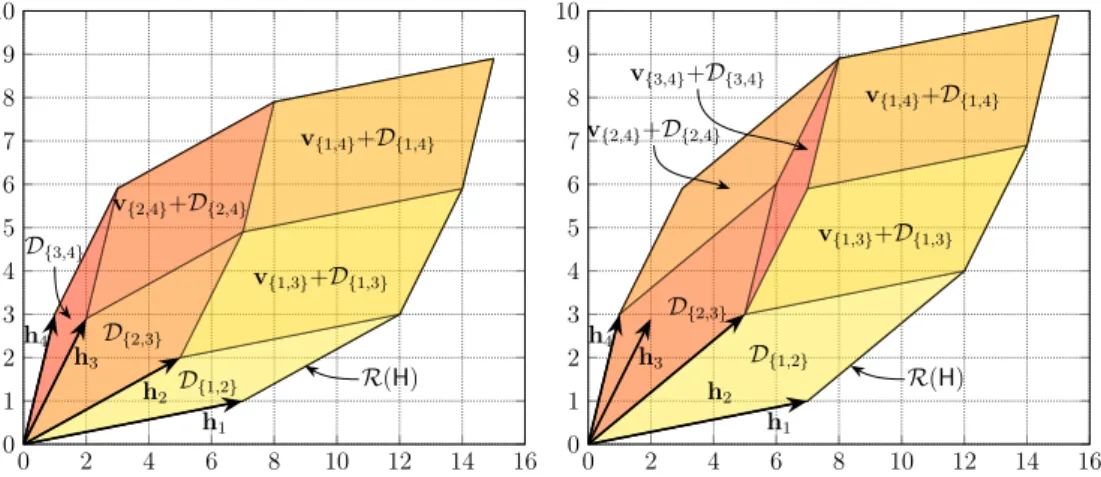
Figure 3.2 shows the partition of R(H) into the union (3.26) for two 2 ⇥ 4 ex-amples. Figure 3.3 shows the union for a 2 ⇥ 3 example when there exist 2 column vectors in the channel matrix that are linearly dependent.

0 2 4 6 8 10 12 14 16 0 1 2 3 4 5 6 7 8 9 10 h1 h2 h3 h4 D{1,2} D{2,3} D{3,4} v{1,3}+D{1,3} v{2,4}+D{2,4} v{1,4}+D{1,4} R(H) 0 2 4 6 8 10 12 14 16 0 1 2 3 4 5 6 7 8 9 10 h1 h2 h3 h4 D{1,2} D{2,3} v{3,4}+D{3,4} v{1,3}+D{1,3} v{2,4}+D{2,4} v{1,4}+D{1,4} R(H)

Figure 3.2: Partition of R(H) into the union (3.26) for two 2 ⇥ 4 MIMO examples. The example on the left is for H = [7, 5, 2, 1; 1, 2, 2.9, 3] and the example on the right for H = [7, 5, 2, 1; 1, 3, 2.9, 3].

Remark 7. If Condition (3.22) holds, then the vector x that solves the minimization problem in (3.5) is unique. M Hence the minimum-energy signaling strategy partitions the image space of vec-tors ¯x into nT

nR parallelepipeds, each one spanned by a different subset of nR columns

of the channel matrix. In each parallelepiped, the minimum-energy signaling sets the nT nR inputs corresponding to the columns that were not chosen either to 0 or

to A according to a the rule specified in (3.21) and uses the nR inputs corresponding

3.4. MIMO MINIMUM-ENERGY SIGNALING 17 0 1 2 3 4 5 6 7 8 9 0 1 2 3 4 5 6 h1 h2 h3 Ah2 +D{1,3} D{2,3} R(H)

Figure 3.3: The zonotope R(H) for the 2 ⇥ 3 MIMO channel matrix H = [2.5, 5, 1; 1.2, 2.4, 2]and its minimum-energy decomposition into two parallelograms.

Chapter 4

Maximum-Variance

Signaling

This chapter describes a maximum-variance signaling that maximizes the trace of the covariance matrix of the random image vector ¯X. We characterize several properties of the corresponding optimal input distribution that are useful to obtain the low-SNR capacity slope in Chapters 5 and 6.

4.1 Problem Formulation

As we shall see in Chapters 5 and 6 ahead and in [28], at low SNR the asymptotic capacity is characterized by the maximum trace of the covariance matrix of ¯X = HX, which we denote

K_X¯¯_X , E⇥( ¯X E[ ¯X])( ¯X E[ ¯X])T⇤. (4.1)

In this chapter we discuss properties of an optimal input distribution for X that maximizes this trace. Thus, we are interested in the following maximization problem:

max

PXsatisfying (2.5)tr KX¯¯X (4.2)

where the maximization is over all input distributions PX satisfying the peak- and

average-power constraints given in (2.5).

4.2 MIMO Maximum-Variance Signaling

The following three lemmas show that the optimal input to the optimization problem in (4.2) has certain structures: Lemma 8 shows that it is discrete with all entries taking values in {0, A}; Lemma 9 shows that the possible values of the optimal X form a “path” in [0, A]nT _{starting from the origin; and Lemma 10 shows that, under}

mild assumptions, this optimal X takes at most nR+ 2 values.

The proofs to the lemmas in this section are given in Appendix A.3.

Lemma 8. An optimal input to the maximization problem in (4.2) uses for each component of X only the values 0 and A:

Xi 2 {0, A} with probability 1, i = 1, . . . , nT. (4.3)

Lemma 9. An optimal input to the optimization problem in (4.2) is a PMF P⇤ X

over a set {x⇤

1, x⇤2, . . .} satisfying

x⇤_{k,`</sub>  x⇤k0<sub>,`} for all k < k0, ` = 1, . . . , nT. (4.4)

Furthermore, the first point is x⇤

1 = 0, and

P_X⇤(0) > 0. (4.5) Notice that Lemma 8 and the first part of Lemma 9 have already been proven in [28]. A proof is given in the appendix for completeness.

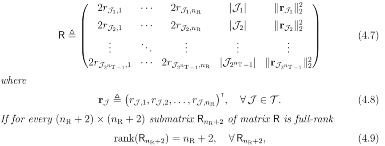
Lemma 10. Define T to be the power set of {1, . . . , nT} without the empty set, and

define for every J 2 T and every i 2 {1, . . . , nR}

r_{J ,i} ,

nT

X

k=1

hi,k {k 2 J }, 8 J 2 T , 8 i 2 {1, . . . , nR}. (4.6)

(Here J describes a certain choice of input antennas that will be set to A, while the remaining antennas will be set to 0.) Number all possible J 2 T from J1 to J2nT 1

and define the matrix

R, 0 B B B B @ 2r_J1,1 · · · 2r_J1,nR |J1| krJ1k22 2r_{J2,1 · · ·} 2r_J2,nR |J2| krJ2k22 .. . . .. ... ... ... 2r_{J2nT 1},1 · · · 2rJ2nT 1,nR |J2nT 1| krJ2nT 1k 2 2 1 C C C C A (4.7) where r_J , r_{J ,1}, r_{J ,2}, . . . , r_{J ,nR} T, _{8 J 2 T .} (4.8) If for every (nR+ 2)⇥ (nR+ 2) submatrix RnR+2 of matrix R is full-rank

rank(RnR+2) = nR+ 2, 8 RnR+2, (4.9)

then the optimal input to the optimization problem in (4.2) is a PMF P⇤

X over a set

{0, x⇤

1, . . . , x⇤nR+1} with nR+ 2 points.

Remark 11. Lemmas 6 and 8 together imply that the optimal ¯X in (4.2) takes value only in the set FCP of corner points of the parallelepipeds {vI +DI}:

FCP, [ I2U ⇢ v_I+X i2I ihi: i 2 {0, A}, 8 i 2 I . (4.10)

Lemmas 9 and 10 further imply that the possible values of this optimal ¯X form a path in FCP, starting from 0, and containing no more than nR+ 2 points. M

Table 4.1 (see next page) illustrates four examples of distributions that maximize the trace of the covariance matrix in some MIMO channels.

4.2. MIMO MAXIMUM-VARIANCE SIGNALING 21

Table 4.1: Maximum variance for different channel coefficients

channel gains ↵ max

PX tr KX¯¯X PX: maxPX tr KX¯¯X H = ✓ 1.3 0.6 1 0.1 2.1 4.5 0.7 0.5 ◆ 1.5 16.3687A2 PX(0, 0, 0, 0) = 0.625, PX(A, A, A, A) = 0.375 H = ✓ 1.3 0.6 1 0.1 2.1 4.5 0.7 0.5 ◆ 0.9 12.957A2 PX(0, 0, 0, 0) = 0.7, PX(A, A, A, 0) = 0.3 H = ✓ 1.3 0.6 1 0.1 2.1 4.5 0.7 0.5 ◆ 0.6 9.9575A2 PX(0, 0, 0, 0) = 0.7438, PX(A, A, 0, 0) = 0.1687, PX(A, A, A, 0) = 0.0875 H = ✓ 1.3 0.6 1 0.1 2.1 4.5 0.7 0.5 ◆ 0.3 6.0142A2 PX(0, 0, 0, 0) = 0.85, PX(A, A, 0, 0) = 0.15 H = 0 @0.9 3.20.5 3.5 1.7 2.51 2.1 0.7 1.1 1.1 1.3 1 A 0.9 23.8405A2 PX(0, 0, 0, 0) = 0.7755, PX(A, A, A, A) = 0.2245 H = 0 @0.9 3.20.5 3.5 1.7 2.51 2.1 0.7 1.1 1.1 1.3 1 A 0.75 20.8950A2 PX(0, 0, 0, 0) = 0.7772, PX(A, A, A, 0) = 0.1413, PX(A, A, A, A) = 0.0815 H = 0 @0.9 3.20.5 3.5 1.7 2.51 2.1 0.7 1.1 1.1 1.3 1 A 0.6 17.7968A2 PX(0, 0, 0, 0) = 0.8, PX(A, A, A, 0) = 0.2

4.3 MISO Maximum-Variance Signaling

When nR = 1, the channel reduces to the MISO channel. Since ¯X in this case is

just a scalar, then the maximum variance of ¯X can be characterized by

Vmax(A, ↵A), max PX¯

Eh _X¯ _{E[ ¯X]} 2i

, (4.11)

where the maximization is over all distributions on ¯X 2 R+

0 satisfying the power

constraints.

The following Lemma 12 characterizes the optimal input to the optimization problem in (4.11) in the MISO channel.

Lemma 12 (Lemma 8, [23]). 1. The maximum variance Vmax(A, ↵A) can be

achieved by restricting P_X¯ to the support set

{0, s1A, s2A, . . . , snTA}. (4.12)

2. The maximum variance Vmax(A, ↵A) satisfies

Vmax(A, ↵A) = A2 (4.13)

where , max q1,..., q_nT 0 : P_nT k=1qk1 P_nT k=1k·qk↵ (_nT X k=1 s2_kqk ✓_XnT k=1 skqk ◆2) . (4.14)

3. The optimal solution q⇤ _{= (q}⇤

1, . . . , qn⇤T) in (4.14) satisfies

PnT

k=1qk < 1 with

strict inequality and PnT

k=1k· qk = ↵ with equality. Furthermore, whenever

rank 0 B B B B B @ 1 _s11 s1 1 2 s2 s2 .. . ... ... 1 nT s_nT snT 1 C C C C C A = 3, (4.15)

the solution q⇤ _{to (4.14) has at most two nonzero elements, i.e., under}

con-dition (4.15), the maximum variance Vmax is achieved by an ¯X⇤ with positive

probability masses at 0 and at most two points from the set {s1A, . . . , snTA}.

See Table 4.2 for a few examples on numerical solution to the maximization problem in (4.14).

For many examples, the optimizing q⇤ _{has only a single positive entry, and thus}

V_max is achieved by an ¯X⇤ that has only two point masses (one of them at 0). Table 4.1 presents some examples of maximum variances Vmax and the probability

4.3. MISO MAXIMUM-VARIANCE SIGNALING 23

Table 4.2: Maximum Variance for Different Channel Coefficients

channel gains ↵ Vmax Q_X¯ achieving V_max

h = (3, 2.2, 0.1) 0.9 6.6924A2 Q_X¯(0) = 0.55, Q_X¯(s2A) = 0.45

h = (3, 2.2, 1.1) 0.7 7.1001A2 Q_X¯(0) = 0.7667, Q_X¯(s3A) = 0.2333

h = (3, 1.5, 0.3) 0.95 5.1158A2 Q_X¯(0) = 0.5907, Q_X¯(s2A) = 0.2780,

Chapter 5

MISO Channel Capacity

Analysis

This chapter presents a new improved upper bound for the SISO channel and new lower and upper bounds for the MISO channel. Many results in this chapter are from [23], and included for completeness; Theorems 14 and 16 are the main new results of this thesis.

5.1 Equivalent Capacity Expression

In this section we first express the channel capacity in terms of ¯X. From Lemma 2 in Chapter 3, we define the random variable U over the alphabet {1, . . . , nT} to

indicate in which interval ¯X lies: ¯

X 2 [Ask 1, Ask) =) U = k, (5.1)

and U = nT if ¯X = AsnT. Let p = (p1, . . . , pnT)denote the probability vector of U:

pk , Pr[U = k], k 2 {1, . . . , nT}. (5.2)

The expression of the channel capacity for the MISO case can then be simplified in the following lemma. The proof can be found in [23].

Lemma 13 (Proposition 3, [23]). The MISO capacity satisfies Ch(A, ↵A) = max

P_X¯

I( ¯X; Y ), (5.3) where the maximization is over all laws on ¯X _{2 R}+₀ satisfying

Pr⇥ ¯X > snTA ⇤ = 0 (5.4a) and nT X k=1 pk ✓ E[ ¯X_{|U = k]} Ask 1 hk + (k 1)A ◆  ↵A. (5.4b) 25

5.2 Capacity Results

5.2.1 A Duality-Based Upper Bound for the SISO Channel

Consider first the SISO channel, where nT = 1 and h1 = 1. So here, the

average-power constraint is active when ↵  1

2. We have the following upper bound:

Theorem 14 (Upper Bound on SISO Capacity). For any µ > 0, the SISO capacity C1(A, ↵A) under peak-power constraint A and average-power constraint

↵A is upper-bounded as: C1(A, ↵A)  log

✓ 1 + pA 2⇡e 1 e µ µ ◆ +p1 2⇡ µ A ⇣ 1 e A22 ⌘ + µ↵ ✓ 1 2_Q ✓ A 2 ◆◆ , (5.5) where Q(·) denotes the Q-function associated with the standard normal distribution.

Proof: See Appendix A.4.1.

5.2.2 A Duality-Based Upper Bound for the MISO Channel

In the following we present an analytic upper bound and compare it to numerical lower bounds. As we will see, the upper bound is asymptotically tight at high-SNR, and can improve on previous bounds in the regime of moderate SNR.

This upper bound is based on Theorem 5.5 and the following Proposition 15: Proposition 15 (Sec. 6, Eq. (88), [23]). Let X⇤ _{be a capacity-achieving input}

distribution for the MISO channel with gain vector h. Define for all k 2 {1, . . . , nT}:

p⇤_k, PrX⇤[U = k], (5.6a)

↵⇤_k, EX⇤

 ¯_{X sk 1A} hkA

U = k . (5.6b) The capacity of the MISO channel is upper-bounded as

Ch(A, ↵A) H(p⇤) + nT

X

k=1

p⇤_kC1(hkA, ↵k⇤hkA), (5.7)

and it holds that

nT

X

k=1

p⇤_k ↵⇤_k+ (k 1)  ↵. (5.8) We can now state our new upper bound on the MISO capacity.

Theorem 16. The MISO capacity is upper-bounded as:

Ch(A, ↵A)  sup p inf µ>0 ( H(p) + nT X k=1 pklog ✓ 1 + pAhk 2⇡e · 1 e µ µ ◆ + pµ 2⇡A nT X k=1 pk hk ✓ 1 e A2h22k ◆ + µ ↵ nT X k=1 pk(k 1) !) (5.9)

5.3. ASYMPTOTIC CAPACITY AT LOW SNR 27

where the supremum is over vectors p = (p1, . . . , pnT) satisfying nT

X

k=1

pk(k 1) ↵. (5.10)

Proof: Combine Proposition 15 and Theorem 14, and use the bound 1 2Q A

2 < 1.

5.3 Asymptotic Capacity at low SNR

Proposition 17. The MISO capacity is upper-bounded as

Ch(A, ↵A) 

1

2log(1 + Vmax(A, ↵A)). (5.11) Proof: Since ¯X and Z are independent, we know that the variance of Y cannot exceed Vmax(A, ↵A) + 1, and therefore

h(Y ) 1

2log 2⇡e(Vmax(A, ↵A) + 1). (5.12) The bound follows by subtracting h(Z) = 1

2log 2⇡e from the above.

In fact, the asymptotic capacity slope at low SNR is only determined by two parameters A and Vmax(A, ↵A). It is shown that

Theorem 18 (Proposition 12, [23]). The low-SNR asymptotic capacity slope is

lim A#0 Ch(A, ↵A) A2 = 2, (5.13) where is defined in (4.14).

5.4 Numerical Results

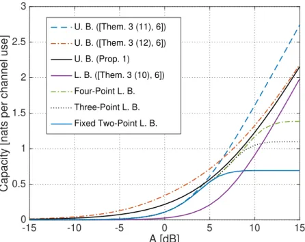
Example 19. Consider a SISO channel with ↵ = 0.4, the numerical results are shown in Figure 5.1. We compare the upper bound (5.5) with the lower and upper bounds in [23]. We also plot numerical lower bound with two, three, and four probability mass points. At low- and moderate-SNR regime, these numerical lower bounds are very close to the new upper bound. This indicates that it gives a good approximation to the capacity and dominates other existing upper bounds in the

moderate-SNR regime. ⌃

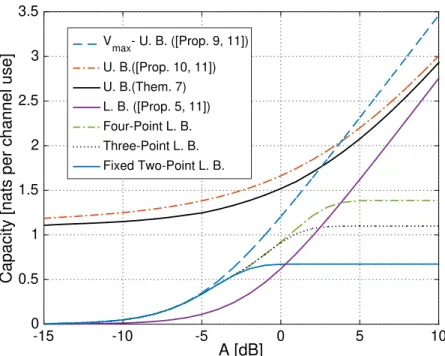
Example 20. Consider the 3-LED MISO channel with gains h = (3, 2, 1.5). The asymptotic low-SNR capacity slope is /2 = 5.07 and is attained by choosing ¯X equal to 0 with probability q0 = 0.6 and equal to s3A with probability q3 = 0.4.

Figure 5.2 shows lower and upper bounds on the channel capacity at different SNR values. The blue lower bound is obtained by numerically evaluating I( ¯X; Y ) for

-15 -10 -5 0 5 10 15 A [dB] 0 0.5 1 1.5 2 2.5 3

Capacity [nats per channel use]

U. B. ([Them. 3 (11), 6]) U. B. ([Them. 3 (12), 6]) U. B. (Prop. 1) L. B. ([Them. 3 (10), 6]) Four-Point L. B. Three-Point L. B. Fixed Two-Point L. B.

Figure 5.1: Bounds on capacity of SISO channel with ↵ = 0.4.

the choice of ¯X that achieves the asymptotic low-SNR capacity. The magenta lower bound follows by numerically optimizing I( ¯X; Y )over all choices of ¯Xthat have pos-itive probability on ¯X = 0 and on at most two point masses from {s1A, . . . , snTA}.

In the low-SNR regime, these numerical lower bounds improve over the previous analytic lower bounds in [23] and are very close to the maximum-variance upper bound in [23, Prop. 9]. The gap between the best upper and lower bounds is larger in the moderate SNR regime. In this regime, the best upper bound (see the black line) is given in Theorem 16. ⌃

5.4. NUMERICAL RESULTS 29 -15 -10 -5 0 5 10 A [dB] 0 0.5 1 1.5 2 2.5 3 3.5

Capacity [nats per channel use]

V max- U. B. ([Prop. 9, 11]) U. B.([Prop. 10, 11]) U. B.(Them. 7) L. B. ([Prop. 5, 11]) Four-Point L. B. Three-Point L. B. Fixed Two-Point L. B.

Figure 5.2: Bounds on capacity of MISO channel with gains h = (3, 2, 1.5) and average-to-peak power ratio ↵ = 1.2.

Chapter 6

MIMO Channel Capacity

Analysis

In this chapter we present new upper and lower bounds on the capacity of the general MIMO channels. As byproducts, we also characterize the asymptotic capac-ity at low and high SNR. The results in this chapter are based on the results in [52], [53].

6.1 Equivalent Capacity Expression

We state an alternative expression for the capacity CH(A, ↵A) in terms of ¯Xinstead

of X. To that goal we define for each index set I 2 U s_I , X

j2Ic

g_I,j, _{I 2 U,} (6.1)

which indicates the number of components of the input vector set to A in order to induce vI.

Remark 21. It follows directly from Lemma 6 that

0_{ sI  n}T nR. (6.2)

M Proposition 22. The capacity CH(A, ↵A) defined in (2.10) is given by

CH(A, ↵A) = max PX¯

I( ¯X; Y) (6.3) where the maximization is over all distributions P_X¯ over R(H) subject to the power

constraint: EU h AsU+ HU1 E[ ¯X|U] vU ₁ i  ↵A, (6.4) 31

where U is a random variable over U such that1

U = _{I =)} X¯ _{2 (vI} +_DI) . (6.5) Proof: Notice that we have a Markov chain X( ¯X ( Y, and that ¯X is a function of X. Therefore, I( ¯X; Y) = I(X; Y). Moreover, by Lemma 6, the range of ¯X in R(H) can be decomposed into the shifted parallelepipeds {vI +DI}I2U.

Again by Lemma 6, for any image point ¯x in vI+DI, the minimum energy required

to induce ¯x is

As_I+ H_I1(¯x v_I) ₁. (6.6) Without loss in optimality, we restrict ourselves to input vectors x that achieve some ¯

x with minimum energy. Then, by the law of total expectation, the average power can be rewritten as E⇥kXk1 ⇤ =X I2U p_IE⇥kXk1 U =I ⇤ (6.7) =X I2U pIE h AsI + H_I1( ¯X vI) ₁ U = I i (6.8) =X I2U p_I⇣As_I+ H_I1 E[ ¯X_{|U = I]} v_{I 1}⌘ (6.9) =EU h AsU + HU1 E[ ¯X|U] vU ₁ i . (6.10)

Remark 23. The term inside the expectation on the left-hand side (LHS) of (6.4) can be seen as a cost function for ¯X, where the cost is linear within each of the parallelepipeds {DI+vI}I2U (but not linear on the entire R(H)). At very high SNR,

the receiver can obtain an almost perfect guess of U. As a result, our channel can be seen as a set of almost parallel channels in the sense of [54, Exercise 7.28]. Each one of the parallel channels is an amplitude-constrained nR ⇥ nR MIMO channel,

with a linear power constraint. This observation will help us obtain upper and lower bounds on capacity that are tight in the high-SNR limit. Specifically, for an upper bound, we reveal U to the receiver and then apply previous results on full-rank nR ⇥ nR MIMO channels [24]. For a lower bound, we choose the inputs in such a

way that, on each parallelepiped DI + vI, the vector ¯X has the high-SNR-optimal

distribution for the corresponding nR⇥ nR channel. M

6.2 Capacity Results

1_{The choice of U that satisfies (6.5) is not unique, but U under different choices are equal with} probability 1.

6.2. CAPACITY RESULTS 33

and let q be a probability vector on U with entries q_I , |det HI| VH , I 2 U. (6.12) Further, define ↵th , nR 2 + X I2U s_Iq_I, (6.13)

where {sI} are defined in (6.1). Notice that ↵thdetermines the threshold value for ↵

above which ¯X can be made uniform over R(H). In fact, combining the minimum-energy signaling in Lemma 6 with a uniform distribution for ¯X over R(H), the expected input power is

E[kXk1] = X I2U Pr[U =_{I] · E[kXk}1|U = I] (6.14) =X I2U q_I ✓ As_I+ nRA 2 ◆ (6.15) = ↵thA (6.16)

where the random variable U indicates the parallelepiped containing ¯X; see (6.5). Equality (6.15) holds because, when ¯X is uniform over R(H), Pr[U = I] = q_I, and because, conditional on U = I, using the minimum-energy signaling scheme, the input vector X is uniform over vI+DI.

Remark 24. Note that

↵th  nT

2 , (6.17)

as can be argued as follows. Let X be an input that achieves a uniform ¯X with minimum energy. According to (6.16) it consumes an input power ↵thA. Define X0

as

X_i0 , A Xi, i = 1, . . . , nT. (6.18)

It must consume input power (nT ↵th)A. Note that X0 also induces a uniform ¯X

because the zonotope R(H) is point-symmetric. Since X consumes minimum energy, we know

E[kXk1] E[kX0k1], (6.19)

i.e.,

↵thA (nT ↵th)A, (6.20)

6.2.1 EPI Lower Bounds

The proofs to the theorems in this section can be found in Appendix A.5.1. Theorem 25. If ↵ ↵th, then CH(A, ↵A) 1 2log ✓ 1 + A 2nR_V2 H (2⇡e)nR ◆ . (6.21) Theorem 26. If ↵ < ↵th, then CH(A, ↵A) 1 2log ✓ 1 + A 2nR_V2 H (2⇡e)nR e 2⌫ ◆ (6.22) with ⌫ , sup 2(max{0,nR₂ +↵ ↵th},min{nR₂ ,↵}) ⇢ nR ✓ 1 log µ 1 e µ µ e µ 1 e µ ◆ inf p D(pkq) , (6.23) where µ is the unique solution to the following equation:

1 µ

e µ

1 e µ = _n

R, (6.24)

and where the infimum is over all probability vectors p on U such that X

I2U

p_Is_I = ↵ (6.25)

with {sI} defined in (6.1).

The two lower bounds in Theorems 25 and 26 are derived by applying the EPI, and by maximizing the differential entropy h( ¯X) under constraints (6.4). When ↵ ↵th, choosing ¯X to be uniformly distributed on R(H) satisfies (6.4), hence

we can achieve h( ¯X) = log VH. When ↵ < ↵th, the uniform distribution is no

longer an admissible distribution for ¯X. In this case, we first select a PMF over the events { ¯X 2 (vI +DI)}I2U, and, given ¯X 2 vI +DI, we choose the inputs

{Xi: i2 I} according to a truncated exponential distribution rotated by the matrix

H_I. Interestingly, it is optimal to choose the truncated exponential distributions for all sets I 2 U to have the same parameter µ. This parameter is determined by the power _nR allocated to the nR signaling inputs {Xi: i2 I}.

6.2.2 Duality-Based Upper Bounds

The proofs to the theorems in this section can be found in Appendix A.5.2.

The first upper bound is based on an analysis of the channel with peak-power constraint only, i.e., the average-power constraint (2.5b) is ignored.